Probing dark gauge boson with observations from neutron stars
Abstract
We present an investigation on the production of light dark gauge bosons by the nucleon bremsstrahlung processes in the core of neutron stars. The dark vector is assumed to be a gauge boson with a mass much below keV. We calculate the emission rate of the dark vector produced by the nucleon bremsstrahlung in the degenerate nuclear matter. In addition, we take into account the photon-dark vector conversion for the photon luminosity observed at infinity. Combining with the observation of J1856 surface luminosity, we find that a recently discovered excess of J1856 hard x-ray emission in the 2–8 keV energy range by XMM-Newton and Chandra x-ray telescopes could be consistently explained by a dark vector with gauge coupling , mixing angle , and mass eV. We also show that the mixing angle for and the gauge coupling for have been excluded at 95% confidence level by the J1856 surface luminosity observation. Our best-fit dark vector model satisfies the current limits on hard x-ray intensities from the Swift and INTEGRAL hard x-ray surveys. Future hard x-ray experiments such as NuSTAR may give a further test on our model.
I Introduction
One of the significant puzzles in particle physics that demand new theory beyond the Standard Model (SM) is the nature of dark matter (DM), whose existence has been confirmed from various cosmological and astrophysical observations Planck2016AA . The most popular class of DM candidates is the weakly interacting massive particles (WIMPs) Lee1977PRL ; Hut1977PLB with a mass at around the electroweak scale and a coupling strength similar to the weak coupling. However, the WIMP hypothesis has suffered stringent constraints due to the null results from both direct XENON1T2018 and indirect Ackermann2015PRL DM detection experiments. As an alternative candidate of DM, a hidden sector consisting of very low-mass particles has drawn more attention in recent years. One of the simplest extensions of the SM is to include an additional gauge group Holdom1986PLB ; Chiang2020PRD , which can naturally arise from the breaking of grand unified theory (GUT) groups Dienes1997NPB ; Ibe2019JHEP or the string theory Dienes1997NPB ; Lukas2000JHEP ; Blumenhagen2005JHEP ; Abel2008JHEP ; Burgess2008JHEP ; Goodsell2009JHEP ; Burrage2009JCAP ; Cicoli2011JHEP . The gauge boson associated with the new group, dubbed the dark photon (which mixes with the SM photon), may play the role of a mediator between the SM and dark sectors or as a dark matter candidate Fabbrichesi2020 .
Supernovae serve as a powerful factory for the emission of dark photons with masses MeV Bjorken1009PRD ; Dent2012 ; Kazanas2014NPB ; Rrapaj2016PRC ; Chang2017JHEP ; Hardy2017JHEP ; DeRocco2019JHEP ; Hong2020 . With a sufficiently weak interaction, dark photons generated within the core of a supernova can escape the progenitor star before their decays, and will contribute to the stellar energy transport. The supernova cooling would be accelerated if the dark photons could transport energy out of the core more efficiently than the standard supernovae cooling via the emission of neutrinos. The bounds on dark photons by using the measurements of SN 1987a have recently been updated in Refs. Chang2017JHEP ; Hardy2017JHEP ; DeRocco2019JHEP , with the consideration of plasma effects for the production of dark photons. The Sun, horizontal branch (HB) stars, and red giants, on the other hand, can serve as important laboratories for dark photons in the mass range of keV. For instance, Refs. An2013PLB ; An2013PRL show that the measured luminosity of the Sun, W, has constrained the dark photon parameter space to the range of An2013PRL .
In this work, we will focus on the production of dark gauge bosons in the core of neutron stars (NSs), which are the remnants of the supernova explosion and have long been recognized as excellent laboratories to search for axionlike particles Iwamoto1984PRL ; Morris1986PRD ; Brinkmann1988PRD ; Iwamoto2001PRD ; Lai2006PRD ; Fortin2018JHEP ; Sedrakian2016PRD ; Sedrakian2019PRD ; Carenza2019JCAP ; Harris2020JCAP ; Buschmann2021PRL ; Leinson2019JCAP ; Leinson2021JCAP ; Fortin2021 . The core of a NS is composed of highly degenerate nuclear matter that has an average density of , which corresponds to an average distance of fm between nucleons. Dark gauge bosons can be produced through bremsstrahlung of proton and neutron scattering in the NS cores. In the previous literature Chang2017JHEP ; Hardy2017JHEP ; DeRocco2019JHEP , the nondegenerate limit has been assumed to obtain the dark vector emission rate as well as the constraints on the dark vector from the supernova, where the plasma is thought to be diluted and nonrelativistic. However, the nuclear matter in the NS core is in fact highly compressed, and therefore, in this work, we will present the calculation of the production of the dark vector in the NS core in the degenerate limit.
The in-medium effects can lead to a suppression on the dark vector production rate if the dark vector which couples coherently to the charged SM plasma has a mass much below the stellar plasma frequency Chang2017JHEP ; Hardy2017JHEP . In additional to the electromagnetic (EM) current through mixing, the new gauge boson could couple to the current in the well-known theory of extension of the SM Davidson1979PRD ; Marshak1980PLB ; Mohapatra1980PRL ; Davidson1987PRL ; Montero2009PLB ; Ma2014PLB . For such a theory, the new vector boson will dominantly be produced by the neutron bremsstrahlung in the NS core. This is because, for one thing, neutron is the dominant component of the NS, and for another, the vector boson emitted by the neutron in the initial or final state is not suppressed by the plasma effects. In this work, we will assume that the dark gauge boson is the gauge boson with a mass much below keV, the core temperature of the NS, and the gauge coupling is sufficiently small.
Recently, a significant excess of hard x-ray emission in the keV energy range was found by analyzing the data from the XMM-Newton and Chandra x-ray telescopes Dessert2020APJ observing on the nearby magnificent seven (M7) x-ray dim isolated NSs. The excess was interpreted as the emission of axions by the NS in Ref. Buschmann2021PRL and was found to be consistent with the current constraints. In this work, we explore the interpretation of a dark vector scenario for the J1856 hard x-ray excess. We calculate the dark vector emission rate in the NS core and simulate the evolution of the NS based on the modified NSCool code Page2016 , including the dark vector emissivity. Due to the strong magnetic field of the magnetospheres surrounding the NSs, the dark vectors produced in the NS cores may convert into x-rays when they propagate outwards Fortin2019JCAP . We present an analytical formula of the dark vector-photon conversion probability for dark vector with mass , where and are the surface temperature and radius of the NS, respectively. We also calculate the surface luminosity observed at infinity by taking into account the photon-dark vector conversion. Based on the Bayesian inference, the analysis of J1856 hard x-ray data, as well as surface luminosity observation are carried out by the UltraNest package Buchner2021 . We find that the dark vector scenario is favored by the hard x-ray excess, and we also derive 95% upper limits on the model parameters from the data.
The structure of this paper is arranged as follows. Section II defines the dark gauge boson model considered in this work, and sets up the required notations. In Sec. III, we calculate the production of dark vectors from nucleon bremsstrahlung, including the squared matrix element and emission rate. In Sec. IV, we briefly review the neutrino and photon luminosities for the NS cooling. We also calculate the photon surface luminosity observed at infinity that includes photon-dark vector conversion. In Sec. V, we describe the NS simulation based on the modified NSCool code in detail. In Sec. VI, we compute the hard x-ray spectrum from the dark vector-photon conversions. The statistical analysis of data based on the Bayesian inference is carried out in Sec. VII, and the 95% upper limits on the dark vector model are derived in Sec. VIII. Finally in Sec. IX, we summarize our findings. The plasma effects on dark vector’s production are discussed in Appendix A. The dark vector-photon conversion probability is derived in Appendix B. In Appendix C, we show the analytical results for the dark vector-photon conversion probability. The detailed calculations of the dark vector emission rate are given in Appendix D. Discussions on the one-pion approximation are presented in Appendix E.
II The model
We are interested in the extension of the SM with an additional gauge symmetry, having a new gauge boson called the dark vector. The relevant effective Lagrangian at low scales is written as
| (1) |
where we assume the dark vector has a Stueckelberg mass , and are, respectively, the field strengths of the SM photon and dark gauge boson, and represents the mixing angle between the SM photon and dark vector. The parameter denotes the coupling between and the current , which in this work is assumed to be the SM current arising from a symmetry, as widely investigated in the literature Davidson1979PRD ; Marshak1980PLB ; Mohapatra1980PRL ; Davidson1987PRL ; Montero2009PLB ; Ma2014PLB . The kinetic terms of gauge boson in the Eq. (1) can be diagonalized by rotating the gauge fields as
| (2) |
where and are the so-called interaction eigenstates and mass (propagating) eigenstates, respectively. For a massive dark vector, the rotation angle is locked at zero Fabbrichesi2020 . We see that the mixing leads to the interactions between the dark vector and the SM charged particles, such as electron, proton and charged pions, with a coupling strength . Furthermore, due to the mixing, the dark vector can convert to a photon during their propagation.
In the plasma of supernovae, the visible photon develops a nonzero mass that is determined by the plasma frequency , where the sum goes over the charged particles with a number density and a Fermi energy . The nonzero plasma mass of the photon can lead to inequivalent effective couplings to the charged particles in the plasma and in the vacuum (the Lagrangian parameter). The effective coupling between the SM fermions and in the medium is given by Hong2020
| (3) |
where denotes the SM fermions with an electric charge and a dark gauge quantum number in units of and , respectively. The proton and neutron have the electric charges and , and the dark gauge quantum numbers . The EM and dark gauge quantum numbers for the electron are . The visible photon mass is encoded in the polarization tensor given in Appendix A.
From Eq. (3), the effective couplings of electron, proton, and neutron to in a dense medium (i.e., with ) are explicitly given by
| (4) |
We observe that the dark vector couplings to the electrically charged fermions are suppressed by both the mixing term in the Lagrangian and medium-induced effects, while the interaction of to the neutrons is not suppressed by the plasma effects. As a result, there exists a suppression from the plasma effect in the emission of dark vectors from the electron and the proton currents. On the other hand, the production of dark vectors via the neutron current does not have such a suppression, and the emission rate from neutrons in the medium can be approximated by that in the vacuum.
For a NS of interest here, because of the large number of neutrons in a NS core, the dark vectors can be copiously produced via the bremsstrahlung process involving the neutron current. Furthermore, since we are concerned with the case of low dark vector masses, the contributions from the electron and proton bremsstrahlung processes in the crust can and will be neglected. Note that the nucleon superfluidity in the NS core is still under debate. At temperatures below the critical temperature of Cooper pair formation, the nucleon bremsstrahlung rate may be suppressed by nucleon superfluidity. However, recent studies Potekhin2020MNRAS on NS cooling indicate that neutron superfluidity in the middle-aged NS core is weak and the critical temperatures are possibly too low to be relevant for our analyses. Thus, following Ref. Buschmann2021PRL the nucleon superfluidity effect will be ignored in our work.
There exists oscillations between dark vector and photon due to the mixing term in our model. In the presence of an inhomogeneous external field, the approximation for the dark vector-photon conversion probability in the weak-mixing limit is given by
| (5) |
The integral starts from the stellar surface since the x-ray photons produced inside the NS would be absorbed. The parameters and detailed calculations for Eq. (5) are presented in Appendix B. For , we find an analytical formula of Eq. (5), which can be found in Appendix C. We will see that the NS is an excellent test bed for the dark vector hypothesis since the conversion probability can be largely enhanced under a strong magnetic field. For the approximation to make sense, cannot take the vanishing limit and the numerical value for should be sufficiently small to satisfy the weak-mixing condition.
A few remarks are in order. The traditional model is gauge-anomaly free if right-handed neutrinos are introduced. While anomaly free at higher energies, the effective Lagrangian (1) is anomalous due to the mixing term at low energies. And it is the phenomenology of this low-energy effective Lagrangian (1) that we want to discuss in this work. We also note that the constraints on that we obtain from NS cooling in this work do not depend on the mixing term and can be applied to the traditional model.
III Dark vector production
In this section, we calculate the emission rate of dark vectors from the neutron bremsstrahlung in the NS core. Supplements for the calculations are given in Appendix D.
III.1 Dark vector emission rate
The dark vector energy emission rate per unit volume for the process () in a strongly degenerate nuclear matter is given by Brinkmann1988PRD ; Harris2020JCAP
| (6) | ||||
where the symmetry factor for the identical particles in the initial and final states and for mixed processes, the squared matrix element sums over initial and final spins, is the energy of emitted dark vector, is the momentum associated with the nucleon (), and is the momentum of the dark vector. In the presence of a nuclear mean field , the energy dispersion relation of the nucleon is modified to be
| (7) |
where is the effective nuclear mass and is the effective energy. Note that the nuclear energies that enter the energy -function and the denominator on the right-hand side of Eq.(6) are the effective energies Harris2020JCAP . The fermion phase-space distribution function is given by
| (8) |
where is the nuclear chemical potential of . With Eq. (7) we have , where . The occupation numbers and the Pauli blocking factors are for the incoming and outgoing nucleons. The dark vector are assumed to escape freely so that a Bose stimulation factor as well as its absorption are neglected.
In the nonrelativistic (NR) limit, the nucleon effective mass is much larger than all other energy scales such as the temperature or Fermi energies, so that the energy taken by the nucleon is , where is the nuclear kinetic energy. In a bremsstrahlung process, the radiation typically carries the momentum and, therefore, the outgoing nucleons carry essentially all of the momentum and the radiation momentum can be neglected. With these approximations, we show in the next section the scattering matrix element of the nucleon bremsstrahlung, and in Appendix D we calculate the emission rate (6) in the degenerate limit.
III.2 Squared matrix element
As shown above, the effective couplings of to electron and proton in the medium are suppressed in the limit of light . The emission of dark vector from the neutron-neutron bremsstrahlung is the primary production mechanism in the inner core of a NS. The nucleon-nucleon interaction in the nucleon-nucleon bremsstrahlung was treated by the one-pion-exchange (OPE) approximation in Ref. Friman1979APJ and was used in the calculation of the axion emission rate from the nucleon-nucleon bremsstrahlung Brinkmann1988PRD . For our present work, it is sufficiently reliable to calculate the dark vector emission rate using the OPE approximation (see also Ref. Dent2012 ). Conservatively, we also include a factor of Beznogov2018PRC in the emission rate to account for the overestimation in the OPE approximation at lower temperatures Hanhart2001PLB . Additional remarks on the OPE approximation are provided in Appendix E.
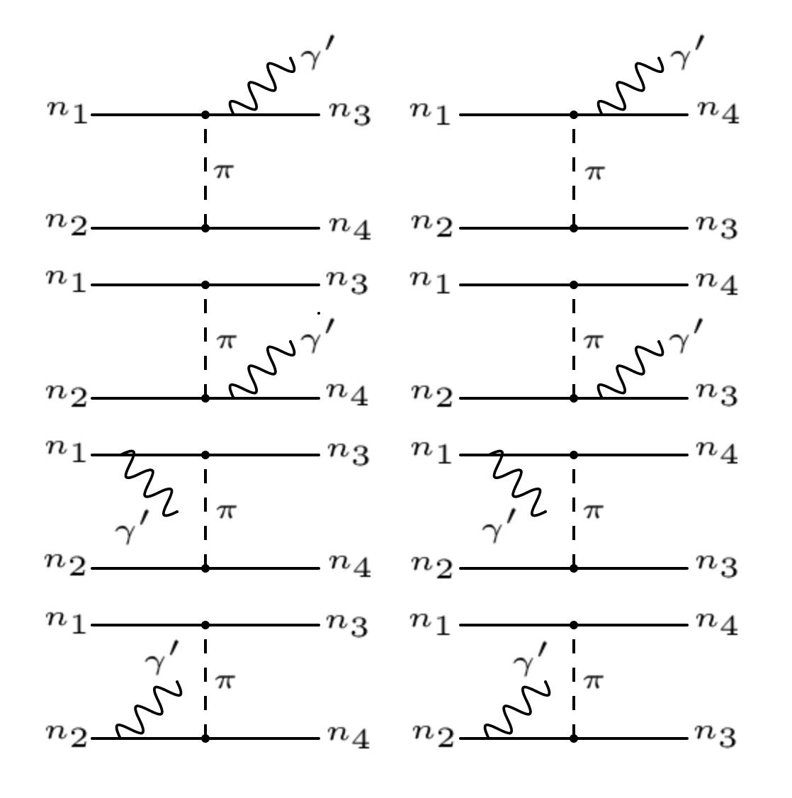
We show the Feynman diagrams for the process (where ) in Fig. 1. The dark radiation is induced by the neutron in the initial and final states in the scattering via the exchange of a neutral pion. The squared matrix element is given by Dent2012
| (9) |
where is the pion mass, the momenta , , with being the four-momenta associated with (), and and . In the NR limit, the nucleon mass is much larger than the temperature, the dark vector mass, and the transferred momenta, i.e., . Furthermore, the four-momenta transferred among the nucleons are much larger than the momentum carried by the dark vector, i.e., . For the model considered in this work, the coefficients are given by
| (10) |
where and is the pion-neutron coupling, the parameter is the coupling between and neutron. We see that only the coefficient is nonzero.
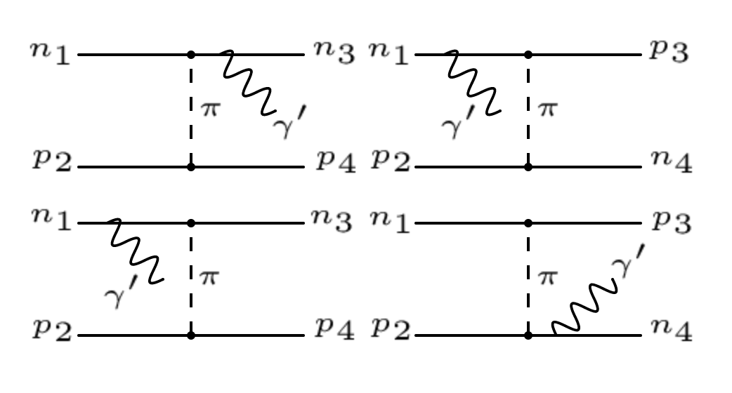
The Feynman diagrams for the process are depicted in Fig. 2. The squared matrix element for this process is given by
| (11) |
where , with as required by isospin invariance. Due to the plasma effects, we have neglected the diagrams where the dark vector is emitted from an electron or proton.
III.3 Dark vector luminosity
Given the emission rate, to compute the luminosity of dark vectors from the NS core we need to know the NS equation of state (EOS), which determines the matter distribution in the NS, the chemical potential of the matter, and the profiles of neutron and proton Fermi momenta. In our analysis, we employ the Akmal-Pandharipande-Ravenhall (APR) EOS Akmal1998PRC to model the uniform nuclear matter in the NS core and assume a NS mass of , which corresponds to a NS core radius of km. It is expected that the nucleon bremsstrahlung in the NS core dominates the production of dark vectors. For the weak coupling theory, the mean free path of dark vector in the medium is much larger than the size of the NS. So in the calculation we have neglected the dark vector reabsorption effect.
The differential dark vector luminosity is given by integrating the differential emissivity over the volume of the NS
| (12) |
Integrating the differential luminosity over , we obtain the total dark vector luminosity. With the APR EOS for the NS and a light dark vector with mass keV, the dark vector luminosity from the NS core can be estimated as
| (13) |
where is the core temperature of the NS. The emission of dark vectors can result in NS cooling. Since the standard NS cooling scenario in terms of neutrino and photon emissions fits rather well to the observation of the NSs, the stellar cooling can be used to constrain the dark vector model.
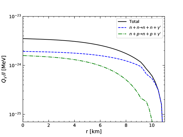
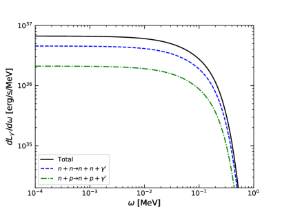
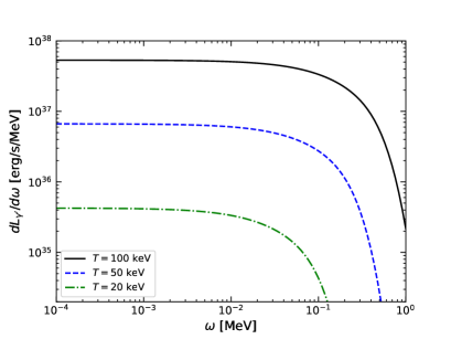
In Fig. 3, we plot the dark vector “energy emission rate” , where is given by Eq. (61), as a function of the NS radius, with eV and . The dashed and dot-dashed curves represent the results for the process and , respectively. As expected, the neutron-neutron bremsstrahlung dominates the emission of dark vectors. The nearly constant emission rate extends to the radius km and decreases sharply when approaching the surface. We show the differential luminosity of dark vectors as a function of the dark vector energy in Fig. 4, again with eV and . As shown in the left plot of Fig. 4, the differential luminosity of dark vectors is nearly a constant for and cuts off at due to the factor in the differential luminosity. In the right plot of the figure, we observe that both the constant regime and the cutoff point of increase with the NS core temperature.
IV Neutrino and photon luminosities
One of the most fascinating stars known in the Universe is the NS, whose birth in supernova explosions is accompanied by the most powerful neutrino outburst. The standard NS cooling scenario based upon the pioneering works Chiu1964PRL ; Bahcall1965PLBa ; Bahcall1965PLBb ; Friman1979APJ ; Maxwell1987APJ includes several neutrino emission processes (see Yakovlev2001PR for a review). The direct Urca cooling process consists of beta decay and electron capture that can induce a huge sink of energy in the NS core. However, a sufficiently small separation between the Fermi levels of protons and neutrons is required to activate this mode, which generally requires a minimum mass of the NS, denoted by , that is significantly larger than the canonical NS mass of Lattimer1991PRL ; Beloborodov2016APJ . For the NS with mass less than , the modified Urca cooling mode can take place everywhere and dominate the NS cooling process. The modified Urca process is similar to the direct Urca, but involves an additional nucleon spectator,
| (14) | |||
| (15) |
The modified Urca by the neutron branch is shown by Eq. (14). Its neutrino emission rate in the NS core is given by Friman1979APJ
| (16) |
where is the NS mass density profile, is the nuclear saturation density, is the NS core temperature, and the suppression factor appears with the onset of superfluidity. Cooper pair cooling could become dominant if the superfluidity occurs. However, as argued above, the critical temperature for the Cooper pair formation is possibly too low to be relevant for this work. We thus do not take the superfluidity into account.
The proton branch, Eq. (15), was first analyzed in Ref. Yakovlev1995AA by using the same formalism as that in Ref Friman1979APJ . The expression for the neutrino emissivity in the proton branch can be approximated by the following rescaling relation Yakovlev2001PR
| (17) |
where and are the effective masses of proton and neutron, respectively, and , , and are the Fermi momenta of electron, proton, and neutron, respectively. Note that for ; otherwise, . As an example, take , we have , i.e., the proton branch is nearly as efficient as the neutron branch. In addition to the Urca processes, the neutrino’s emission processes can also be induced by the bremsstrahlung in nucleon-nucleon collisions, which, however, are subdominant for the NS cooling (a summary of these processes can be found in Figs 11 and 12 of Ref. Yakovlev2001PR ). Summing up all of the processes, the total neutrino emission rate can be estimated as , with a rescaling factor Yakovlev2001PR . With the neutrino emission rate, we can then determine the neutrino luminosity by the integration
| (18) |
where km is the NS core radius. For the APR EOS, the neutrino luminosity is then given by
| (19) |
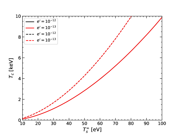
Previous literature has obtained the constraints on new physics models, e.g., the axion coupling, by requiring that the emissivity of the new particle should not exceed that of the neutrino, i.e., Raffelt1996 . Otherwise, the evolution of the NS will be strongly altered by the new physics, which is in conflict with the observations. As shown above, in addition to the NS density profile, the luminosities of dark vector and neutrino strongly depend on the core temperature, which, however cannot be determined by the EOS or by direct measurements. The core temperature may be inferred from the NS surface temperature observations but suffers from large uncertainties Buschmann2021PRL . In Fig. 5, we depict the relation between core temperature and surface temperature at infinity using NSCool code Page2016 (with the default NS model). We observe that the relation is independent of the new gauge coupling (with ). However, as we will show below, the luminosity at infinity cannot be solely determined by the luminosity at NS surface if there are conversions between photon and dark vector during their propagation toward the observer. In this case, there is no direct relation between core temperature and surface temperature at infinity. Furthermore, in the standard NS evolution, the additional heating effects can be neglected for the middle-aged NS, and the evolution of the NS core temperature with the time is expected to follow a power law Beloborodov2016APJ . Such a relation may also break down in new physics if the cooling of the NS is strongly affected by the emissions of new weakly-interacting particles. In this work, we will perform numerical simulations of the NS cooling based on the modified NSCool code that includes additional energy loss via the dark vector emission. In this way, we determine the core temperature and the surface luminosity for the NS with a given age. This will be described in detail below.
In the standard NS cooling model, the emissions of neutrinos and photons lead to the NS cooling. In the early stage, the neutrino emission is the dominant mode for the NS cooling. As the stellar temperature drops, the NS cooling by photon emissions becomes significant since the neutrino luminosity decreases much faster than that of photon. For NSs with age kyr, the photon emission will exceed the neutrino one Raffelt1996 , and thus dominates the NS cooling process.
We now turn to the photon emission of the NS. The NS cooling due to the emission of photons is directly measured by the NS surface photon luminosity, which is given by
| (20) |
where is the Stefan-Boltzmann constant, is stellar radius, and is stellar surface temperature. Without photon-dark vector conversions, the observed surface photon luminosity at infinity is accordingly redshifted as
| (21) |
where is the gravitational potential at the stellar surface, and
| (22) |
where is the gravitational constant, and is the stellar mass.
However, the observed surface photon luminosity will be changed if the photons and dark vectors can convert into each other during their propagation to the Earth. For the NS with age yr that is concerned in this work, we will show that the surface luminosity of the NS will be dominated by the photon emissions. For the parameter space we are interested in, the dark vectors’ luminosity is always a subdominant component and, therefore, their contributions to the observed photon luminosity will be neglected. In this case, the surface photon luminosity observed at infinity is given by
| (23) |
where is the photon-dark vector conversion probability, which will be given in Appendix B. Since the Stefan-Boltzmann law (20) can be obtained by integrating the Planck’s law over , the differential surface luminosity of the photon is given by
| (24) |
We will show in Appendix C that the conversion probability can be written as for dark vector in the mass range eV, with eV. With these, we finally obtain the observed surface photon luminosity at infinity by taking into account the conversion
| (25) |
where . The surface temperature at infinity is then given by
| (26) |
Using these results, we can determine the observed surface luminosity and temperature by including the redshift by the gravitational potential as well as the conversion once we know the values of and at the NS surface.
The validation of Eqs. (25) and (26) should be further clarified. One may be concerned that the approximation of the probability requires . However, we have integrated over in the range of for . It is easy for the reader to confirm that there is nearly no difference between the integration over in the ranges of and , which means that the small values of make negligible contributions to the integration. We thus conclude that Eqs. (25) and (26) are valid for our calculations provided that , with eV.
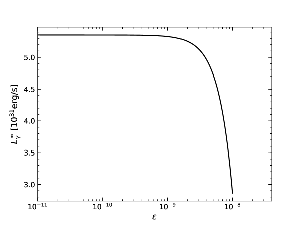
In Fig. 6, we show the variation of the surface luminosity observed at infinity with the mixing angle . We assume the surface luminosity erg/s and temperature eV for the NS. As shown in this figure, the conversion strongly reduces the observed surface luminosity when the mixing angle reaches values of .
V NS cooling simulation
In this work, we employ the NSCool code Page2016 for the numerical simulation of the thermal evolution of the star. The current version of the NSCool code incorporates all the corresponding neutrino cooling reactions, including direct and modified Urca processes, nucleon-nucleon bremsstrahlung, as well as the thermal Cooper pair breaking and formation (PBF). We modify the code to include the emissivity of the dark vector so that it can take part in the NS cooling along with the neutrino emission processes. For the core of the NS, we adopt the APR EOS with a mass (Prof_APR_Cat_1.4.dat). For the crust EOS, we use the default profile implemented by the file Crust_EOS_Cat_HZD-NV.dat.
We focus on the observations from one of the M7 members, RX J1856.5-3754 (J1856 for short), which locates at a distance pc away from us and has an age around yr Kerkwijk2008PAJ ; Walter2010APJ (a summary can be found in Refs. webNScool ; Potekhin2020MNRAS ). Recent studies Potekhin2020MNRAS on NS cooling indicate that the critical temperature is very low and the neutron superfluidity is very weak for the middle-aged NS. We thus turn off the PBF processes in the simulations with NSCool, as is done in Ref. Buschmann2021PRL . We find that the results from the standard NS cooling without including the PBF processes can account for the surface luminosity observations on J1856 quite well. However, the simulation including the PBF processes predicts a much lower surface luminosity than the observation.
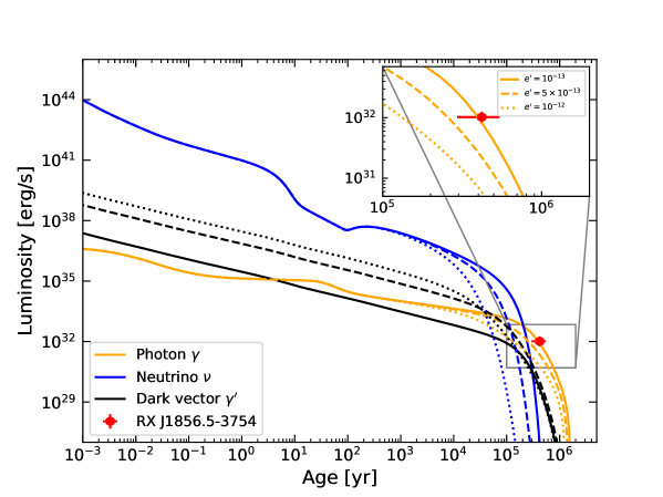
In Fig. 7, we depict the neutrino (blue), dark vector (dark), as well as photon (yellow) surface luminosities as a function of the NS age. In the simulations, we assume , and , and the results are represented by the solid, dashed, and dotted curves, respectively. The blue, dark, and yellow curves represent the neutrino, dark vector, and photon surface luminosities, respectively. The red point represents the observation of the J1856 surface luminosity. It is shown by the simulations that the photon luminosity is the dominant component for J1856. We find that the model with a new gauge coupling predicts the same age-luminosity profile as the standard NS cooling model since in this case the cooling by the dark vector emission is negligible. There is a significant deviation in the photon luminosity from the observation when increases to and, therefore, should be constrained by the observation. We will show the constraints on the model by fitting to the observations below.
VI x-ray from dark vector-photon conversion
Recent analyses of the data from the XMM-Newton and Chandra x-ray telescopes Dessert2020APJ show a significant excess of hard x-ray emissions, in the energy range of keV, from the nearby M7 x-ray dim isolated NSs. In particular, it has been shown in Ref. Dessert2020APJ that the NS J1856 hard x-ray spectrum has a excess, which is the most significant hard x-ray excess among the M7 members. The fact that the hard x-ray excess is observed in some NSs but not others depends on the experimental measurements as well as the NS properties Buschmann2021PRL . Observations by the ROSAT All Sky Survey Haberl2007ASS have shown that all the M7 members have soft spectra that are well described by near-thermal distributions with surface temperatures eV and, therefore, they are expected to produce negligible hard x-ray flux. The explanation of the hard x-ray excess in the context of an axion model has been explored in Ref. Buschmann2021PRL and is found to be consistent with the current constraints. In this work, we explore the interpretation for the excess in the dark vector scenario.
The conversion probability between dark vector and photon is proportional to the square of the magnetic field strength. Observations show that all the M7 NSs have strong magnetic fields with a characteristic dipole magnetic field strength around G. Therefore the NSs provide an excellent place to test the oscillations. Having calculated both the differential luminosity of dark vectors (12) and the dark vector-to-photon conversion probability in Appendix B, the differential flux of hard x-ray photons produced from dark vector-photon conversion is given by
| (27) |
where is the distance between the NS and Earth. The probability depends on the dipole magnetic field orientation . In this work we adopt the -averaged conversion probability as an approximation for our calculations. In the limit of small dark vector mass, eV for energy keV and NS radius km, becomes independent of (see Eq. (56) in Appendix C). Note that in order to compare with the observed hard x-ray spectrum, the differential flux is calculated at energy , where is the observed photon energy. Then the differential flux observed at infinity is given by . Compared with the photon differential luminosity whose maximum value is obtained at energy eV, with a surface temperature eV, the hard x-ray spectrum from conversion has its maximum value at a much higher energy keV, with a core temperature keV (the surface-core temperature relation can be found in Fig. 5). We thus expect the flux from conversion can make contributions to the hard x-ray excess in the energy range keV and at the same time reproduce the correct spectrum shape.
VII Statistical analysis
Our starting point for the statistical analysis of the J1856 data in the context of the dark vector model is the Bayesian inference Bayesian1992 . For the model consisting of a set of parameters , the Bayes theorem is given by
| (28) |
where is the data probability, is the prior probability that indicates the degree of belief one has before observing the data, and is the conditional probability-density function that is a posterior probability representing the change in the degree of belief one can have after giving the measurement data. Note that links the posterior probability to the likelihood of the data, where the likelihood function takes the form of
| (29) |
where
| (30) |
where denotes the experimental value with an uncertainty in the measurement , represents the number of data points, and denotes the predicted value for a given model.
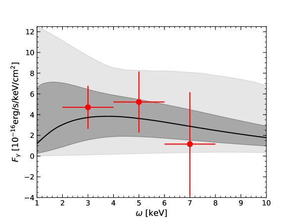
For the dataset, we take into account the J1856 x-ray spectrum observations in keV Dessert2020APJ , Buschmann2021PRL , Ho2007MNRAS ; Mignani2013MNRAS ; Yoneyama2017PASJ , and the distance measurements Kerkwijk2008PAJ ; Walter2010APJ . Noting that inferred from the observations is in a narrow band erg/s, we take erg/s as the central value and assume a Gaussian distribution for the luminosity. The parameter set is , where the distance enters the spectrum function. We fix the mass of dark vector eV to establish the approximation of conversion probability, i.e., Eq. (56). Note that our analysis is independent of as long as , with surface temperature eV.
The performance of the Bayesian statistical analysis is carried out using the UltraNest package Buchner2021 , which implements a nested sampling Monte Carlo technique Skilling2004 . It computes the (log-)likelihood as well as the marginal likelihood (“evidence”) to perform model comparison. Meanwhile, the posterior probability distributions on model parameters are constructed to describe the parameter constraints of the data. We assume a uniform prior distribution for the distance and a log-uniform prior distribution for and . We choose the number of live points to be 20000, and the total number of the samples called in the fitting is 225802.
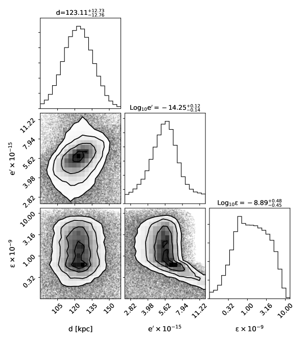
In each running, we simulate the NS cooling based on the modified NSCool code that includes the dark vector emissivity. We then determine the surface luminosity as well as the surface temperature at the age of J1856. We obtain a minimum value (corresponding to the maximum value of the likelihood) of the reduced chi-square in the fitting to the data. On the other hand, when the emissivity of dark vector is turned off in the fitting, we obtain a value of with the NS standard cooling model. We thus conclude that we have made the fitting much better by taking into account the emission of dark vectors. Therefore, the data supports the existing of a dark vector with couplings summarized in Table 1.
| Parameter | Prior range | Best-fit | Mean/ range | Median/ range |
|---|---|---|---|---|
| [kpc] | 122.870 | |||
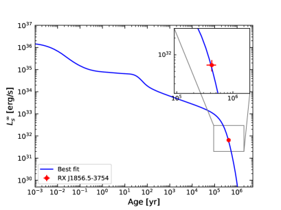
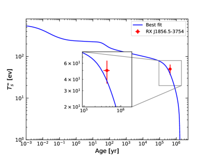
The corner plot in Fig. 8 shows the posterior distributions of the parameters. In Fig. 9, we show the predictions of the model for the J1856 x-ray spectrum. The black curve denotes the prediction of the model with the median values, while the black band represents the confidence interval. Figure 10 depicts the evolution of the surface luminosity and temperature observed at infinity with the NS age. In this plot, we take the parameters to their best-fit values. As indicated in these figures, the x-ray spectrum as well as the luminosity observations can be well interpreted in the dark vector model. We note that all of the PBF processes have been turned off in our simulations. Including these processes would lead to much lower surface luminosities than the observations.
VIII Model constraints
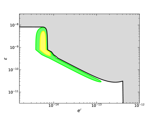
The likelihood ratio test Rolke2005 is used to determine the limit on and the significance of a possible dark vector contribution to the J1856 observations. To do this, we fix and determine the “nuisance parameter” by minimizing the chi-square. Upper limits at the 95% confidence level on are derived by increasing the chi-square from its minimum value of the model until it changes by 2.71, , with denoting the parameter that minimizes the chi-square at fixed . The black curve in Fig. 11 represents the constraints on and the grey region is excluded by the constraint. The green and yellow regions represent the parameter spaces that are favored by the observations at and confidence intervals. The conclusions inferred from this figure are summarized as follows:
-
•
There is an upper limit on the mixing angle , which is independent of the gauge coupling and dark vector mass (as long as eV). This is because the observed surface luminosity would be strongly suppressed by the conversion when , as illustrated in Fig. 6. This constraint can also be applied to the dark photon model.
-
•
There is an upper limit on the gauge coupling , which is independent of the mixing angle and dark vector mass (as long as keV). This is because the surface luminosity would be strongly reduced due to the cooling of the NS by the dark vector emissivity with , as shown in Fig. 7.
-
•
For the gauge coupling in the range of , the x-ray spectrum data dominates the contributions to chi-square. We have shown that the model with parameters around the mean values and can explain the x-ray spectrum excess in the energy band keV. Since the x-ray spectrum from the new physics is proportional to , constraints on become stronger with the increase of .
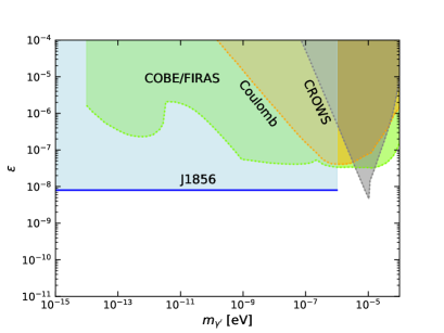
In Fig. 12, we compare our constraints with those limits from cosmological, astrophysical, as well as terrestrial observations. In the left plot of the figure, we summarize the constraints on the mixing angle in the low mass range eV. The oscillation between the ordinary photon and the massive dark photon induces deviations on the black body spectrum in the cosmic microwave background, which has been constrained by the COBE/FIRAS experiment Fixsen1996APJ ; Caputo2020PRL ; Aramburo2020JCAP ; McDermott2020PRD (light-green region). The constraints from detecting modifications of Coulomb force by the new gauge force in atomic and nuclear experiments are depicted by the orange region Jaeckel2010PRD . Using the phenomenon of light shining through a wall for dark photons, the grey region has been bounded by the experiment CROWS Betz2013PRD at CERN. We observe that our constraint (light-blue region) on from J1856 surface luminosity observation is much stronger than the above constraints by about an order of magnitude.
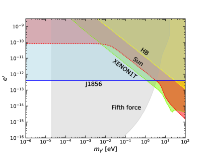
In the right plot of Fig. 12, we summarize the constraints on the gauge coupling . The exchange of light bosons, such as gauge bosons, scalar axions, and dilatons among others generates a Yukawa potential, which is tested by the fifth force experiments Sushkov2011PRL ; Murata2015CQG ; Chen2016PRL . Furthermore, light boson states emitted from the Sun may be probed in the DM direct detection experiments An2020PRD ; XENON1T2020 ; PandaX2021 . We compare our NS cooling constraint from J1856 (blue region) with the constraints given by the Sun (red) Hardy2017JHEP , HB (orange) Hardy2017JHEP , XENON1T (green) An2020PRD , and the current fifth force experiments (light-grey) Sushkov2011PRL ; Murata2015CQG ; Chen2016PRL . We observe that the fifth force experiments give the most stringent constraints for eV. Constraints from J1856 surface luminosity observation are much stronger than those given by the Sun luminosity observations and the DM direct detections, for the dark vector with mass eV. In summary, we conclude that the parameter space with eV, for explaining the hard x-ray excess, remains available when various observation constraints on the dark vector model are taken into account.
| Experiment | Energy band | Intensity limit | Predicted intensity | Reference |
|---|---|---|---|---|
| Swift | Oh2018APJ | |||
| INTEGRAL | Krivonos2019MSAI | |||
| NuSTAR | Buschmann2021PRL | |||
| NuSTAR | Buschmann2021PRL |
In Table 2 we summarize the current limits on hard x-ray intensity for NSs near the galactic plane (J1856, J0806, J0720, and J2143) from the 105-month Swift Burst Alert Telescope all-sky hard x-ray survey Oh2018APJ and the 14-year INTEGRAL galactic plane survey Krivonos2019MSAI . We also adopt the projected sensitivity (provided in the supplementary materials of Ref. Buschmann2021PRL ) at 95% confidence level for a 400 ks NuSTAR observation of J1856 in two energy bands. The third column provides the predicted intensities, assuming the median values of the parameters for the dark vector model. We observe that the predicted intensities are far below the current limits from Swift and INTEGRAL, and future observations on M7 by the NuSTAR experiment may be useful to test the dark vector model.
IX Summary and conclusions
The NS is recognized as one of the most excellent astrophysical laboratories for searching for new light particles that couple weakly to SM particles. In this work, we have presented the emission of light dark vectors from the nucleon bremsstrahlung processes in the core of the NS. The dark vector is assumed to be a gauge boson and to have a mass much below about keV, the core temperature of the NS. The dominant production mode of dark vector in the NS core is the neutron bremsstrahlung since the production of dark vector by the charged particles in the NS core is suppressed by a factor of from the in-medium effect. Since the plasma is thought to be dilute and nonrelativistic in the Sun and supernova, the nondegenerate limit was employed to determine the dark vector emissivity and obtain constraints in previous literature. In the current work, we present the calculation of the emission rate of dark vectors from the nucleon bremsstrahlung processes in the degenerate limit, which is the case for the strongly-compressed circumstances in the NS core. In addition, we also calculate the photon luminosity observed at infinity by taking into account the photon-dark vector conversion during their propagation.
In this work, we attempt to interpret the J1856 hard x-ray spectrum excess in terms of the dark vector model while taking into account the J1856 surface luminosity and temperature observations. The thermal photon spectrum makes negligible contribution to the hard x-ray observations since the energy of the thermal spectrum peak is determined by the surface temperature eV. On the other hand, the peak of the spectrum from conversion is obtained at a higher energy that is determined by the core temperature keV. Therefore, we expect that the dark vector emission can lead to the hard x-ray excess. The evolution of the NS with time would be altered if its energy loss was dominated by the production of dark vectors rather than the standard neutrino emission. We perform numerical simulations of the NS cooling based on the modified NSCool code that includes additional energy loss via the dark vector emission, assuming the APR EOS for the NS core with a canonical mass of . In this way, we determine the surface luminosity, as well as the surface temperature, for the NS with a given age. Then we calculate the hard x-ray spectrum from conversion and consider the inverse conversion for the surface luminosity observed at infinity. We carry out the Bayesian statistical analysis of the J1856 data using the UltraNest package and employ the likelihood ratio test to construct 95% confidence level upper limits on the parameters of the dark vector model. Our findings are summarized as follows:
-
•
The fit to the J1856 hard x-ray excess data favors the dark vector model with and . Furthermore, the parameter space with eV for the interpretation of the hard x-ray excess does not conflict with any of the currently observed constraints.
-
•
Due to the conversion, there exists an upper limit on the mixing angle, , for eV from the J1856 surface luminosity observation. This constraint is independent of the production of the dark vectors, and therefore, is independent of the gauge coupling , and thus can be applied to the dark photon model.
-
•
The emission of the dark vectors accelerates the NS cooling and reduces the surface luminosity of J1856, which leads to an upper limit on the gauge coupling, , at 95% confidence level for keV.
Our best-fit dark vector model predicts much lower hard x-ray intensities than the current limits from the Swift and INTEGRAL hard x-ray surveys. Future hard x-ray observations of J1856 by NuSTAR in particular may constrain or provide additional evidence for the best-fit dark vector from this work. NSs are promising targets for testing the weakly-interacting light dark vector particle. The constraints on the dark vector model can be further improved with more hard x-ray observations of the NSs from future telescopes.
Acknowledgements.
BQL thanks Lev Leinson a lot for helpful suggestions on the NSCool code. This work was supported in part by the Ministry of Science and Technology (MOST) of Taiwan under Grant Nos. MOST-108-2112-M-002-005-MY3 and 109-2811-M-002-550.Appendix A In-medium effects for (dark) photons
This Appendix briefly reviews the results of photon self-energies in plasmas given in Refs. Braaten1993PRD ; Blaizot2001PRD . To leading order in the EM coupling constant , the EM polarization tensor that determines the effects of a plasma on the propagation of photons is given by Braaten1993PRD
| (31) |
where and are the Fermi distribution function for electron and positron, , , , , and . The integration over the angular parts can be performed by ignoring the term. Taking into account the degenerate and relativistic or limits, one obtains the transverse and longitudinal polarization functions,
| (32) | |||||
| (33) |
where denotes the typical electron velocity in the plasma, is the plasma frequency, which is dominated by the electrons
| (34) |
Under the high density circumstance in the NS core, the electron Fermi momentum MeV. Finally, the function,
| (35) |
In the Coulomb gauge, the transverse and longitudinal components of the effective propagator for the EM field are given by
| (36) | |||||
| (37) |
With the explicit expression of the photon propagator, one can find that the emission of dark vectors is given by the vacuum matrix element for the emission of massive photons and multiplied by the effective coupling given by Eq. (3) Hong2020 , i.e.,
| (38) |
This equation shows that the dark vector produced by the EM charged current is suppressed by the dark vector mass. While for neutral currents, the effective coupling , thus the dark vector produced from this process in medium is the same as that in the vacuum and the production is not suppressed Hong2020 .
Appendix B Conversion probability
The dark vectors emitted from the neutron bremsstrahlung processes may be converted into x-ray photons as they propagate outwards through the magnetosphere around the magnetized NS. The stellar magnetic field is assumed to be dipolar
| (39) |
where is the magnetic field at the surface of the NS, and is the NS radius. The evolution of the photon and the dark vector in the presence of an external magnetic field can be described in terms of the following system of first-order differential equations Raffelt1988PRD ; Fortin2019JCAP
| (40) |
where the term ( being the energy of the fields) is due to the finite dark vector mass. The condition is required to satisfy the weak-dispersion limit Lai2006PRD . These equations can describe the propagations of both the perpendicular modes and the parallel modes. Strong-field QED effects in vacuum give rise to the term Heyl1997JPA
| (41) |
where is the angle between the direction of propagation and the magnetic field, and is a dimensionless function of (where the critical QED field strength ) given by Raffelt1988PRD ; Potekhin2004APJ
| (42) | |||||
| (43) |
where and denote the perpendicular and parallel modes of the dark vectors, respectively. These formulae have the correct and limits. Since the observer is far away from the source, we take the latter limit, in which we have . Note that these results are only valid for photon energies below the electron mass keV, which is applicable for dark vector photon with energies in the hard x-ray frequency regime.
We follow Ref. Raffelt1988PRD to resolve differential equations (40) in the weak-mixing limit. Equation (40) can be rewritten as a “Schrödinger equation”:
| (44) |
where and the “Hamiltonian” matrices are
| (45) |
The Schrödinger equation in the interaction representation is given by
| (46) |
where
| (47) |
The “transformation operator” is defined as
| (48) |
where is the initial position. The solution at order can be obtained order by order:
| (49) |
with the zero-order solution . For the first-order solution, we have
| (50) |
where the matrix
| (51) |
with
| (52) |
The dark vector-photon conversion probability at the first-order (in the interaction representation) is
| (53) |
Obviously, the conversion probability in the Schrdinger representation equals to Eq. (53) with transformations (47).
Appendix C Analytical results for conversion probability
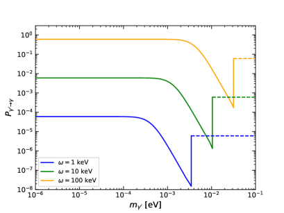
In this section, we show some analytical results for the dark vector-photon conversion probability to directly see how the probability is enhanced by a strong magnetic field. Since both modes of dark vector obey the same equations of motion (40), we will focus on the parallel mode below. The dark vector-photon conversion probability in the weak-mixing limit is given by
| (54) | |||||
where . We plot as a function of and in Fig. 13. In both plots, we take G and . As shown in the left plot of Fig. 13, the probability is a constant in the limit of low dark vector mass, eV at frequencies keV and NS radius km. Due to the term in the exponent of Eq. (54), as further increases, the probability is suppressed and oscillates around a constant, which is represented by the dashed line in the left plot. In the right plot we show the probability as a function of , the angle between the direction of propagation and the magnetic field, with eV.
For small values of , the oscillation term can be neglected and the conversion probability is approximated as
| (55) |
Averaged over , the probability can be parametrized as
| (56) |
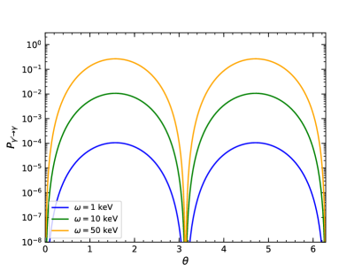
Note that we have used the -averaged probability in our calculations for the luminosity and spectrum. In the presence of an inhomogeneous external field, the probability is proportional to for the dark vector-to-photon conversion Fortin2019JCAP , but is inversely proportional to the frequency in the zero background field limit Masso2006PRL ; Ahlers2007PRD ; Ahlers2008PRD . Furthermore, when the external field is removed, the conversion probability approaches zero in the limit of low dark vector mass since in this case the probability is proportional to Masso2006PRL ; Ahlers2007PRD ; Ahlers2008PRD . However, for the case of an inhomogeneous external field, the dark vector-to-photon conversion probability dose not depend on in the low dark vector mass limit Fortin2019JCAP , which also appears in the axion-photon conversion Buschmann2021PRL .
Appendix D Dark vector emission in strong degenerate plasma
For the nucleon-nucleon bremsstrahlung emission of dark vectors in the NS core, we can safely assume a degenerate limit because of in the core of the NS. Let us first consider the process , the dark vector energy emission rate is given by the formula (6). Multiply the equation by one in the form Harris2020JCAP
| (57) | ||||
where and and are the Fermi momenta for neutron and proton, respectively, and has been used. The squared matrix can be expanded as
| (58) |
where for matrix (9) and (11). The energy emission rate (6) can be written as
| (59) |
where the energy integral is
| (60) |
after using . In the strong degeneracy limit , which is a good approximation for the processes taking place in the NS core, the energy integral is given by Iwamoto2001PRD
| (61) |
The angular integral is given by
| (62) | |||||
The dark vector momentum has been neglected in the momentum-conserving -function. Since the squared matrix element is in general a function of the momentum transfer and , we can convert the integral to and by inserting the unity Fortin2021
| (63) |
into the right-hand side of Eq. (62). We can eliminate , , and one by one with the aid of the three 3-momentum-conserving -functions. Then
| (64) | |||||
where we have relabeled as . In order to evaluate the integration, we choose the spherical coordinates to expand the three vectors as
| (65) |
Namely, lies along the axis, lies in the plane, and points to an arbitrarily direction. Then we have
| (66) | |||||
| (67) | |||||
| (68) |
The -functions in Eq. (64) indicate and
| (69) |
We see that the term proportional to does not contribute. This is the consequence of strong degeneracy limit.
The -functions in Eq. (64) can be written as
| (70) | |||||
| (71) | |||||
| (72) |
with the definitions , , and , and
| (73) |
Using the above relations, the integration (64) can be simplified as
| (74) |
with the constraints on the parameters and .
Similarly, for the process the angular integral is given by
| (75) |
Appendix E Remarks on OPE approximation
In order to realistically determine the production rate of new bosons (e.g. axion or dark vector) from nucleon-nucleon bremsstrahlung processes, the simplified treatment based on one-pion exchange and the use of the Born approximation for the nucleon-nucleon interaction was originally introduced in Refs. Friman1979APJ ; Iwamoto1984PRL ; Brinkmann1988PRD ; Turner1989PRD ; Carena1989PRD . It has been realized in the literature Hanhart2001PLB ; Schwenk2004PLB ; Rrapaj2016PRC ; Chang2018JHEP ; Carenza2019JCAP that such a simplified method ignores some relevant effects such as the multiple nucleon scatterings, and leads to a larger emission rate and thus a stronger constraint on the coupling.
One way to go beyond the OPE approximation has been performed in Refs. Hanhart2001PLB ; Schwenk2004PLB by including a nonperturbative treatment of the two-nucleon scattering in the soft-radiation approximation. It was found that for the range of conditions encountered in a NS, this treatment results in an approximate modification of the axion emissivity by a factor of when compared with the OPE results Beznogov2018PRC . Using the soft-radiation approximation, Ref. Rrapaj2016PRC calculated the dark vectors emissivity from a supernova and found a factor of 10 decrease in the emission rate. Reference Carenza2019JCAP refined the calculation based on the OPE approximation by systematically taking into account the effects that had been neglected previously, including the contribution of the two-pions exchange, effective in-medium nucleon masses and multiple nucleon scatterings. They found that the axion emissivity from a supernova was reduced by with respect to the basic OPE calculation. From these results we observe that the reduction of emissivity depends on the condition of matter. For the highly compressed matter in a NS, the emissivity is reduced by a factor of 4 with respect to the OPE approximation, while the factor can be up to 10 for the dilute plasma in a supernova.
Further improvement of the soft-radiation approximation can be made by including the many-body effects, such as the Landau-Pomeranchuk-Migdal (LPM) suppression Landau1953 ; Migdal1956PR owing to multiple scatterings in the medium. It has been shown in Ref. Dalen1003PRC that the LPM suppression of soft radiations increases with temperature and becomes relevant for MeV, above which the energy of the emitted boson is less than the nucleon decay width. Thus, the LPM effect is of particular importance for radiation in a supernova, but it becomes insignificant for the isolated NSs with a core temperature keV.
References
- (1) Planck Collaboration, Planck 2015 results, Astron. Astrophys. 594, A13 (2016).
- (2) B. W. Lee and S. Weinberg, Cosmological Lower Bound on Heavy-Neutrino Masses, Phys. Rev. Lett. 39, 165 (1977).
- (3) P. Hut, Limits on masses and number of neutral weakly interacting particles, Phys. Lett. 69B 85 (1977).
- (4) XENON Collaboration, Dark Matter Search Results from a One Ton-Year Exposure of XENON1T, Phys. Rev. Lett. 121, 111302 (2018).
- (5) Fermi LAT Collaboration, Searching for Dark Matter Annihilation from Milky Way Dwarf Spheroidal Galaxies with Six Years of Fermi Large Area Telescope Data, Phys. Rev. Lett. 115, 231301 (2015).
- (6) B. Holdom, TWO U(1)’S AND CHARGE SHIFTS, Phys. Lett. B 166, 196 (1986).
- (7) C.-W. Chiang and B.-Q. Lu, Evidence of a simple dark sector from XENON1T excess, Phys. Rev. D 102, 123006 (2020).
- (8) M. Ibe, A. Kamada, S. Kobayashi, T. Kuwahara and W. Nakano, Ultraviolet completion of a composite asymmetric dark matter model with a dark photon portal, JHEP 03, 173 (2019).
- (9) K. R. Dienes, C.F. Kolda, and J. March-Russell, Kinetic mixing and the supersymmetric gauge hierarchy, Nucl. Phys. B 492, 104 (1997).
- (10) A. Lukas and K.S. Stelle, Heterotic anomaly cancellation in five-dimensions, JHEP 01, 010 (2000).
- (11) R. Blumenhagen, G. Honecker, and T. Weigand, Loop-corrected compactifications of the heterotic string with line bundles, JHEP 06, 020 (2005).
- (12) S. A. Abel, M.D. Goodsell, J. Jaeckel, V. V. Khoze, and A. Ringwald, Kinetic Mixing of the Photon with Hidden U(1)s in String Phenomenology, JHEP 07, 124 (2008).
- (13) C. P. Burgess, J. P. Conlon, L. Y. Hung, C.H. Kom, A. Maharanad, and F. Quevedo, Continuous Global Symmetries and Hyperweak Interactions in String Compactifications, JHEP 07, 073 (2008).
- (14) M. Goodsell, J. Jaeckel, J. Redondo, and A. Ringwald, Naturally Light Hidden Photons in LARGE Volume String Compactifications, JHEP 11, 027 (2009).
- (15) C. Burrage, J. Jaeckel, J. Redondoa, and A. Ringwald, Late time CMB anisotropies constrain mini-charged particles, JCAP 11, 002 (2009).
- (16) M. Cicoli, M. Goodsell, J. Jaeckel and A. Ringwald, Testing String Vacua in the Lab: From a Hidden CMB to Dark Forces in Flux Compactifications, JHEP 07, 114 (2011).
- (17) M. Fabbrichesi, E. Gabrielli, and G. Lanfranchi, The Dark Photon, arXiv:2005.01515.
- (18) J.D. Bjorken, R. Essig, P. Schuster, and N. Toro, New Fixed-Target Experiments to Search for Dark Gauge Forces, Phys. Rev. D 80, 075018 (2009).
- (19) J.B. Dent, F. Ferrer and L.M. Krauss, Constraints on Light Hidden Sector Gauge Bosons from Supernova Cooling, arXiv:1201.2683.
- (20) D. Kazanas, R. N. Mohapatra, S. Nussinov, V. L. Teplitz, and Y. Zhang, Supernova Bounds on the Dark Photon Using its Electromagnetic Decay, Nucl. Phys. B 890, 17 (2014).
- (21) E. Rrapaj and S. Reddy, Nucleon-nucleon bremsstrahlung of dark gauge bosons and revised supernova constraints, Phys. Rev. C 94, 045805 (2016).
- (22) J. H. Chang, R. Essig, and S. D. McDermott, Revisiting Supernova 1987A constraints on dark photons, JHEP 01, 107 (2017).
- (23) E. Hardy and R. Lasenby, Stellar cooling bounds on new light particles: plasma mixing effects, JHEP 02, 033 (2017).
- (24) W. DeRocco, P. W. Graham, D. Kasen, G. M.-Tavaresa, and S. Rajendran, Observable signatures of dark photons from supernovae, JHEP 02, 171 (2019).
- (25) D. K. Hong, C. S. Shin, and S. Yun, Cooling of young neutron stars and dark gauge bosons, arXiv:2012.05427.
- (26) H. An, M. Pospelov, and J. Pradler, New stellar constraints on dark photons, Phys. Lett. B 725, 190-195 (2013).
- (27) H. An, M. Pospelov, and J. Pradler, Dark Matter Detectors as Dark Photon Helioscopes, Phys. Rev. Lett. 111, 041302 (2013).
- (28) N. Iwamoto, Axion Emission From Neutron Stars, Phys. Rev. Lett. 53, 1198 (1984).
- (29) D. E. Morris, Axion mass limits may be improved by pulsar x-ray measurements, Phys. Rev. D 34, 843 (1986).
- (30) R. P. Brinkmann and M. S. Turner, Numerical rates for nucleon-nucleon, axion bremsstrahlung, Phys. Rev. D 38, 2338 (1988).
- (31) N. Iwamoto, Nucleon-nucleon bremsstrahlung of axions and pseudoscalar particles from neutron-star matter, Phys.Rev.D 64, 043002 (2001).
- (32) D. Lai and J. Heyl, Probing axions with radiation from magnetic stars, Phys.Rev.D 74, 123003 (2006).
- (33) J.-F. Fortin and K. Sinha, Constraining Axion-Like-Particles with Hard x-ray Emission from Magnetars, JHEP 06, 048 (2018).
- (34) A. Sedrakian, Axion cooling of neutron stars, Phys. Rev. D 93, 065044 (2016).
- (35) A. Sedrakian, Axion cooling of neutron stars. II. Beyond hadronic axions, Phys. Rev. D 99, 043011 (2019).
- (36) P. Carenza, T. Fischer, M. Giannotti, G. Guo, G. Martinez-Pinedo, and A. Mirizzi, Improved axion emissivity from a supernova via nucleon-nucleon bremsstrahlung, JCAP 10, 016 (2019).
- (37) S. P. Harris, J.-F. Fortin, K. Sinhac, and M. G. Alford, Axions in neutron star mergers, JCAP 07, 023 (2020).
- (38) M. Buschmann, R. T. Co, C. Dessert, and B. R. Safdi, Axion Emission Can Explain a New Hard x-ray Excess from Nearby Isolated Neutron Stars, Phys. Rev. Lett. 126, 021102 (2021).
- (39) L. B. Leinson, Constraints on axions from neutron star in HESS J1731-347, J. Cosmol. Astropart. Phys. 11 (2019) 031.
- (40) L. B. Leinson, Impact of axions on the Cassiopea A neutron star cooling, J. Cosmol. Astropart. Phys. 09, 001 (2021).
- (41) J.-F. Fortin, H.-K. Guo, S. P. Harris, E. Sheridan, and K. Sinha, Magnetars and Axion-like Particles: Probes with the Hard x-ray Spectrum, arXiv:2101.05302.
- (42) A. Davidson, B-L as the fourth color within an mode, Phys. Rev. D 20, 776 (1979).
- (43) R. E. Marshak and R. N. Mohapatra, Quark-lepton symmetry and as the generator of the electroweak symmetry group, Phys. Lett. 91B, 222 (1980).
- (44) R. N. Mohapatra and R. E. Marshak, Local Symmetry of Electroweak Interactions, Majorana Neutrinos and Neutron Oscillations, Phys. Rev. Lett. 44, 1316 (1980); Erratum, Phys. Rev. Lett. 44, 1644 (1980).
- (45) A. Davidson and K. C. Wail, Universal Seesaw Mechanism? Phys. Rev. Lett. 59, 4 (1987).
- (46) J. C. Montero and V. Pleitez, Gauging U(1) symmetries and the number of right-handed neutrinos, Phys. Lett. B 03, 065 (2009).
- (47) E. Ma and R. Srivastava Dirac or Inverse Seesaw Neutrino Masses with Gauge Symmetry and Flavour Symmetry, Phys. Lett. B 12, 049 (2014).
- (48) C. Dessert, J. W. Foster, and B. R. Safdi, Hard x-ray Excess from the Magnificent Seven Neutron Stars, Astrophys. J. 904, 42 (2020).
- (49) J.-F. Fortin and K. Sinha, Photon-dark photon conversions in extreme background electromagnetic fields, J. Cosmol. Astropart. Phys. 11, 020 (2019).
- (50) D. Page, 2016, NSCool: Neutron star cooling code, Astrophysics Source Code Library, ascl:1609.009 [http://www.astroscu.unam.mx/neutrones/NSCool/].
- (51) J. Buchner, UltraNest – a robust, general purpose Bayesian inference engine, arXiv:2101.09604 [https://johannesbuchner.github.io/UltraNest/index.html].
- (52) A. Potekhin, D. Zyuzin, D. Yakovlev, M. Beznogov, and Y. Shibanov, Thermal luminosities of cooling neutron stars, Mon. Not. R. Astron. Soc. 496, 5052 (2020).
- (53) B. L. Friman and O. V. Maxwell, Neutrino emissivities of neutron stars., Astrophys. J. 232, 541 (1979).
- (54) M. V. Beznogov, E. Rrapaj, D. Page, and S. Reddy, Constraints on Axion-like Particles and Nucleon Pairing in Dense Matter from the Hot Neutron Star in HESS J1731-347, Phys. Rev. C 98, 035802 (2018).
- (55) C. Hanhart, D. R. Phillips, and S. Reddy, Neutrino and axion emissivities of neutron stars from nucleon-nucleon scattering data, Phys. Lett. B499, 9 (2001).
- (56) A. Akmal, V. R. Pandharipande and D. G. Ravenhall, Equation of state of nucleon matter and neutron star structure, Phys. Rev. C 58, 1804 (1998).
- (57) H.-Y. Chiu and E. E. Salpeter, Surface x-ray emission from neutron stars, Phys. Rev. Lett. 12, 413 (1964).
- (58) J. N. Bahcall and R. A. Wolf, Neutron stars. I. Properties at absolute zero temperature, Phys. Rev. 140, B1445 (1965).
- (59) J. N. Bahcall and R. A. Wolf, Neutron stars. II. Neutrino-cooling and observability, Phys. Rev. 140, B1452 (1965).
- (60) O.V. Maxwell, Neutrino emission properties in hyperon populated neutron stars, Astrophys. J. 316, 691 (1987).
- (61) D. G. Yakovlev, A. D. Kaminker, O. Y. Gnedin, and P. Haensel, Neutrino emission from neutron stars, Phys. Rep. 354, 1 (2001).
- (62) J. M. Lattimer, C. J. Pethick, M. Prakash, and P. Haensel, Direct URCA process in neutron stars, Phys. Rev. Lett. 66, 2701 (1991).
- (63) A.M. Beloborodov and X. Li, Magnetar heating, Astrophys. J. 833, 261 (2016).
- (64) D.G. Yakovlev and K.P. Levenfish, Modified URCA process in neutron star cores, Astron. Astrophys. 297, 717 (1995).
- (65) G. G. Raffelt, Stars as Laboratories for Fundamental Physics, (University of Chicago Press, 1996).
- (66) M. H. van Kerkwijk and D. L. Kaplan, Timing the Nearby Isolated Neutron Star RX J1856.5–3754, Astrophys. J. 673, L163 (2008).
- (67) F. M. Walter, T. Eisenbei, J. M. Lattimer, B. Kim, V. Hambaryan, and R. Neuhuser, Revisiting the Parallax of the Isolated Neutron Star RX J185635-3754 Using HST/ACS Imaging, Astrophys. J. 724, 669 (2010).
- (68) A summary of the observed NSs’ information can be found on the website: http://www.ioffe.ru/astro/NSG/thermal/cooldat.html.
- (69) F. Haberl, The magnificent seven: magnetic fields and surface temperature distributions, Astrophys. Space Sci. 308, 181 (2007).
- (70) G. E. P. Box and G. C. Tiao, Bayesian Inference in Statistical Analysis, A Wiley-Interscience publication, (1992).
- (71) W. C. G. Ho, D. L. Kaplan, P. Chang, M. van Adelsberg and A. Y. Potekhin, Magnetic hydrogen atmosphere models and the neutron star RX J1856.5-3754, Mon. Not. Roy. Astron. Soc. 375 821-830 (2007).
- (72) R. P. Mignani, D. Vande Putte, M. Cropper, R. Turolla, S. Zane, L. J. Pellizza, L. A. Bignone, N. Sartore, A. Treves, The birthplace and age of the isolated neutron star RX J1856.5-3754, Mon. Not. Roy. Astron. Soc. 429, 4 (2013).
- (73) T. Yoneyama, K. Hayashida, H. Nakajima, S. Inoue, and H. Tsunemi, Discovery of a keV-x-ray Excess in RX J1856.5–3754, Publ. Astron. Soc. Japan 69, 50 (2017).
- (74) J. Skilling, Nested Sampling, AIP Conference Proceedings 735, 395 (2004).
- (75) W. A. Rolke, A. M. Lopez, and J. Conrad, Limits and confidence intervals in the presence of nuisance parameters, Nucl. Instrum. Methods Phys. Res., Sect. A 551, 493 (2005).
- (76) D.J. Fixsen, E.S. Cheng, J.M. Gales, John C. Mather, R.A. Shafer, and E.L. Wright, The Cosmic Microwave Background spectrum from the full COBE FIRAS data set, Astrophys. J. 473, 576 (1996).
- (77) A. Caputo, H. Liu, S. Mishra-Sharma, and J. T. Ruderman (2020b), Dark Photon Oscillations in Our Inhomogeneous Universe, Phys. Rev. Lett. 125, 221303 (2020).
- (78) A. A. Garcia, K. Bondarenko, S. Ploeckinger, J. Pradler, and A. Sokolenko (2020), Effective photon mass and (dark) photon conversion in the inhomogeneous Universe, JCAP 10, 011 (2020).
- (79) S. D. McDermott and S. J. Witte, Cosmological evolution of light dark photon dark matter, Phys. Rev. D 101, (2020) 063030.
- (80) J. Jaeckel and S. Roy, Spectroscopy as a test of Coulomb’s law: A Probe of the hidden sector, Phys. Rev. D 82 125020 (2010).
- (81) M. Betz, F. Caspers, M. Gasior, M. Thumm, and S.W. Rieger, First results of the CERN Resonant Weakly Interacting sub-eV Particle Search (CROWS), Phys. Rev. D 88, 075014 (2013).
- (82) A. O. Sushkov, W.J. Kim, D.A.R. Dalvit, and S.K. Lamoreaux, New experimental limits on non-newtonian forces in the micrometer range, Phys. Rev. Lett. 107, 171101 (2011).
- (83) J. Murata and S. Tanaka, Review of short-range gravity experiments in the LHC era, Class. Quant. Grav. 32, 033001 (2015).
- (84) Y.-J. Chen, W. K. Tham, D. E. Krause, D. Lopez, E. Fischbach, and R. S. Decca, Stronger Limits on Hypothetical Yukawa Interactions in the 30–8000 nm Rang, Phys. Rev. Lett. 116, 221102 (2016).
- (85) H. An, M. Pospelov, J. Pradler, and A. Ritz, New limits on dark photons from solar emission and keV scale dark matter, Phys. Rev. D 102, 115022 (2020).
- (86) XENON Collaboration, Excess electronic recoil events in XENON1T, Phys. Rev. D 102, 072004 (2020).
- (87) PandaX-4T Collaboration, Dark Matter Search Results from the PandaX-4T Commissioning Run, arXiv:2107.13438.
- (88) K. Oh et al., The 105-Month Swift-BAT All-sky Hard x-ray Survey Astrophys. J. 235, 4 (2018).
- (89) R. Krivonos, Recent results from the INTEGRAL hard x-ray surveys, Mem. S. A. It. 90, 286 (2019).
- (90) E. Braaten and D. Segel, Neutrino energy loss from the plasma process at all temperatures and densities, Phys. Rev. D 48, 1478 (1993).
- (91) J. P. Blaizot, E. Iancu, and A. Rebhan, Approximately self-consistent resummations for the thermodynamics of the quark-gluon plasma: Entropy and density, Phys. Rev. D 63 065003 (2001).
- (92) G. Raffelt and L. Stodolsky, Mixing of the Photon with Low Mass Particles, Phys. Rev. D 37, 1237 (1988).
- (93) J. S. Heyl and L. Hernquist, Birefringence and dichroism of the QED vacuum, J. Phys. A 30, 6485 (1997).
- (94) A. Y. Potekhin, D. Lai, G. Chabrier, and W. C. G. Ho, Electromagnetic polarization in partially ionized plasmas with strong magnetic fields and neutron star atmosphere models, Astrophys. J. 612, 1034 (2004).
- (95) E. Masso and J. Redondo, Compatibility of CAST search with axion-like interpretation of PVLAS results, Phys. Rev. Lett. 97, 151802 (2006).
- (96) M. Ahlers, H. Gies, J. Jaeckel, J. Redondo, and A. Ringwald, Light from the hidden sector, Phys. Rev. D 76, 115005 (2007).
- (97) M. Ahlers, H. Gies, J. Jaeckel, J. Redondo, and A. Ringwald, Laser experiments explore the hidden sector, Phys. Rev. D 77, 095001 (2008).
- (98) M.S. Turner, Axions, SN 1987a and One Pion Exchange, Phys. Rev. D 40, 299 (1989).
- (99) M. Carena and R.D. Peccei, The Effective Lagrangian for Axion Emission From SN1987A, Phys. Rev. D 40, 652 (1989).
- (100) A. Schwenk, P. Jaikumar, and C. Gale, Neutrino bremsstrahlung in neutron matter from effective nuclear interactions, Phys. Lett. B584, 241 (2004).
- (101) J. H. Chang, R. Essig, and S. D. McDermott, Supernova 1987A Constraints on Sub-GeV Dark Sectors, Millicharged Particles, the QCD Axion and an Axion-like Particle, JHEP 09, 051 (2018).
- (102) L. Landau and I. Pomeranchuk, Electron cascade process at very high-energies, Dokl. Akad. Nauk Ser. Fiz. 92, 735 (1953).
- (103) A. B. Migdal, Bremsstrahlung and pair production in condensed media at high energies, Phys. Rev. 103, 1811 (1956).
- (104) E. van Dalen, A. Dieperink, and J. Tjon, Neutrino emission in neutron stars, Phys. Rev. C 67, 065807 (2003).