[1]\fnmJozef \surHanč
[1]\orgdivInstitute of Physics, \orgnameP.J. Šafárik University, \orgaddress\streetPark Angelinum 9, \cityKošice, \postcode04001, \countrySlovakia
2]\orgdivInstitute of Mathematics, \orgnameP.J. Šafárik University, \orgaddress\streetJesenná 5, \cityKošice, \postcode04001, \countrySlovakia
Probability distributions and calculations for Hake’s ratio statistics in measuring effect size
Abstract
Ratio statistics and distributions play a crucial role in various fields, including linear regression, metrology, nuclear physics, operations research, econometrics, biostatistics, genetics, and engineering. In this work, we examine the statistical properties and probability calculations of the Hake normalized gain as a measure of effect size and educational effectiveness in physics education. Leveraging existing knowledge about the Hake ratio as a ratio of normal variables and utilizing open data science tools, we developed two novel computational approaches for computing ratio distributions. Our pilot numerical study demonstrates the speed, accuracy, and reliability of calculating ratio distributions through (1) DE quadrature with/without barycentric interpolation, a very quick and efficient quadrature method, and (2) a 2D vectorized numerical inversion of characteristic functions, which offers broader applicability by not requiring knowledge of PDFs or the independence of ratio constituents. These numerical explorations not only deepen the understanding of the Hake ratio’s distribution but also showcase the efficiency, precision, and versatility of our proposed methods, making them highly suitable for fast data analysis based on exact probability ratio distributions. This capability has potential applications in multidimensional statistics and uncertainty analysis in metrology, where precise and reliable data handling is essential.
keywords:
Ratio statistics, Hake normalized gain, Effect size, Exact probability distributions, Integral transforms, Numerical computation, Double exponential quadrature1 Introduction
Today, ratio statistics and their distributions play an essential role not only in linear regression theory and metrology but also in a broad range of applications. According to several works [39, 44, 45, 6, 48], examples include nuclear physics (mass-to-energy ratios), operations research and engineering (safety factors in design, signal-to-noise ratios, radar distributions), econometrics (economic indicators), biostatistics (enzyme activity, red blood cell lifespan, medical study ratios), genetics (Mendelian inheritance ratios), and the food and pharmaceutical industries (digestibility measures, component ratios in foods or drugs), as well as meteorology (target-to-control precipitation ratios) and environmental science (environmental concentrations and loads).
Focusing on the ratio of normal variables, [12] points to the need to examine and apply this distribution in fields such as cytometry, physiology, risk analysis, and DNA microarrays. In this paper, we will describe and examine another useful and important application: ratios used in social and educational sciences as statistical measures of effect size (ES) for assessing intervention improvements, either pre- and post-intervention or between control and experimental groups.
In social, behavioral sciences, medicine and generally in education, one of the most popular and standard measures of effect size (ES),is the so-called Cohen’s statistical measure and its sample based estimator [7, 23]:
| (1.1) |
where are the average relative scores (in %) of a given group of participants on a diagnostic measurement tool, such as a standardized didactic test; represent the population mean scores , and are the population standard deviations of the score and its sample version, respectively.
Remark 1.
Even research and the publication of statistical analysis and inference dealing with subjective, repeated measurements in the aforementioned fields, as well as statistical education, require effect size reporting [23, 3, 10].
In physics education and physics education research (PER), for over 25 years [46, 41], another fundamental ratio as an ES measure has been used:
| (1.2) |
where .
This ratio, also known as the average normalized gain, was introduced by R. Hake [24] to measure understanding of key physics concepts in mechanics and other fields through a specialized type of research-based standardized didactic test, known as concept inventories [9]. In the context of PER, Hake’s ratio is widely used in the physics education community as a statistical measure of effect size and educational effectiveness, interpreting it as an indicator of the quality (effectiveness) of instruction or educational activities in introductory physics courses.
The main goal of this article is to examine the statistical properties and methods for probabilistic computations of the Hake normalized gain, which statistics offers from analytical, empirical, computational, and numerical perspectives to provide valuable insights and enhance understanding of the ratio in real data applications.
The article is structured as follows. Since the Hake ratio is a ratio of correlated normal random variables, in Section 2, we revisit all relevant knowledge on basic statistical properties. For better clarity, the theoretical results are simultaneously applied and illustrated using hypothetical or real datasets from PER. In Section 3, we address recent computational and numerical approaches for probability calculations, mainly connected to integral transforms (i.e., Mellin, Fourier) and special functions (i.e., confluent hypergeometric functions), including our two proposed methods, all of which are compared in a pilot numerical study described in Section 4.
In conclusion, we analyze the significance of our statistical findings from the perspectives of both the PER community and statistics itself. We also address the implications and potential future applications, which extend beyond the specific ratio of normal variables to enable rapid data analysis based on exact probability distributions for ratios of arbitrary continuous random variables. This capability is promising for fields such as multidimensional statistics and uncertainty analysis in metrology, where precise data handling is essential. For clarity, the proofs, detailed formulas, and tools used are provided in the appendices.
2 Statistical properties of Hake’s ratio
2.1 Context and background
When Hake introduced the normalized gain in his landmark meta-analysis article [24] to measure instruction quality, he also used empirical data from 62 introductory physics courses (, average participants per course), as shown in the plot on the left in Fig. 1. This visualization also provided an important geometric interpretation with some consequences about used teaching methods.
At point , representing the results of a particular course, the Hake ratio is the tangent of the angle formed by the line connecting point with point . It was observed that courses taught with traditional teaching methods achieved results up to , concentrated around a slope of , while courses with interactive teaching methods fell within the range between lines with slopes from 0.3 to 0.6, centered around a slope of .

Hake’s statistic was and is understood almost exclusively as an empirical measure, representing the practical relative improvement of a group of students after instruction, with recurring discussions about the appropriateness and usefulness of its application [25, 9].
From a statistical perspective, however, only a few articles address the statistical properties of Hake’s statistic and its theoretical or empirical validation. For example, in [8], the author provides empirical evidence showing that real data does not reject the hypothesis of a normal distribution. Regarding theoretical statistical considerations, to the best of our knowledge, only one article [5] attempts such an approach, but a significant weakness of this derivation is its lack of alignment with existing statistical literature.
Therefore, our main goal is to examine the statistical properties and probabilistic computation methods for the Hake normalized gain, offering comprehensive, mutually supportive analytical, empirical, computational, and numerical perspectives to deepen understanding and insights into this ratio in real data applications.
2.2 Analytic form and shape of the distribution
First of all, as stated in the following proposition, using elementary statistical properties of distributions and their moments, we can easily prove that Hake’s ratio is a ratio of two correlated normal random variables (RVs).
Proposition 1 (Hake’s ratio distribution).
Hake’s normalized gain , given by (1.2) is a ratio of correlated normal random variables and :
| (2.3) |
where
-
-
,
-
,
-
The symbol denotes a bivariate normal distribution with given parameters. Proofs of the proposition and remaining theorems are provided in Appendix A. Now, let us briefly summarize key results of the statistical literature about the analytical properties of this distribution, denoted as , and apply these findings to Hake’s ratio.
In [28], we can find the analytic forms for the PDF and CDF of the ratio (the CDF of the ratio , expressed via the bivariate normal integral, is again in Appendix A (Theorem 6).
Theorem 2 (PDF of [28]).
Let , . Then the PDF of is given by:
| (2.4) | ||||
where is the CDF of :
However, there also exists a much comprehensible analytical form, which is both clearer for theoretical study and easier for practical computational implementation.
Theorem 3 ([39, 49]).
For , there are constants and such that:
-
is distributed as ,
-
is distributed as , where
(2.5) -
, , ,
-
(2.6) -
where is Kummer’s confluent hypergeometric function [22].
A very surprising result of this theorem for non-statisticians is that it is not necessary to study the statistical properties of the ratio of correlated normal RVs. By using the presented Marsaglia "orthogonal" transformation, discovered even before Hinkley [38], it suffices to consider only the transformed ratio of independent normal RVs. The formally simpler expression in terms of allows for examining properties such as symmetry, modality, and monotonicity, as discussed in detail in [49].
Combining the results of Theorems 1 and 3 provides us the following corollary with the formulas for and related to Hake’s ratio.
Corollary 4 ( for Hake’s ratio).
An additional benefit of the transformation is that the modality, mathematically described by the number of solutions to , is directly determined by the values of the resulting parameters and . For example, it leads to a practical rule of thumb for any [38]:
Rule of Thumb: For the PDF of (and ) is unimodal,
for the PDF (and ) is bimodal.
In the "transition range" , the modality depends on and is determined by the modality curve (see Appendix A). Figure 2 illustrates the bimodal shape of for specific values of the original parameters, resulting in .

Remark 2.
Section 5 in [49] provides a rigorous procedure for dividing the plane into two regions by a modality curve given by , such that the PDF is unimodal for points on the left of that curve and bimodal on its right (Figure 2, right). Modern digital tools [19] allow very easily to create an interactive Jupyter notebook demonstrating the entire process as a virtual experiment in a visual and highly intuitive way.
2.3 Normal approximation of the distribution
Another surprising and statistically inconvenient property of the distribution of the ratio of two normal random variables and is its heavy-tailed nature and lack of finite moments. However, in the case of a unimodal shape, practical applications like Hake’s ratio [8] result in a distribution very close to a normal distribution.
When the means are positive, using a Taylor series expansion of the ratio around the point , the first-order term provides the mean approximation, and the second-order term approximates the variance [12, 39]. These "pseudo-moments" are given in the following expression (corresponding to the law of uncertainty propagation):
| (2.7) |
The conditions for such a reasonable approximation can be formulated numerically [39] and by the existence theorem [12]. This work also introduces a graphical tool, the ROC curve, which is useful for assessing the closeness of the distribution of a specific ratio to the proposed normal approximation.
The specific normal distribution approximation of Hake’s empirical distribution [8] can be seen in Figure 3.

Remark 3.
It appears that in statistical literature, the most cited source is [28], even it does not actually derive the analytical form but rather compares the exact distribution with its approximation. The derivation itself was already provided in an earlier work of [15]; therefore, in some resources, the ratio of normal RVs is referred to as Fieller’s distribution. It is also worth mentioning that the connection between as sufficient for studying the properties of suggested by [38] was not fully understood by [28], though this was later corrected in [29].
3 Numerical Calculations for the Ratio
3.1 Mellin Transform Approach via Convolution
As long-time, experienced users of R and Python for nearly every statistical purpose, we naturally expected an open-source package for calculating the PDF, CDF, approximations, or performing statistical inference related to the ratio of or . The third surprise for us was discovering that such a specialized package does not exist. The only available software is a nearly 20-year-old code from the previously mentioned study [39].
The choice of computational method and an appropriate digital tool for scientific computing is therefore left to the potential user. However, when dealing with the analytic formula — containing the hypergeometric confluent function — various computational issues may arise [33, 26]. Therefore, we decided to investigate more deeply the potential numerical approaches that would be suitable for ratio distributions.
As the first result of our research, we found an open-source solution capable of handling probabilistic and statistical computations for our ratio distribution. Specifically, a more general Python package, PaCAL (the Probabilistic CALculator) [35], is able to numerically perform arithmetic operations () on independent continuous random variables, running on Cython (a C-optimized version of Python). In exploring its documentation, we found that PaCAL computes the ratio distribution through the Mellin transform theory, using the Clenshaw-Curtis (CC) quadrature with barycentric interpolation (via Chebyshev polynomials) [31].
The Mellin transform, defined as [52]:
| (3.8) |
represents a powerful tool for studying the distribution of products, ratios, and, more generally, algebraic functions of independent RVs. Its significance is analogous to that of the Fourier integral transform, which is connected to the characteristic function effectively used for distributions of sums [52].
Arguably the most comprehensive handbook on the topic of the Mellin transform is Springer’s book [52]. The most comprehensive tables of properties and closed expressions for several integral transforms, including the Mellin transform, can be found in the Caltech Project, led by editor A. Erdélyi [13, 14].
It is worth noting that the Mellin transform exists for a real function that is defined and single-valued almost everywhere for and is absolutely integrable over the range . The Mellin transform can be extended [52] to the range . The importance of the Mellin transform in studying the product and ratio of independent random variables lies in the fact that they can be expressed using the so-called Mellin convolution.
Theorem 5 (Mellin convolution for product and ratio [52]).
Let and be independent continuous RVs with PDFs and . Then, the PDFs of the product and ratio and are given by:
| (3.9) |
For the ratio of independent random variables and , substituting the PDFs of and ,
into the Mellin convolution (3.9) gives us the PDF of the ratio distribution
| (3.10) |
At first glance, this integral appears significantly simpler compared to expression (2.6) in Theorem 3, which contains Kummer’s confluent hypergeometric function. However, by using tabulated expressions of the Mellin transform [13], the Mellin convolution integral (3.10) can be directly and analytically computed to yield a result identical to (2.6); see Appendix A.
In practice, however, the integral can be computed numerically using an appropriate numerical method, quadrature. The mentioned Cython PACAL package calculates such an integral using the CC quadrature with barycentric interpolation.
3.2 Fourier transform approach via characteristic function
The probability distribution of any real-valued RV is completely determined by its characteristic function , which is mathematically equivalent to the Fourier transform [51]. In many situations, the form of the characteristic function (CF) is analytically known or much simpler than the PDF or CDF of the RV.
In such cases, the characteristic function provides an alternative numerical method for effectively computing the PDF and CDF of the RV through the conceptually simple approach known as the numerical inversion of the characteristic function, which remains less widely known but has been periodically highlighted in research over the past 50 years (e.g., [11, 58, 60]). This computational approach is based on the numerical quadrature of the Gil-Pelaez inversion formulae [21]:
| (3.11) |
The current numerical inversion CF approach
Regarding ratios of RVs, the currently used characteristic function approach [61] is based on the logarithmic transformation and applies only to , which are independent non-negative RVs. For , , , and assuming we know the CFs of the log-transformed variables, the CF of the ratio is given by . Inverting the CF of the log-transformed ratio , we can then obtain the required distribution of the ratio . This approach can be successfully applied to model data with skewed distributions or distributions with heavy tails, where it is possible to compute exact distributions for likelihood ratio tests (LRT) statistics [62], or in more complex cases, in multivariate analysis for LRT statistics [16].
An approach via Mellin transform with CFs
In the case of independent RVs with values across the real line, however, a different approach is required. One straightforward option is to use the Mellin convolution (3.9) and substitute for PDFs of and using the inversion formula (3.11):
| (3.12) |
Numerically, we would generally have to tackle a 3D numerical quadrature, which would drastically increase the computational complexity of this task, making it realistically feasible only with high performance computing (HPC) on supercomputers.
The Broda-Kan approach
[4] proposed a different approach. They introduced an auxiliary random variable , which "linearizes" the problem of the CDF of the ratio in the sense that
Using an elementary identity [50] for the probability of a symmetric difference applied to the events , the CDF of the ratio is given by
Moreover, acknowledging the CF relation , authors derive a general inversion theorem for the CDF and PDF of the ratio of not necessarily independent variables, as detailed in Appendix A (Theorem 7). Here we will focus on the expression for the PDF
| (3.13) |
Considering for independent , i.e., , the PDF of ratio takes the simplified form
| (3.14) |
In this case, the PDF of the ratio of two independent variables is expressed as a 2D numerical CF inversion integral. With a suitable, sufficiently fast, and precise numerical quadrature, leveraging the fact that standard PCs have multiple CPUs and especially GPUs, parallel execution on CPUs or GPUs can make the computational task feasible even on the standard devices.
3.3 Double exponential quadrature
The result of our research and theoretical considerations in Sections 3.1 and 3.2 is that we now have two fundamentally suitable approaches to numerically compute the ratio of two independent continuous RVs and . Both approaches are applicable under very mild conditions, i.e., without the necessity of assuming that the RVs to be normally distributed. The first approach is the 1D Mellin convolution integral (3.9) using the PDFs of and . The second approach relies on knowing the CFs of and , involving the calculation of the 2D numerical CF inversion integral (3.14).
From a computational perspective, both integral transforms can be evaluated using any suitable numerical quadrature method. The open source package PaCAL [35] employs the very effective CC quadrature with barycentric interpolation based on Chebyshev polynomials for the numerical calculation of (3.9) [31].
We found that 2D numerical CF inversion integrals can be computed numerically using free MTB’s CharFunTool by [61] with the bivariate algorithm cf2Dist2D [see theoretical details in 42]. This algorithm also employs CC quadrature with barycentric interpolation in 2D and additionally offers a simple 2D trapezoidal rule (TR) quadrature as an alternative option.
It is important to note that the output of cf2Dist2D is the PDF of the bivariate distribution of the random vector , calculated from its bivariate CF by
| (3.15) |
To compute our 2D integral (3.14), it is sufficiently to choose , with the bivariate characteristic function The derivative of can be calculated symbolically or numerically. Key details of adjusting the authors’ numerical algorithm for calculating the integral (3.14) are provided in the Appendix (Numerical Quadrature Algorithm).
Regarding numerical quadrature, a very promising alternative to the CC algorithm is the double exponential (DE) quadrature [56, 43]. We remind only the core idea (for more details, see Remark 4), which lies in applying the simple trapezoidal rule to an integral transformed by a suitable DE transformation ():
so the trapezoidal rule is modified by introducing a weight function with a double-exponential decay rate Such DE transformations (three examples are in Table 1) make the trapezoidal rule optimally efficient, yielding exponentially fast and accurate results for a very broad class of functions (even with multiple singularities).
| DE transformation formulas |
|---|
Remark 4.
The DE quadrature was successfully applied in our study [26, see DE quadrature refs] to calculate the gamma difference distribution with unequal shape parameters through numerical integration of the classical convolution integral or the 1D numerical CF inversion integral. DE quadrature formulas have been proven optimal, achieving smaller errors than any other formula with the same average node count [55]. Although still less common in statistical applications, DE quadrature also has strong applications across fields such as molecular physics, fluid dynamics, boundary element methods, integral equations, ordinary differential equations, or complex indefinite and multiple integrals.
In the Scientific Python ecosystem, the DE quadrature can be seamlessly combined with barycentric interpolation-based Chebyshev polynomials (via the BarycentricInterpolator function from scipy). For open-source computational implementations, the sinh-sinh DE transformation is particularly suitable for the 1D Mellin convolution integral (3.9) in our case. This approach utilizes our Python implementation of the 1D DE quadrature [18], which is a modified Python version of the original C implementation by [47].
Additionally, we have developed a small Python package, Chebyshev.py, specifically tailored for our PDF calculations, enabling the combination of DE quadrature with barycentric interpolation. Regarding the 2D numerical CF inversion (3.14), we decided to adapt the Witkovský’s algorithmic approach for numerical inversion of bivariate CF. As a potential alternative, we also decided to explore MPFUN2020 library [1, 59], a thread-safe, arbitrary-precision Fortran package. This library includes a 2D implementation of the DE quadrature and supports its parallel execution on CPU/GPUs.
4 Open data tools numerical study
4.1 Setup, tools and conditions
For purposes of numerical study benchmarking chosen computational methods and digital tools, we use the open Jupyter interactive computing environment, combined with open-source tools like the computer algebra system SageMath as its kernel, enabling to work with multiple programming languages, such as Python and R, within a unified digital workspace. Additionally, systems like SageMath provide the computational power of traditional software without financial barriers, fostering accessibility and empowering research without the constraints of commercial software. A detailed list of the open digital tools used in our study is in Appendix B.
All computations were conducted on a PC with Windows 11 and a 12th Gen Intel(R) Core(TM) i7-12700K processor @ 3.60 GHz, featuring Intel(R) UHD Graphics 770, 8 performance cores, 20 threads, and 32 GB of RAM. The Python, Fortran, SageMath, and other free open software were installed from their official repositories, while MATLAB (MTB) computations were performed using the version R2023b as a kernel in our Jupyter environment [40].
4.2 Results and discussion
We conducted one numerical experiment for each available computational method and corresponding digital tool. Each experiment involved 3 runs, with each run containing 10 realizations of computing at 1000 points uniformly distributed over a chosen interval. This setup resulted in a total of calculations per experiment. Built-in commands or functions were used to measure the execution time of each experiment. To verify accuracy, we generated results using SageMath with quadruple precision (34 digits of accuracy) and cross-checked them by the arbitrary-precision C library Arb.
The benchmark results from each experiment include average runtime, runtime standard deviation, acceleration (relative to the SageMath analytic approach), and accuracy (maximum absolute error). The complete numerical study encompasses systematically carried-out 251 experiments (250 successful and 1 unsuccessful), with some chosen results summarized in Table 2, Figures 5, and 5. All resulting data and code, including 20 Jupyter notebooks, describing also our developments of algorithms in Python and MTB, are available at https://github.com/JupyterPER/HakeRatio.
The benchmark for specific methods and tools consists of:
-
•
13 experiments using the analytic expression (2.6) in SageMath via the fast_float routine (53-bit, to );
-
•
26 experiments using CC quadrature of the 1D Mellin convolution integral (3.9) in PaCAL, with and without Cython initialization (53-bit, to );
-
•
78 experiments using DE quadrature of the 1D Mellin convolution integral (3.9) in Python, with and without Numba, parallelization, barycentric interpolation (53-bit, to );
-
•
16 experiments using trapezoidal rule (TR) of the 2D numerical CF inversion integral (3.14) in Python (53-bit) dealing with different algorithms for an approximating integral sum (compiled in different Numba settings – with/without vectorization, parallization, symbolic/numerical derivative);
-
•
118 experiments using TR or CC quadrature (without/without vectorization, parallelization, symbolic/numerical derivative and various numbers of Chebyshev nodes; using built-in integrators and/or analytical implementations) of the 2D numerical CF inversion integral (3.14) in MTB (53-bit);
-
•
1 experiment using DE quadrature of the 2D numerical CF inversion integral (3.14) in Fortran via MPFUN (53-bit).
| Probability density function for ratio ( points over 6 interval of ) | ||||
|---|---|---|---|---|
| Method | Quadrature, Tool | Run (s) | Accel | Accur |
Kummer’s , Sage (fast_float, 53-bit)
|
e-04 | e-16 | ||
| Kummer’s , MTB (53-bit) | e-03 | e-16 | ||
| CC, PACAL (Cython, 53-bit) | e-04 | 240 | e-16 | |
| DE, Python (e-03) | e-02 | e-04 | ||
| DE, Python (Numba-par, e-15) | e-04 | e-16 | ||
| DE, Python (Numba-par, e-10) | e-04 | e-13 | ||
| DE, Python (Numba-par, e-03) | e-04 | e-04 | ||
| DE-CC(), (Numba, vect, e-06) | e-04 | e-09 | ||
| DE-CC(), (Numba, vect, e-15) | e-03 | e-16 | ||
| TR, Python (Numba-par, no vect) | e-01 | e-04 | ||
| TR, Python (Numba-par, vect) | e-01 | e-04 | ||
| BI, MTB (par, e-03) | e-00 | e-08 | ||
| BI-CC, MTB (par, e-03) | e-00 | e-08 | ||
| TR, MTB (par, no vect) | e-00 | e-04 | ||
| TR, MTB (no par, vect) | e-01 | e-04 | ||
| CC, MTB (no par, vect) | e-03 | e-02 | ||
| CC, MTB (no par, vect) | e-02 | e-02 | ||
| DE, Fortran (MPFUN2020) | — | — | — | |
| Abbr. par parallelization, vect vectorization, BI built-in integrator, MTB MATLAB | ||||
| the number of Chebyshev’s nodes in barycentric interpolation | ||||
In Table 2, we present a sample of deliberately selected experiments divided into three main groups based on the method of computing the ratio, each group clearly demonstrating the key results of our numerical study. Some of these results are also visualized in Figures 5 and 5.
As for the analytic formula (2.6), the built-in implementations of Kummer’s confluent hypergeometric function for computing the PDF of the ratio are highly accurate and reliable, which is not always the case for hypergeometric functions [33, 26]. Notably, the SageMath version is an order of magnitude faster (about 7x) than MTB, despite MTB’s reputation for numerical efficiency.
For the Mellin convolution integral, we conducted successful experiments in Python using the PACAL package and Python-based DE implementations. Both CC and DE quadrature methods, combined with high-performance compilers (Cython, Numba), achieved comparable speeds. While PACAL was the fastest, this excludes the 1-second initialization of the barycentric interpolant. Both quadratures delivered reliable results, with DE offering efficient accuracy control, where increasing accuracy by 12 orders of magnitude slows computation by less than one order of magnitude.
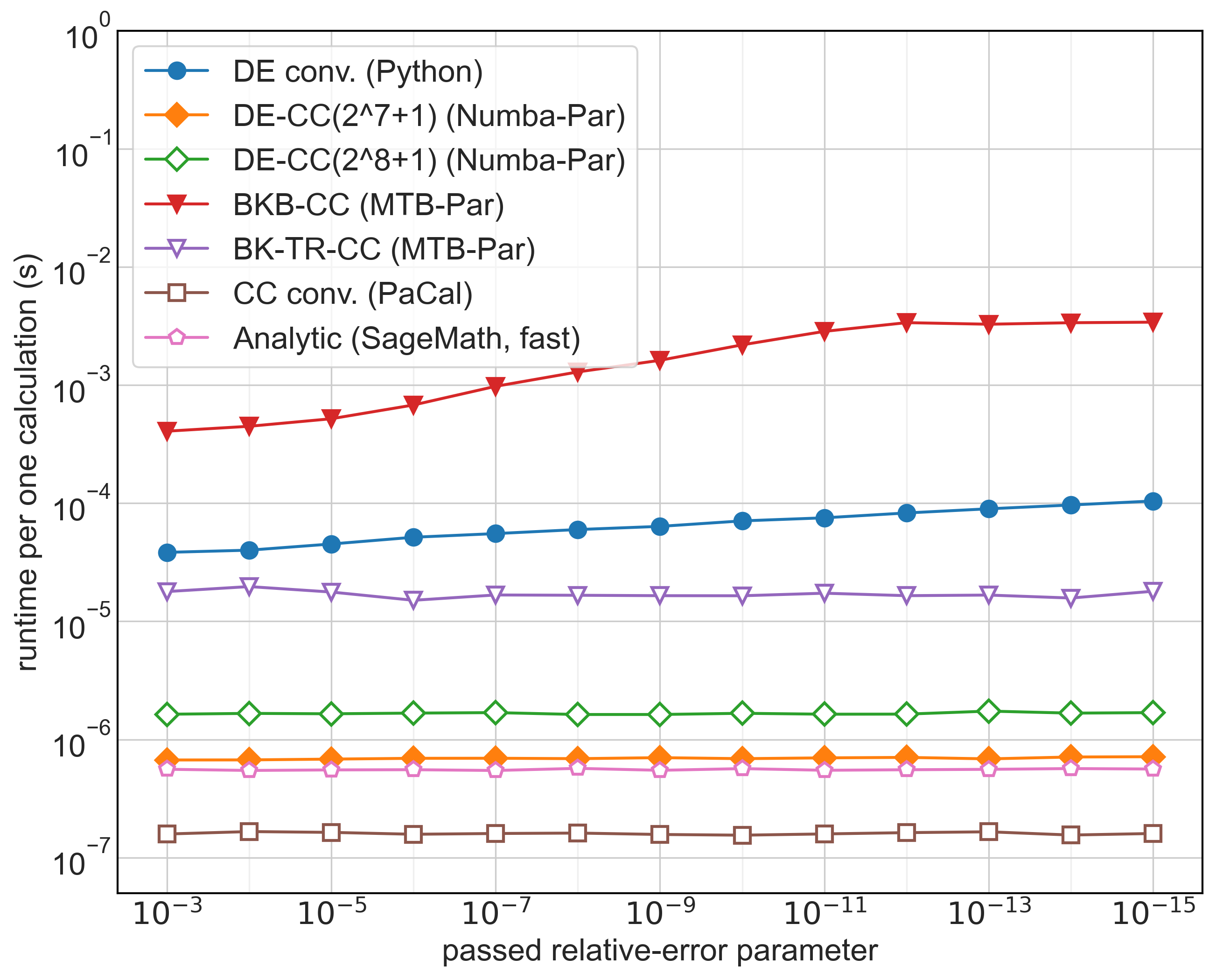

At first glance, our newly implemented DE quadrature combined with barycentric interpolation of adjustable accuracy appears to be several times slower. However, it is important to note that the built-in scipy implementation of the barycentric interpolator does not utilize process parallelization. Without parallelization, the speed of the DE quadrature alone is an order of magnitude lower. Ultimately, the use of Chebyshev interpolation accelerated the computation.
The majority of our numerical experiments were conducted using custom MTB and Python algorithms for the numerical inversion of the ratio via the Broda-Khan approach (3.14). While this 2D method is more computationally intensive, achieving speeds 2 orders of magnitude lower than the 1D Mellin convolution, the accuracy and performance are still practically acceptable. At more reduced accuracy, performance is comparable to 1D Python’s DE quadrature or MTB’s analytical computations.
In Python, parallelizing three nested loops (TR, Numba-par) improved 2D inversion speeds by 5-7x per loop, proportional to the number of cores. Without parallelization, the speed drops by 3 orders of magnitude. In MTB, full vectorization (TR, par vect) reduced computation time significantly (from 7.97 s to 0.19 s), proving much more efficient than MTB’s built-in parallelization. With barycentric interpolation, MTB is fast comparably to its analytical computations.
One set of experiments—the 2D-DE quadrature in the Fortran library MPFUN2020—was unsuccessful, with inconsistent results and calculation failures.111We attribute this not to the failure of method but to our limited familiarity with Fortran. Future solutions include collaborating with experts, improving our understanding, or rewriting the code in more familiar languages, potentially with AI assistance, as we did for Marsaglia’s C code.
5 Conclusions
In the first part of this article, we examined the statistical properties of Hake’s normalized gain, a ratio of two correlated normal random variables. In the PER community, where this measure was first introduced as an indicator of educational effectiveness, it has largely been used empirically. By referencing relevant statistical studies, we clarified its theoretical aspects and illustrated them with real data. The Hake distribution lacks moments (no mean or variance) and has heavy tails. However, in practice, it often approximates a normal distribution well.
Previous efforts to analyze its statistical properties, such as those by [5, 8], have remained primarily empirical, with minimal reflection on existing statistical literature or comments suggesting these properties are "quite messy" to present or study. To address this, we also provided 6 interactive Jupyter SageMath notebooks [19] at our GitHub that allow users to explore the properties of Hake’s distribution through virtual experimentation.
From a statistical standpoint, this first part also reviews the most relevant studies on the statistical properties of ratios of random variables (RVs), covering analytical forms, properties, and available software [39, 49], as well as numerical approximations [12]. Recognizing the lack of accessible software for ratio of normal variables, we decided to explore possibilities fo code into Python and R, much more widely used in current data science and statistics.
Obtained theoretical, empirical, and computational insights provided an essential foundation for the second part of the article. Using known analytic forms for the Hake ratio as a cross-check, we were able to develop two novel computational approaches for probability calculations of ratios: (1) the DE quadrature with or without barycentric interpolation for Mellin ratio convolution, and (2) a 2D vectorized version of the Broda-Khan numerical inversion based on the characteristic functions of ratio constituents. Both approaches can address not only Hake’s normalized gain but also ratios of independent or correlated random variables without normality assumptions. The entire process is documented, along with examples and codes, in an additional 8 Jupyter notebooks.
The speed, accuracy and reliability of results were tested in a pilot numerical case study (6 Jupyter notebooks with resulting data files). Using open digital tools and MTB, we show that our high-performance Python implementation (with Numba) of DE quadrature for Mellin ratio convolution achieves reliability and accuracy at least on par with the sophisticated Cython-based PaCAL package, with speeds comparable to C. Our approach, however, offers advantages in terms of easily adjustable error levels, allowing for speed improvements of up to threefold over PaCAL. Although preliminary, these findings are an important necessary first step toward developing a new Python or R package for the ratio of correlated normal distributions.
Our second proposed method, a vectorized and/or parallelized 2D Broda-Khan numerical CF inversion, broadens the scope of existing approaches for computing ratios. The first extension lies in its ability to effectively handle RVs with negative values. Furthermore, this method does not require knowledge of PDFs, as CFs alone are sufficient. It can even potentially be applied to correlated variables, further enhancing its versatility compared to the Mellin-transform approach.
While this 2D method is more computationally intensive, achieving speeds two orders of magnitude lower than the 1D Mellin convolution, its accuracy and performance remain practically acceptable. At reduced accuracy, its performance becomes comparable to 1D DE quadrature or analytically based computations. For future work, we strongly believe that successfully implementing a 2D version DE quadrature with CPU/GPU parallelization could lead to substantial speedups. This capability holds potential for rapid data analysis based on exact probability distributions of products and quotients of random variables in fields like measurement uncertainty analysis ior multidimensional statistics.
Acknowledgments This work was supported by the Slovak Research and Development Agency under the Contract No. APVV-21-0369, No. APVV-21-0216 and by the Slovak Scientific Grant Agency VEGA under grant VEGA 1/0585/24. We would also like to express our gratitude to Gabriel Semanišin from P.J. Šafárik University, for providing us with a one-year university license for MATLAB R2024b.
Appendix A Important formulas and proofs
Proof of Proposition 1 (Hake’s ratio distribution). In educational settings with groups ( or more), we can apply the central limit theorem for average scores , . The relations between parameters are direct consequences of basic properties of covariance and correlation [50].
Theorem 6 (The CDF of [28]).
Let , . Then the CDF of is given by:
| (A.16) | ||||
where denotes the standard bivariate normal integral:
| (A.17) |
Modality curve (defined by ). According to [39], the modality curve plotted in Figure 2 may be numerically approximated by ():
The coefficients were obtained using CAS Maple with 50 digits of accuracy.
Proof of the analytic form of the integral (3.9) (via the Mellin transform).
By changing to new variables and with the substitutions and , the Mellin convolution integral (3.9) transforms to the integral
Splitting the integral at zero and applying the Mellin transform, we obtain
There is a closed integral expression for this Mellin transform [eq. 6.3.(13), 13]:
where is the parabolic cylinder function and is the Hermite function [37]. Since the following relationship holds between the Hermite function and Kummer’s confluent hypergeometric function [22]:
we obtain the desired result (2.6):
Theorem 7 (The inversion theorem for ratio [4]).
If has a finite mean, is absolutely integrable, and 0 is not an atom of , then for the PDF and CDF are
| (A.18) |
and
| (A.19) |
whenever this integral converges absolutely.
Numerical 2D quadrature algorithm for integral (3.14).
The integral (3.14) can be rewritten in the following form corresponding to the 2D integral (3.15)
where and .
Then the 2D integral can be approximated by the trapezoidal rule integral sum [42] giving the PDF in vector of points
Using vectorization, vector and matrix representations, we can determine the ratio PDF (3.14) conceptually by the same algorithm as for bivariate PDF (3.15).
Appendix B Open digital tools
| Open digital tools | |
|---|---|
| Main Tools | SageMath [v. 10.3, 53], Python [v. 3.11.6, 57], Fortran [v. 2023, 30] |
| Numerical & scientific computing libraries | • NumPy [v. 1.19.1, 27]: Numerical Python library for fast vector computations • SciPy [v. 1.11.3, 34]: Fundamental Python library for scientific computing • GSL [v. 2.7.1, 20]: C, C++ numerical library for scientific computing • PaCAL [v. 1.6.1, 35]: Cython probabilistic calculator for arithmetics of i.r.v.’s • Arb [v. 2.16.0, 32]: C library for arbitrary-precision interval arithmetic using the midpoint-radius representation ("ball arithmetic") • Fortran-Magic [v. 0.9, 17]: Python library for executing Fortran code in Jupyter [59, MPFUN2020] • Jupyter-Matlab-Proxy [v. 0.15.3, 40]: Python library from MathWorks enabling MTB as a kernel for Jupyter. |
| High performance Python compilers | • Cython [v. 3.0.10, 2]: Optimizing static compiler translating Python into C code; also suitable for running C/C++ codes [39] • Numba [v. 0.59.1, 36]: JIT compiler translating Python into fast machine code; also suitable for GPU/CPU parallelism |
| \botrule | |
References
- \bibcommenthead
- Bailey and Borwein [2011] Bailey, D.H. and J.M. Borwein. 2011. High-precision numerical integration: Progress and challenges. J Symb Comput 46(7): 741–754. 10.1016/j.jsc.2010.08.010 .
- Behnel et al. [2011] Behnel, S. et al. 2011. Cython: The best of both worlds. Comput Sci Eng 13(2): 31–39. 10.1109/MCSE.2010.118 .
- Bowman [2017] Bowman, N.D. 2017. The Importance of Effect Size Reporting in Communication Research Reports. Communication Research Reports 34(3): 187–190. 10.1080/08824096.2017.1353338 .
- Broda and Kan [2016] Broda, S.A. and R. Kan. 2016. On distributions of ratios. Biometrika 103(1): 205–218. 10.1093/biomet/asv052 .
- Burkholder et al. [2020] Burkholder, E., C. Walsh, and N.G. Holmes. 2020. Examination of quantitative methods for analyzing data from concept inventories. Phys Rev Phys Educ Res 16(1): 010141. 10.1103/PhysRevPhysEducRes.16.010141 .
- Celano et al. [2014] Celano, G. et al. 2014. Statistical Performance of a Control Chart for Individual Observations Monitoring the Ratio of Two Normal Variables. Qual Reliab Eng Int 30(8): 1361–1377. 10.1002/qre.1558 .
- Cohen [1988] Cohen, J. 1988. Statistical Power Analysis for the Behavioral Sciences (2nd ed.). New York: Routledge.
- Coletta [2023] Coletta, V.P. 2023. Evidence for a normal distribution of normalized gains. Phys Rev Phys Educ Res 19(1): 010111. 10.1103/PhysRevPhysEducRes.19.010111 .
- Coletta and Steinert [2020] Coletta, V.P. and J.J. Steinert. 2020. Why normalized gain should continue to be used in analyzing preinstruction and postinstruction scores on concept inventories. Phys Rev Phys Educ Res 16(1): 010108. 10.1103/PhysRevPhysEducRes.16.010108 .
- Cumming and Calin-Jageman [2024] Cumming, G. and R. Calin-Jageman. 2024. Introduction to the New Statistics: Estimation, Open Science, and Beyond. Taylor & Francis.
- Davies [1973] Davies, R.B. 1973. Numerical inversion of a characteristic function. Biometrika 60(2): 415–417. 10.1093/biomet/60.2.415 .
- Díaz-Francés and Rubio [2013] Díaz-Francés, E. and F.J. Rubio. 2013. On the existence of a normal approximation to the distribution of the ratio of two independent normal random variables. Stat Papers 54(2): 309–323. 10.1007/s00362-012-0429-2 .
- Erdelyi [1954a] Erdelyi, A. ed. 1954a. Tables of Integral Transforms, Vol. 1. New York: McGraw Hill.
- Erdelyi [1954b] Erdelyi, A. ed. 1954b. Tables of Integral Transforms, Vol. 2. New York: McGraw-Hill.
- Fieller [1932] Fieller, E.C. 1932. The distribution of the index in a normal bivariate population. Biometrika 24(3-4): 428–440. 10.1093/biomet/24.3-4.428 .
- Filipiak et al. [2023] Filipiak, K., M. John, and D. Klein. 2023. Testing independence under a block compound symmetry covariance structure. Stat Papers 64(2): 677–704. 10.1007/s00362-022-01335-7 .
- Gaitán [2024] Gaitán, M. 2024. mgaitan/fortran_magic. available from https://github.com/mgaitan/fortran_magic.
- Gajdoš et al. [2021] Gajdoš, A., J. Hanč, and M. Hančová. 2021. fdslrm/GDD. https://github.com/fdslrm/GDD.
- Gajdoš et al. [2022] Gajdoš, A., J. Hanč, and M. Hančová. 2022. Interactive Jupyter Notebooks with SageMath in Number Theory, Algebra, Calculus & Numerical Methods. Proceedings 2022 ICETA: 178–183. 10.1109/ICETA57911.2022.9974868 .
- Galassi et al. [2009] Galassi, M., J. Davies, J. Theiler, B. Gough, and G. Jungman. 2009. GNU Scientific Library: Reference Manual. Network Theory.
- Gil-Pelaez [1951] Gil-Pelaez, J. 1951. Note on the inversion theorem. Biometrika 38(3-4): 481–482. 10.1093/biomet/38.3-4.481 .
- Gradshteyn and Ryzhik [2007] Gradshteyn, I.S. and I.M. Ryzhik. 2007. Table of Integrals, Series, and Products. New York: Elsevier Acad. Press.
- Grissom and Kim [2012] Grissom, R.J. and J.J. Kim. 2012. Effect Sizes for Research: Univariate and Multivariate Applications, Second Edition (2nd ed.). New York: Routledge.
- Hake [1998] Hake, R.R. 1998. Interactive-engagement versus traditional methods: A six-thousand-student survey of mechanics test data for introductory physics courses. American Journal of Physics 66(1): 64–74. 10.1119/1.18809 .
- Hake [2015] Hake, R.R. 2015. What might psychologists learn from Scholarship of Teaching and Learning in physics? Scholarsh Teach Learn Psychol 1(1): 100–106. 10.1037/stl0000022 .
- Hančová et al. [2022] Hančová, M., A. Gajdoš, and J. Hanč. 2022. A practical, effective calculation of gamma difference distributions with open data science tools. J Stat Comput Simul 92(11): 2205–2232. 10.1080/00949655.2021.2023873 .
- Harris et al. [2020] Harris, C.R. et al. 2020. Array programming with NumPy. Nature 585(7825): 357–362. 10.1038/s41586-020-2649-2 .
- Hinkley [1969] Hinkley, D.V. 1969. On the Ratio of Two Correlated Normal Random Variables. Biometrika 56(3): 635–639. 10.2307/2334671 .
- Hinkley [1970] Hinkley, D.V. 1970. Correction: On the Ratio of Two Correlated Normal Random Variables. Biometrika 57(3): 683. 10.2307/2334796 .
- ISO [2023] ISO. 2023. Fortran language, iso/iec 1539-1:2023. fortran – part 1: Base language. available from https://www.iso.org/standard/80060.html.
- Jaroszewicz and Korzeń [2012] Jaroszewicz, S. and M. Korzeń. 2012. Arithmetic Operations on Independent Random Variables: A Numerical Approach. SIAM J Sci Comput 34(3): A1241–A1265. 10.1137/110839680 .
- Johansson [2014] Johansson, F. 2014. Arb: a C library for ball arithmetic. ACM Commun Comput Algebra 47(3/4): 166–169. 10.1145/2576802.2576828 .
- Johansson [2019] Johansson, F. 2019. Computing Hypergeometric Functions Rigorously. ACM Trans Math Softw 45(3): 30:1–30:26. 10.1145/3328732 .
- Jones et al. [2001] Jones, E., T. Oliphant, P. Peterson, and others. 2001. SciPy: Open source scientific tools for Python. http://www.scipy.org/.
- Korzeń and Jaroszewicz [2014] Korzeń, M. and S. Jaroszewicz. 2014. PaCAL: A Python Package for Arithmetic Computations with Random Variables. J Stat Softw 57: 1–34. 10.18637/jss.v057.i10 .
- Lam et al. [2015] Lam, S.K., A. Pitrou, and S. Seibert 2015. Numba: A llvm-based python jit compiler. In Proceedings of the Second Workshop on the LLVM Compiler Infrastructure in HPC, pp. 1–6. https://numba.pydata.org/.
- Lebedev [1972] Lebedev, N.N. 1972. Special Functions & Their Applications (Revised ed. edition ed.). New York: Dover Publications.
- Marsaglia [1965] Marsaglia, G. 1965. Ratios of Normal Variables and Ratios of Sums of Uniform Variables. J Am Stat Assoc 60(309): 193–204. 10.1080/01621459.1965.10480783 .
- Marsaglia [2006] Marsaglia, G. 2006. Ratios of Normal Variables. J Stat Softw 16(4). 10.18637/jss.v016.i04 .
- MathWorks [2024] MathWorks. 2024, November. mathworks/jupyter-matlab-proxy. original-date: 2020-12-15T10:48:12Z.
- McKagan et al. [2020] McKagan, S.B., L.E. Strubbe, L.J. Barbato, B.A. Mason, A.M. Madsen, and E.C. Sayre. 2020. PhysPort Use and Growth: Supporting Physics Teaching with Research-based Resources Since 2011. The Physics Teacher 58(7): 465–469. 10.1119/10.0002062 .
- Mijanović et al. [2023] Mijanović, A., B.V. Popović, and V. Witkovský. 2023. A numerical inversion of the bivariate characteristic function. Appl Math Comput 443: 127807. 10.1016/j.amc.2022.127807 .
- Mori [2005] Mori, M. 2005. Discovery of the Double Exponential Transformation and Its Developments. Publ Res Inst Math Sci 41(4): 897–935. 10.2977/prims/1145474600 .
- Nadarajah and Kotz [2006] Nadarajah, S. and S. Kotz. 2006. A note on the ratio of normal and Laplace random variables. Stat Methods Appl 15(2): 151–158. 10.1007/s10260-006-0007-7 .
- Nadarajah and Kotz [2011] Nadarajah, S. and S. Kotz. 2011. On the linear combination, product and ratio of normal and Laplace random variables. J Franklin Inst 348(4): 810–822. 10.1016/j.jfranklin.2011.01.005 .
- Nissen et al. [2018] Nissen, J.M., R.M. Talbot, A. Nasim Thompson, and B. Van Dusen. 2018. Comparison of normalized gain and Cohen’s d for analyzing gains on concept inventories. Phys Rev Phys Educ Res 14(1): 010115. 10.1103/PhysRevPhysEducRes.14.010115 .
- Ooura [2006] Ooura, T. 2006. Ooura’s Mathematical Software Packages. https://www.kurims.kyoto-u.ac.jp/~ooura/index.html.
- Perri and Porporato [2021] Perri, S. and A. Porporato. 2021. Environmental concentrations as ratios of random variables. Environ Res Lett 17(2): 024011. 10.1088/1748-9326/ac4a9f .
- Pham-Gia et al. [2007] Pham-Gia, T., N. Turkkan, and E. Marchand. 2007. Density of the Ratio of Two Normal Random Variables and Applications. Commun Stat Theory Methods 35(9): 1569–1591. 10.1080/03610920600683689 .
- Renyi [2007] Renyi, A. 2007. Probability Theory. Mineola, N.Y: Dover Publications.
- Severini [2011] Severini, T.A. 2011. Elements of Distribution Theory (1st ed.). Cambridge: Cambridge University Press.
- Springer [1979] Springer, M.D. 1979. The Algebra of Random Variables. New York: Wiley.
- Stein and others [2023] Stein, W.A. and others. 2023. Sage Mathematics Software - SageMath. available from http://www.sagemath.org.
- Štrauch [2020] Štrauch, P. 2020. Measuring the quality of instruction in physics education. Doctoral Thesis, P.J. Šafárik University, Košice, Slovakia.
- Sugihara [1997] Sugihara, M. 1997. Optimality of the double exponential formula - functional analysis approach. Numer Math 75(3): 379–395. 10.1007/s002110050244 .
- Takahasi and Mori [1974] Takahasi, H. and M. Mori. 1974. Double exponential formulas for numerical integration. Publ Res Inst Math Sci 9(3): 721–741. 10.2977/prims/1195192451 .
- Van Rossum and Drake [2009] Van Rossum, G. and F.L. Drake. 2009. Python 3 Reference Manual. Scotts Valley, CA: CreateSpace.
- Waller et al. [1995] Waller, L.A., B.W. Turnbull, and J.M. Hardin. 1995. Obtaining Distribution Functions by Numerical Inversion of Characteristic Functions with Applications. Am Stat 49(4): 346. 10.2307/2684571 .
- Williams and Bailey [2022] Williams, J. and D.H. Bailey. 2022. Unofficial Mirror of MPFUN2020. available from https://github.com/jacobwilliams/MPFUN2020.
- Witkovský [2016] Witkovský, V. 2016. Numerical inversion of a characteristic function: An alternative tool to form the probability distribution of output quantity in linear measurement models. Acta IMEKO 5(3): 32–44. 10.21014/ACTA_IMEKO.V5I3.382 .
- Witkovský [2023] Witkovský, V. 2023. CharFunTool. https://github.com/witkovsky/CharFunTool.
- Witkovský et al. [2015] Witkovský, V., G. Wimmer, and T. Duby. 2015. Logarithmic Lambert W×F random variables for the family of chi-squared distributions and their applications. Stat Probab Lett 96: 223–231. 10.1016/j.spl.2014.09.028 .