Probability Distribution Learning Framework and Its Application in Deep Learning
Abstract
This paper introduces a novel theoretical learning framework, termed probability distribution learning (PD learning). Departing from the traditional statistical learning framework, PD learning focuses on learning the underlying probability distribution, which is modeled as a random variable within the probability simplex. In this framework, the optimization objective is the learning error, which quantifies the posterior expected discrepancy between the model’s predicted distribution and the underlying true distribution, given available sample data and prior knowledge. To optimize the learning error, this paper proposes the necessary conditions for loss functions, models, and optimization algorithms, ensuring that these conditions are met in real-world machine learning scenarios. Based on these conditions, the non-convex optimization mechanism corresponding to model training can be theoretically resolved. Moreover, this paper provides model-dependent and model-independent bounds on learning error, offering new insights into the model’s fitting and generalization capabilities. Furthermore, the paper applies the PD learning framework to elucidate the mechanisms by which various techniques, including random parameter initialization, over-parameterization, and dropout, influence deep model training. Finally, the paper substantiates the key conclusions of the proposed framework through experimental results.
keywords:
probability distribution , learning theory , deep learning , non-convex optimization , generalization[1]organization=College of Electronics and Information Engineering,addressline=Tongji University, city=Shanghai, postcode=201804, state=Shanghai, country=China
![[Uncaptioned image]](https://cdn.awesomepapers.org/papers/3cd94202-7388-49a6-96ab-68925b54a645/x1.png)
Algorithm derivation logic diagram of PD learnig framework.
Introduce a learning framework aimed at learning the latent distribution.
Theoretically address the non-convex optimization mechanism of DNNs
The upper bound of the learning error is the mutual information .
The lower bound of the learning error is the uncertainty of the target distribution.
1 Introduction
Along with the remarkable practical achievements of deep learning, several fundamental questions on deep learning remain unanswered within the classical learning theory framework. These include:
-
1.
Why can deep neural networks (DNNs) avoid overfitting despite their immense capacity, and how do they surpass shallow architectures?
-
2.
How do DNNs overcome the curse of dimensionality, and why do optimization algorithms often succeed in finding satisfactory solutions despite non-convex non-linear, and often non-smooth objectives?
-
3.
Which aspects of an architecture affect the performance of the associated models and the mechanisms behind these influences?
Delving into the reasons and factors that govern the performance of DNNs not only enhances the interpretability of DNNs but also facilitates the development of more principled and reliable architecture designs.
Extensive empirical evidence indicates that, in addition to expressivity [1, 2], the generalization ability of DNNs significantly influences prediction performance [3]. Generalization ability, which reflects a model’s predictive capacity on unseen data, is a crucial aspect of learning models and is currently at the core of theoretical research in deep learning. Some classical theory work attributes generalization ability to the utilization of a low-complexity class of hypotheses and proposes various complexity measures to control generalization error. These include the Vapnik-Chervonenkis (VC) dimension [4], Rademacher complexity [5], and Algorithmic Stability [6, 7, 8, 9, 10, 11]. However, recent studies by [12, 13, 14, 15] demonstrate that high-capacity DNNs can still generalize well with genuine labels, yet generalize poorly when trained with random labels. This apparent contradiction with the traditional understanding of overfitting in complex models highlights the need for further investigation [16, 4, 5]. Apart from inconsistencies with experimental results and certain technical implementation issues, the existing theoretical framework may also cause confusion on deeper levels of machine learning.
-
1.
In supervised classification or regression, the existing framework posits that the learning objective is to find mappings from features to labels. However, several critical questions arise that are challenging to address adequately within this framework:
-
(a)
Do these mappings truly exist?
-
(b)
Are these mappings unique?
-
(c)
If these mappings are not one-to-one or many-to-one, is it reasonable to fit them using a function model?
-
(a)
-
2.
According to the definition of learning task 2.1, the results learned by the model depend on the artificially chosen loss function, rather than being entirely determined by the data. This raises deeper questions: If the learning outcome depends on the artificial selection of the loss function, what is the physical significance of the learning outcomes?
-
3.
Expressivity and generalization abilitymay not be sufficient to fully determine model performance. A typical example is in highly imbalanced binary classification, such as when the ratio of positive to negative samples is 99:1. Suppose a model predicts all inputs as positive; in this case, the overall accuracy of the model is 99%, and the generalization error is 0, but clearly, the model is ineffective.
These questions highlight the need for further exploration and development of a new theoretical framework.
Distribution estimation, a cornerstone in various fields such as machine learning, theoretical and applied statistics, information theory, and communication applications, has a rich history. The distribution, described by a probability density/mass function (PDF/PMF), completely characterizes the ”behavior” of a random variable, making distribution estimation fundamental for investigating the properties of a given dataset and for efficient data mining. The goal of distribution estimation is to estimate the true underlying distribution from a given sample set [17, 18, 19, 20]. The majority of machine learning tasks can be framed within the distribution estimation context, with both classification and regression problems mathematically represented by learning the conditional probability distributions between features and labels [21]. Generative learning corresponds to estimating the underlying joint distribution of features to generate new data. Consequently, approaching machine learning and deep learning from the perspective of distribution estimation is a logical and coherent choice, given its inherent suitability for these tasks.
In this paper, we introduce a novel framework, probability distribution learning (PD learning), which can be regarded as a distribution estimation based on machine learning models and objective optimization strategies. A significant portion of machine learning tasks can be conceptualized in the area of probability distribution learning. Both classification and regression tasks are mathematically characterized by the process of learning the conditional probability distribution of labels based on input features. Generative learning is equivalent to learning the underlying joint distribution of features. Consequently, approaching machine learning and deep learning from a perspective of probability distribution learning is a logical and coherent choice. The contributions of this paper are stated as follows:
-
1.
Unlike traditional machine learning tasks defined in 2.1, the learning objective of PD learning is explicitly defined as the true underlying probability distribution.
-
2.
The true underlying probability distribution is modeled as a random variable within the probability simplex, facilitating better integration of sampling data and prior knowledge.
-
3.
This paper introduces the learning error as the optimization objective, which quantifies the posterior expected discrepancy between the model’s predicted distribution and the underlying true distribution, given the available sample data and prior knowledge.
-
4.
To optimize the learning error, which often constitutes a typical non-convex optimization problem, this paper proposes the necessary conditions for loss functions, models, and optimization algorithms:
-
(a)
The loss functions must satisfy the conditions of unique optimum and sampling stability 4.
-
(b)
The model must possess gradients or subgradients with respect to parameters for any input.
-
(c)
The optimization algorithms utilized must be capable of simultaneously optimizing gradient norm and structural error, referred to as the gradient structure control (GSC) algorithm 7.
-
(a)
-
5.
Under these conditions, this paper proves that although model training is a non-convex optimization problem, its global optimum can be approximated. This conclusion elucidates the non-convex optimization mechanism corresponding to model training in deep learning.
-
6.
This paper provides both model-dependent and model-independent bounds on learning error. Model-dependent bounds reveal that as the number of sampling samples increases, the learning error converges to zero. Model-independent bounds indicate that, given finite samples, the greater the mutual information between features and labels, the larger the potential learning error. Additionally, irrespective of the model used, there exists a lower bound on learning error that depends solely on data.
-
7.
The equivalence between PD learning and the traditional machine learning paradigm that optimizes the sum of loss expectation and regularization term is demonstrated.
-
8.
The PD learning framework is applied to elucidate the mechanisms by which techniques such as random parameter initialization, over-parameterization, bias-variance trade-off, and dropout influence deep model training.
-
9.
The key conclusions of the proposed framework are substantiated through experimental results.
The remaining sections of this paper are organized as follows: The progress and current status in research are reviewed in Section 2. The fundamental concepts and objects utilized in this paper are defined in Section 3. The details of the proposed method are introduced in Section 4.
-
1.
Subsection 4.1 introduces the optimization objectives, related definitions, and the necessary conditions that loss functions, models, and optimization algorithms must satisfy within the PD learning framework.
-
2.
Subsection 4.2 provides the algorithmic logic of PD learning and contrasts it with classical machine learning paradigms.
-
3.
Subsection 4.3 theoretically analyze and prove the properties of standard loss functions.
- 4.
-
5.
Subsection 4.5 establishes that, by employing unbiased and consistent estimators, both the estimation error and uncertainty diminish to zero as the sample size increases.
-
6.
Subsection 4.6 provides both model-dependent and model-independent bounds on the learning error, offering a comprehensive understanding of the model’s performance.
The application of PD learning in understanding the questions that remain unanswered within deep learning is illustrated in Section 5. The experimental settings and results are presented in Section 6. The work summary and outlook of this article can be found in Section 7. All the proofs are detailed in Section A.
2 Literature review
In this section, we present an overview of learning theory, modern methods for analyzing deep learning, and distribution estimation methods.
2.1 Learning theory
We begin by offering a concise summary of the classical mathematical and statistical theory underlying machine learning tasks and algorithms, which, in their most general form, can be formulated as follows [22].
Definition 2.1 (Learning task)
In a learning task, one is provided with a loss function and training data which is generated by independent and identically distributed (i.i.d.) sampling according to the unknown true distribution , where are random variables that take values in . The objective is to construct a learning algorithm that utilizes training data to find a model that performs well on the entire data, where , the hypothesis set , and the mapping . Here, performance is measured via .
To analyze the influencing factors of learning, the classical statistical machine learning framework introduces the optimization error (), generalization error (), and approximation error ().
The optimization error is primarily influenced by the algorithm that is used to find the model in the hypothesis set for given training data . By far, the gradient-based optimization methods are the most prevalent methods to address this issue, leveraging their ability to precisely and efficiently compute the derivatives by automatic differentiation in a lot of widely used models. Owing to the hierarchical structure of neural networks (NNs), the back-propagation algorithm has been proposed to efficiently calculate the gradient with respect to the loss function [23, 24, 25, 26]. Stochastic gradient descent (SGD) [27] is a typical gradient-based optimization method used to identify the unique minimum of a convex function [28]. In scenarios where the objective function is non-convex, SGD generally converges to a stationary point, which may be either a local minimum, a local maximum, or a saddle point. Nonetheless, there are indeed conditions under which convergence to local minima is guaranteed [29, 30, 31, 32].
The approximation error, , describes the model’s fitting capability. The universal approximation theorem [33, 34, 35, 1] states that neural networks with only 2 layers can approximate any continuous function defined on a compact set up to arbitrary precision. This implies that the , decreases as the model complexity increases.
The generalization error, , is defined as the difference between the true risk and the empirical risk. To bound the generalization error, Hoeffding’s inequality [36] alongside the union bound directly provides the PAC (Probably Approximately Correct) bound [37]. The uniform convergence bound represents a classic form of PAC generalization bound, which relies on metrics of complexity for the set , including the VC-dimension [4] and the Rademacher complexity [5]. Such bounds are applicable to all the hypotheses within . A potential drawback of the uniform convergence bounds is that they are independent of the learning algorithm, i.e., they do not take into account the way the hypothesis space is explored. To tackle this issue, algorithm-dependent bounds have been proposed to take advantage of some particularities of the learning algorithm, such as its uniform stability [6] or robustness [38].
However, the available body of evidence suggests that classical tools from statistical learning theory alone, such as uniform convergence, algorithmic stability, or bias-variance trade-off may be unable to fully capture the behavior of DNNs [12, 39]. The classical trade-off highlights the need to balance model complexity and generalization. While simpler models may suffer from high bias, overly complex ones can overfit noise (high variance). Reconciling the classical bias-variance trade-off with the empirical observation of good generalization, despite achieving zero empirical risk on noisy data using DNNs with a regression loss, presents a significant challenge [40]. Generally speaking, in deep learning, over-parameterization and perfectly fitting noisy data do not exclude good generalization performance. Moreover, empirical evidence across various modeling techniques, including DNNs, decision trees, random features, and linear models, indicates that test error can decrease even below the sweet-spot in the U-shaped bias-variance curve when further increasing the number of parameters [15, 41, 42]. Apart from inconsistencies with experiments, under the existing theoretical framework, the upper bound of the expected risk may be too loose. In other words, empirical risk and generalization ability may not completely determine model performance. A typical example is in highly imbalanced binary classification, such as when the ratio of positive to negative samples is 99:1. Suppose a model predicts all inputs as positive; in this case, the overall accuracy of the model is 99%, and the generalization error is 0, but clearly, the model is ineffective. Within the Definition 2.1, the result learned by the model is not completely deterministic and unique; it depends on the artificially chosen loss function, rather than being entirely determined by the data. This raises deeper questions: If the learning outcome depends on the artificial selection of the loss function, to what objects in the real physical world does the learned result correspond?
2.2 Deep learning theory
Deep learning poses several mysteries within the conventional learning theory framework, including the outstanding performance of overparameterized neural networks, the impact of depth in deep architectures, the apparent absence of the curse of dimensionality, and the surprisingly successful optimization performance despite the non-convexity of the problem. Theoretical insights into these problems from prior research have predominantly followed two main avenues: expressivity (fitting ability) and generalization ability.
Essentially, expressivity is characterized by the capability of DNNs to approximate any function. The universal approximation theorem [35, 43] states that a feedforward network with any ”squashing” activation function , such as the logistic sigmoid function, can approximate any Borel measurable function with any desired non-zero amount of error, provided that the network is given enough hidden layer size . Universal approximation theorems have also been proved for a wider class of activation functions, which includes the now commonly used ReLU [1]. Generally speaking, the greater the number of parameters a model possesses, the stronger its fitting capability. Moreover, research has demonstrated that extremely narrow neural networks can retain universal approximativity with an appropriate choice of depth [44, 45]. More precisely, enhancing the depth of a neural network architecture exponentially increases its expressiveness [46, 47].
Generalization ability represents a model’s predictive ability on unseen data. Increasing the depth of a neural network architecture naturally yields a highly overparameterized model, whose loss landscape is known for a proliferation of local minima and saddle points [48]. The fact that sometimes (for some specific models and datasets), the generalization ability of a model paradoxically increases with the number of parameters, even surpassing the interpolation threshold—where the model fits the training data perfectly. This observation is highly counterintuitive since this regimen usually corresponds to overfitting. DNNs show empirically that after the threshold, sometimes the generalization error tends to descend again, showing the so called Double-Descent generalization curve, and reaching a better minimum. In order to address this question, researchers have tried to focus on different methods and studied the phenomena under different names, e.g., over-parametrization [49, 50, 51, 52], double descent [53, 54, 55, 56], sharp/flat minima [57, 58, 59, 60, 61, 62], and benign overfit [63, 64, 65, 66]. In this paper, we review the related literature and organize it into the following six categories.
-
1.
Complexity-based methods. Conventional statistical learning theory has established a series of upper bounds on the generalization error (generalization bounds) based on the complexity of the hypothesis space, such as VC-dimension [67, 4] and Rademacher complexity [5]. Usually, these generalization bounds suggest that controlling the model size can help models generalize better. However, overparameterized DNNs make the generalization bounds vacuous.
-
2.
Algorithmic Stability. Algorithmic Stability (e.g., uniform stability, hypothesis stability) is straightforward: if an algorithm fits the dataset without being overly dependent on particular data points, then achieving small empirical error implies better generalization [6, 7, 8, 9, 10, 11]. Algorithmic Stability simply cares about the fact that the algorithm choice should not change too much and is stable enough if we slightly change the dataset.
-
3.
PAC-Bayesian. PAC-Bayesian (or simply “PAC-Bayes”) theory, which integrates Bayesian statistic theories and PAC theory for stochastic classifiers, has emerged as a method for obtaining some of the tightest generalization bounds [68, 69]. It emerged in the late 1990s, catalyzed by an early paper [70], and shepherded forward by McAllester [71, 72]. McAllester’s PAC-Bayesian bounds are empirical bounds, in the sense that the upper bound only depends on known computable quantities linked to the data. Over the years, many PAC-Bayes bounds were developed in many ever tighter variants, such as the ones for Bernoulli losses [73, 74, 75], exhibiting fast-rates given small loss variances [76, 77], data-dependent priors [78], and so on. We refer the reader to [79] for excellent surveys.
-
4.
The stochasticity of stochastic optimization algorithms as an implicit regularization. Due to the non-linear dependencies within the loss function relative to the parameters, the training of DNNs is a quintessential non-convex optimization problem, fraught with the complexities of numerous local minima. First-order optimization methods, such as SGD, have become the workhorse behind the training of DNNs. Despite its simplicity, SGD also enables high efficiency in complex and non-convex optimization problems [80]. It is widely believed that the inherent stochasticity of stochastic optimization algorithms performs implicit regularization, guiding parameters towards flat minima with lower generalization errors [81, 82, 48, 83]. To identify the flat minima, numerous mathematical definitions of flatness exist, with a prevalent one being the largest eigenvalue of the Hessian matrix of the loss function with respect to the model parameters on the training set, denoted as [84, 85, 58].
-
5.
The role of over-parameterization in non-convex optimization. As for the impact of parameter quantity on optimization algorithms, it is already known in the literature that DNNs in the infinite width limit are equivalent to a Gaussian process [86, 87, 88, 89, 90]. The work [91] elucidates that the evolution of the trainable parameters in continuous-width DNNs during training can be captured by the neural tangent kernel (NTK). Recent work has shown that with a specialized scaling and random initialization, the parameters of continuous width two-layer DNNs are restricted in an infinitesimal region around the initialization and can be regarded as a linear model with infinite dimensional features [49, 92, 93, 94]. Since the system becomes linear, the dynamics of gradient descent (GD) within this region can be tracked via properties of the associated NTK and the convergence to the global optima with a linear rate can be proved. Later, the NTK analysis of global convergence is extended to multi-layer neural nets [95, 96, 97]. An alternative research direction attempts to examine the infinite-width neural network from a mean-field perspective [98, 99, 100]. The key idea is to characterize the learning dynamics of noisy SGD as the gradient flows over the space of probability distributions of neural network parameters. When the time goes to infinity, the noisy SGD converges to the unique global optimum of the convex objective function for the two-layer neural network with continuous width. NTK and mean-field methods provide a fundamental understanding on training dynamics and convergence properties of non-convex optimization in infinite-width neural networks.
-
6.
Information-based methods. Information-theoretic generalization bounds have been empirically demonstrated to be effective in capturing the generalization behavior of Deep Neural Networks (DNNs) [101, 102]. The original information-theoretic bound introduced by [103] has been extended or improved in various ways, such as the chaining method [104, 105, 106], the random subset and individual technique [101, 107, 108, 109, 110]. The information bottleneck principle [111, 112, 113], from the perspective of the information change in neural networks, posits that for better prediction, the neural network learns useful information and filters out redundant information. Beyond supervised learning, information-theoretic bounds are also useful in a variety of learning scenarios, including meta-learning [114], semi-supervised learning [115], transfer learning [116], among others.
While there is yet no clarity in understanding why, for some algorithms and datasets, increasing the number of parameters actually improves generalization [117]. The accumulating evidence and existing theories indicate that the exceptional performance of DNNs is attributed to a confluence of factors, including their architectural design, optimization algorithms, and even training data. Elucidating the mechanisms underlying deep learning remains an unresolved issue at present.
2.3 Distribution estimation
In statistical data analysis, determining the probability density function (PDF) or probability mass function (PMF) from a limited number of random samples is a common task, especially when dealing with complex systems where accurate modeling is challenging. Generally, there are three main methods for this problem: parametric, semi-parametric, and non-parametric models.
Parametric models assume that the data follows a specific distribution with unknown parameters. Examples include the Gaussian model, Gaussian mixture models (GMMs), and distributions from the generalized exponential family. A major limitation of these methods is that they make quite simple parametric assumptions, which may not be sufficient or verifiable in practice [118]. Non-parametric models estimate the PDF/PMF based on data points without making assumptions about the underlying distribution [18]. Examples include the histogram [119, 120, 121] and kernel density estimation (KDE) [122, 123, 124]. While these methods are more flexible, they may suffer from overfitting or poor performance in high-dimensional spaces due to the curse of dimensionality. Semi-parametric models [19] strike a balance between parametric and non-parametric methods. They do not assume the a priori-shape of the PDF/PMF to estimate as non-parametric techniques. However, unlike the non-parametric methods, the complexity of the model is fixed in advance, in order to avoid a prohibitive increase of the number of parameters with the size of the dataset, and to limit the risk of overfitting. Finite mixture models are commonly used to serve this purpose.
Statistical methods for determining the parameters of a model conditional on the data, including the standard likelihood method [17, 125, 20], M-estimators [126, 127], and Bayesian methods [128, 129, 130], have been widely employed. However, traditional estimators struggle in high-dimensional space: because the required sample size or computational complexity often explodes geometrically with increasing dimensionality, they have almost no practical value for high-dimensional data.
Recently, neural network-based methods have been proposed for PDF/PMF estimation and have shown promising results in problems with high-dimensional data points such as images. There are mainly two families of such neural density estimators: auto-regressive models [131, 132] and normalizing flows [133, 134]. Autoregression-based neural density estimators decompose the density into the product of conditional densities based on probability chain rule . Each conditional probability is modeled by a parametric density (e.g., Gaussian or mixture of Gaussians), and the parameters are learned by neural networks. Density estimators based on normalizing flows represent as an invertible transformation of a latent variable with a known density, where the invertible transformation is a composition of a series of simple functions whose Jacobian is easy to compute. The parameters of these component functions are then learned by neural networks.
3 Preliminaries
3.1 Notation
-
1.
The set of real numbers is denoted by , and the cardinality of set is denoted by .
-
2.
Random variables are denoted using upper case letters such as , which take values in sets and , respectively.
-
3.
The expectation of a random variable is denoted by or , with when the distribution of is specified. We define , where is the value space of .
-
4.
The space of models, which is a set of functions endowed with some structure, is represented by , where denotes the parameter space. Similarly, we define the hypothesis space with feature as .
-
5.
The sub-differential is defined as (see e.g., [135], Page 27). If is smooth and convex, the sub-differential reduces to the usual gradient, i.e., .
-
6.
The Legendre-Fenchel conjugate of a function is denoted by . By default, is a continuous strictly convex function, and its gradient with respect to is denoted by . When , we have .
- 7.
-
8.
The maximum and minimum eigenvalues of matrix are denoted by and , respectively.
-
9.
To improve clarity and conciseness, we provide the following definitions of symbols:
(2) where and represent the marginal and conditional PMFs/PDFs, respectively. The conditional distribution is also modeled as a random variable.
3.2 Lemmas
The theorems in the subsequent sections rely on the following lemmas.
Lemma 3.1 (Properties of Fenchel-Young losses)
The following are the properties of Fenchel-Young losses [136].
-
1.
for any and . If is a lower semi-continuous proper convex function, then the loss is zero iff . Furthermore, when is strictly convex, the loss is zero iff .
-
2.
is convex with respect to , and its subgradients include the residual vectors: . If is strictly convex, then is differentiable and . If is strongly convex, then is smooth, i.e., is Lipschitz continuous.
Throughout this paper, in line with practical applications and without affecting the conclusions, we assume that is a proper, lower semi-continuous (l.s.c.), and strictly convex function or functional. Consequently, the Fenchel-Young loss attains zero if and only if .
Lemma 3.2 (Sanov’s theorem)
| (3) |
where is Kullback-Leibler (KL) divergence [137].
Lemma 3.3 (Donsker-Varadhan representation)
Let and be distributions on a common space . Then
where the supremum is taken over measurable functions such that [138].
Lemma 3.4
Suppose that we sample points uniformly from the unit ball . Then with probability the following holds [139, Theorem 2.8]:
| (4) | ||||
Lemma 3.5 (Gershgorin’s circle theorem)
Let be a real symmetric matrix, with entries . For let be the sum of the absolute value of the non-diagonal entries in the -th row: . For any eigenvalue of , there exists such that
| (5) |
Lemma 3.6 (Pinsker’s inequality)
| (6) |
where and are two distributions [140].
3.3 Setting and basics
The random pair follows the distribution and takes values in the product space , where represents the input feature space and denotes a finite set of labels. The training data, denoted by an -tuple , is composed of i.i.d. samples drawn from the unknown true distribution . Given the available information, the true underlying distribution is undetermined. Consequently, we model as a random variable in the space . Let (abbreviated as ) be the posterior distribution of , conditional on the i.i.d. sample set and the prior distribution . We define . Furthermore, let denote an unbiased and consistent estimator of . In the absence of prior knowledge about , the Monte Carlo method (MC) is commonly utilized. This method estimates based on the event frequencies, denoted by . In this article, we refer to as the frequency distribution estimator to distinguish it from the general estimator . We also assume that is a better estimator relative to . Real-world distributions are usually smooth, which inspires the common practice of smoothing to construct to approximate the true distribution . These smoothing techniques effectively integrate prior knowledge and are often advantageous, as exemplified by classical Laplacian smoothing. For simplicity, when the sample set is given, we abbreviate the results estimated by the estimator and as and , respectively. It is important to note that, given the sample set and the prior distribution , calculating and is feasible. The specific calculation methods are detailed in Theorem 4.2. In this article, we utilize the notation (hereinafter abbreviated as ) to denote the model characterized by the parameter vector . Additionally, (abbreviated as ) represents the model with a parameter vector and a specific input . For ease of reference, we list the symbol variables defined above in Table 1.
| the true underlying distribution which is modeled as a random variable in the space . | |
| the prior distribution of . | |
| () | i.i.d. samples drawn from the unknown true distribution . |
| () | the posterior distribution of , conditional on the i.i.d. sample set and the prior distribution . |
| () | the frequency distribution estimator. |
| ( ) | an unbiased and consistent estimator of . |
| () | the model characterized by the parameter vector . |
4 Methods
This section provides a detailed introduction to the PD learning framework.
4.1 Problem formulation
This subsection introduces the optimization objectives, related definitions, and the necessary conditions that loss functions, models, and optimization algorithms must satisfy within the PD learning framework.
We refer to the tasks with learning objectives of and as native PD learning and conditional PD learning, respectively. Since the learning target is modeled as a random variable, the learning errors in native PD learning and conditional PD learning are defined as follows:
| (7) | ||||
where , , and are modeled as random variables. We thus formulate PD learning in two situations:
-
1.
Native PD learning
(8) where , .
-
2.
Conditional PD learning
(9) where , .
In PD learning, we utilize the Legendre-Fenchel conjugates of and , denoted as and , to approximate the and . The purpose of this treatment has two aspects: first, it provides a general method to map the model’s output from Euclidean space to the probability simplex; second, this approach aligns with the form of the standard loss function proposed in this paper. Native PD learning can be considered as a specific case of conditional PD learning when the feature variable is fixed, i.e., .
We list the definitions used in the PD learning framework as follows:
-
1.
Fitting error. This error measures the performance of the model in fitting the target , denoted by .
-
2.
Uncertainty. We refer to the variances and as the uncertainties of and , respectively. They are independent of the models and and depend solely on the sample set and prior knowledge.
-
3.
Estimation error. This error quantifies the distance between and the corresponding provided estimate, given by . The estimation error arises from the finite sample size and serves as a model-independent metric that characterizes the estimator. Since conditional PD learning involves estimation errors in both the feature and label dimensions, we formally define the label estimation error as and the feature estimation error as .
-
4.
Standard loss function: A loss function is regarded as a standard loss if it meets the following conditions :
-
(a)
Unique optimum. The loss function is strictly convex, ensuring that it has a unique minimum when predicting the correct probability , i.e., . The unique optimum condition guarantees that the standard loss function is effective in directing the model towards the desired fitting target.
-
(b)
Sampling stability. The expected loss, , achieves its minimum value when , expressed as . The sampling stability condition ensures the consistency of optimization results across different optimization methods, such as SGD, batch-GD, and GD. In other words, minimizing the loss function on the entire dataset yields results consistent with those obtained by minimizing the expected value of the loss function under random sampling.
-
(a)
-
5.
Structural matrix. We define and as the structural matrices corresponding to the model and .
-
6.
Structural error. We define the structural error as follows:
(10) where
Here, , , and are positive real numbers representing the weights associated with , , and , respectively.
-
7.
GSC algorithm. We refer to the optimization algorithm capable of simultaneously reducing both the gradient norm and the structural error as the GSC algorithm . The GSC algorithm for native PD learning is mathematically formulated as follows:
(11) Similarly, the GSC algorithm under conditional PD learning is formulated as
(12)
The loss function, model, and optimization algorithm within the PD learning framework must satisfy the following conditions :
-
1.
Loss function. The loss function is a standard loss function.
-
2.
Model. For any , and possess gradients or subgradients. This condition ensures that we can search for the model’s stationary points using gradient or subgradient optimization algorithms.
-
3.
Optimization algorithm. The GSC algorithm is applied.
In Subsections 4.3 and 4.4, we will demonstrate that the conditions for loss functions and optimization algorithms are also met in real-world deep learning scenarios.
Based on the aforementioned definitions, employing Bias-Variance Decomposition, we obtain the following theorem.
Theorem 4.1
| (13) | ||||
where , .
The calculation method for is outlined in the following theorem, and this method is equally applicable to and .
Theorem 4.2
With the provision of an i.i.d. sample set and a prior distribution , we have
| (14) | ||||
where , .
In the absence of further information regarding the i.i.d. sample for , we invoke the equal-probability hypothesis, according to which is assumed to be the uniform distribution across the space . The equal-probability hypothesis is one of the fundamental assumptions of statistical physics, positing that all probabilities are uniformly distributed over the space . Assuming the equal-probability hypothesis holds, it follows that
| (15) |
Based on Theorem 4.1, optimizing the learning error is equivalent to optimizing the expected fitting error of the model for and under , as shown in the following formula:
| (16) | ||||
Clearly, , , and are the optimal solutions for the optimization objectives. However, when the prior distribution is unknown or the equal-probability hypothesis clearly does not hold, Theorem 4.2 is not applicable. Therefore, in practice, we use simpler unbiased and consistent estimators based on as substitutes, as shown below:
| (17) | ||||
Thus, the model’s learning error comprises three parts: 1. Uncertainty that depends solely on the data, 2. The fitting error of the model for and , and 3. The estimation error generated by , , and .
4.2 Algorithmic logic of PD learning
In this subsection, we provide a comprehensive description of the PD learning framework and summarize the algorithm logic and components in PD learning. In addition, we compare PD learning with the traditional deep learning framework to clarify their similarities and differences, highlighting the advantages inherent in the PD learning framework.

We summarize the algorithm logics of native PD learning and conditional PD learning in Figure 1, where the white box denotes the intermediate quantity of reasoning, whereas the gray box signifies the final processable components. We illustrate the algorithmic logic of the PD learning framework using native PD learning as an example.
-
1.
The learning error can be decomposed into two components: model-independent uncertainty and the fitting error of the model with respect to .
- 2.
-
3.
In high-dimensional scenarios, the computational cost of calculating is substantial as shown in Theorem 4.2. Therefore, we use an unbiased and consistent estimator of . This estimator serves as a bridge between the optimal estimator and the model output . Thus, minimizing the fitting error is equivalent to minimizing both the fitting error and the estimation error .
-
4.
The estimation error does not depend on the model and can only be reduced by leveraging prior knowledge or increasing the sample size. For instance, is theoretically feasible, in practical scenarios, especially in the case of insufficient samples, may not be the best choice. Based on the prior knowledge, we can generate more accurate estimators. If the underlying true distribution is known to be smooth, we can construct by applying Laplacian smoothing to , which often yields smaller estimation error and superior performance. In the field of machine learning, techniques such as label smoothing [141] and synthetic minority oversampling technique (SMOTE) [142], which introduce a degree of smoothness to the existing data, also yield favorable outcomes.
-
5.
Optimization of the fitting error, given by , is a typical non-convex problem. Simple gradient-based optimization algorithms do not guarantee a global optimal solution. By using the standard loss function, the GSC algorithm facilitates the approximation of global optimal solutions in fitting error minimization by minimizing both and the structural error as described in Theorem 4.4 and Corollary 4.1. Gradient-based optimization algorithms can reduce , while the effectiveness of optimizing the structural error is guaranteed by Theorem 4.5.
- 6.
Corresponding to the algorithm logic above, the PD learning framework encompasses five principal components: standard loss, model, prior knowledge (), estimator (), and the GSC algorithm (represented by ), as shown in Figure 2. The estimator yields an approximation of , denoted as , leveraging both the sample set and prior knowledge . The standard loss function proposed is a type of loss function that possesses a unique optimal solution and sampling stability. We have demonstrated that under these conditions, it has a unique mathematical expression and can be represented as a Young–Fenchel loss function, which encompasses various common losses as shown in Theorem 4.3. The model in PD learning is utilized to fit the target distribution via its Legendre-Fenchel conjugate function. The GSC algorithm is designed to minimize both the gradient norm and the structural error.

To elucidate PD learning more effectively, we compare it with the conventional deep learning theory framework.
-
1.
Learning objective. The underlying true distribution or represents the learning objectives in PD learning. Within the conventional deep learning theoretical framework, the primary objective is to ascertain the unknown mapping between features and labels. However, the existence and identifiability of these mappings are uncertain, and the mappings that are learned depend on the loss function chosen.
-
2.
Modeling method. In PD learning, the learning objective is conceptualized as a random variable within the probability simplex. Conversely, within the conventional deep learning theoretical framework, the unknown mapping is represented as a function that processes input features to generate corresponding labels within a defined function space . When the unknown mapping is not a functional mapping, it cannot be described by .
-
3.
Optimization objective and its reformulation. The optimization objective in PD learning is the minimization of learning error, as defined in (9). This objective is achieved by controlling the estimation error and the fitting error. In contrast, within the conventional deep learning theoretical framework, the optimization objective is the minimization of expected risk. Expected risk minimization is reformulated as Empirical Risk Minimization (ERM) and generalization error minimization, collectively referred to as Structural Risk Minimization (SRM).
-
4.
Fitting method of model. In PD learning, the target is fitted by employing the Legendre-Fenchel conjugate function of the model’s output. Conversely, in the conventional deep learning theoretical framework, neural networks are typically used to directly fit the target without the intermediary step of the conjugate function.
-
5.
Loss function and its role. In PD learning, the standard loss function is used to facilitate the minimization of the gradient norm. In contrast, within the conventional deep learning theoretical framework, a variety of loss functions may be employed. The minimization of the loss function, in conjunction with the regularization term corresponding to SRM, serves as the optimization objective.
-
6.
Optimization algorithm. The GSC algorithm is used to optimize the fitting error, which can ensure obtaining an approximate global optimal solution for fitting error minimization in the PD learning framework. Within the conventional deep learning theoretical framework, gradient-based iterative algorithms, including GD, SGD, and Adaptive Moment Estimation(Adam), are utilized to achieve SRM. While these algorithms strive to identify the global optimal solution, they do not ensure its attainment.
-
7.
Bounds on Learning Performance. In the PD learning framework, both model-dependent and model-independent lower and upper bounds on learning error are provided. These bounds characterize the impact of model fitting capacity, data uncertainty, and mutual information between features and labels on the learning error. Within the conventional deep learning theoretical framework, existing evidence suggests that classical bounds from statistical learning theory alone may be insufficient to fully capture the behavior of DNNs.
4.3 Standard loss function
In this subsection, the equivalence between standard losses and the Fenchel-Young loss is established. Common loss functions are all standard loss functions, which also demonstrate the generality of the concept of standard loss functions.
Theorem 4.3
Given any two vectors and a standard loss , there exists a strictly convex function such that , where denotes the Fenchel-Young loss.
In our study, we represent the standard loss as , where denotes the model parameterized by . To maintain generality without compromising clarity, we assume that is continuous and differentiable with respect to . The standard loss function is a broad concept that encompasses a wide range of commonly used loss functions in statistics and machine learning, as illustrated in Table 2.
.
| Loss | ||||
|---|---|---|---|---|
| Squared | ||||
| Perceptron | ||||
| Cross-entropy | ||||
| Hinge | ||||
| Sparsemax | ||||
| Logistic (one-vs-all) |
-
1
.
-
2
For multi-class classification, we assume that and the ground truth is , where denotes a standard basis (”one-hot”) vector.
-
3
We denote the Shannon entropy by , where .
4.4 Fitting error optimization and GSC algorithm
This subsection demonstrates that under the conditions specified in 4.1, the model can converge to the global optimal solution of the fitting error minimization problem as follows:
| (18) | ||||
Specifically, we provide upper and lower bounds for the fitting error based on the gradient norm of the loss function and the structural error through the following theorem and corollary. These upper and lower bounds can converge to zero under the conditions specified in 4.1, thereby ensuring that the optimization objective (LABEL:eq:fitting_obj) can achieve the global optimal solution.
First, we provide the upper and lower bounds of the fitting error under the condition of using a standard loss function.
Theorem 4.4
If , we have
| (19) | ||||
This theorem leads to the following significant conclusions:
-
1.
Since is equivalent to when , in the context of the aforementioned non-convex optimization problem LABEL:eq:fitting_obj, the global optima can be approximated by concurrently minimizing and .
-
2.
The gradient-based/sub-gradient-based iterative algorithms, such as GD and SGD, allow the model parameters to converge to stationary points, where .
-
3.
The above theorem also provides the condition under which the gradient-based iterative algorithms can converge to a globally optimal solution, i.e., .
Based on the established Theorem 4.4, we can derive the upper bound on the fitting error in conditional PD learning.
Corollary 4.1
If , we have
| (20) | ||||
Similarly, in conditional PD learning, the gradient-based iterative algorithms are able to converge to a globally optimal solution, provided that the following condition is satisfied:
| (21) |
Theorem 4.4 and Corollary 4.1 provide a theoretical foundation for optimizing fitting error using the GSC algorithm. Next, we will analyze and explain how to implement the GSC algorithm to minimizing fitting error. According to Definition 7, the GSC algorithm aims to simultaneously reduce both the gradient norm and the structural error. Gradient-based optimization methods, including SGD, Batch-GD, and Newton’s method, primarily focus on minimizing the squared norm of the gradient, . Alternative methods, such as simulated annealing and genetic algorithms, can also be employed as complementary strategies to achieve this objective. Regarding the optimization of , we next demonstrate that the architecture of the model, the number of parameters, and the independence among parameter gradients can be leveraged to diminish structural error.
We establish the following condition as the foundation for our analysis.
Definition 4.1 (Gradient Independence Condition)
Each column of is approximated as uniformly sampled from a ball .
This condition essentially requires that the derivative values of the model’s output with respect to the parameters are finite and remain approximately independent of each other. In practical scenarios, gradients are typically finite, allowing for an approximate equivalence between the independence of parameter gradients and gradient independence condition. It should be noted that the aforementioned condition is not inherently and unconditionally valid. In section 5, we will explain how numerous existing deep learning techniques contribute to the substantiation of this condition. Based on gradient independence condition, we deduce the following theorem to provide a theoretical basis for reducing structural error.
Theorem 4.5
If the model satisfies the gradient independence condition 4.1 and , then with probability at least the following holds:
| (22) | ||||
where .
The derivation for this theorem is presented in Appendix A.3. The aforementioned theorem indicates that, under the gradient independence condition, the structural error can be controlled through the parameter count and the ball radius . Consequently, based on the theorem, the following are the specific methodologies for reducing structural error:
-
1.
Since decreases as increases, increasing the number of parameters can help reduce the under the gradient independence condition. The proposed strategies include:
-
(a)
Mitigating the dependencies among parameters to facilitate the validity of the gradient independence condition;
-
(b)
Increasing the number of model parameters when the model aligns with the gradient independence condition.
-
(c)
Utilizing a specialized model architecture to ensure that (), and this approximation is maintained throughout the training process.
In section 5, we will elucidate that numerous existing deep learning techniques essentially correspond to the above strategies.
-
(a)
-
2.
Given that both and demonstrate a negative correlation with , while remains independent of , it follows that augmenting can effectively contribute to the reduction of structural error.
-
(a)
Gradient-based iteration methods with stochasticity. Following random parameter initialization, the gradient norm is typically small. The application of gradient-based iteration methods subsequently increases . This increase affects the independence of gradients, leading to an increasement in . However, as stabilizes over iterations, the stochasticity introduced during the process gradually re-establish the gradient independence condition, causing to converge. This analytical conclusion is supported by the experimental results presented in Figures 6 and 7.
-
(b)
Application of residual blocks. Since the gradient norm is initially small by random parameter initialization, incorporating residual blocks can effectively enhance , thereby reducing and . However, this strategy leads to the gradient independence condition no longer holding, thereby causing to increase. This finding has been experimentally validated, as illustrated in Figure 7.
-
(a)
Using the GSC algorithm to optimize fitting error means that the gradient norm can control the fitting error only when the structural error remains constant. Therefore, when employing random parameter initialization and SGD, model training can be divided into the following two stages:
-
1.
Structural error optimization stage. Random parameter initialization methods ensure that the gradient independence condition is approximately satisfied. Random parameter initialization methods, along with feature normalization techniques, typically center input features and parameter values around 0, resulting in a relatively small and a correspondingly smaller ball radius . At the onset of training, SGD leads to an increase in , thereby increasing . Since both and exhibit a negative correlation with , they consequently decrease as increases. As training progresses, the backpropagated error decreases to a level insufficient to significantly alter , leading to the stabilization of , , and .
-
2.
Gradient norm control stage. After the structural error converges to a stable value, the fitting error begins to be controlled by the gradient norm and subsequently decreases only after the structural error has approached stability.
In other words, from the perspective of the GSC algorithm in analyzing the training process of deep models, the convergence of structural error is a prerequisite for the convergence of fitting error. This theoretical prediction is validated through experimental results 6.
4.5 Estimation error and uncertainty
This subsection examines the properties of the estimation error and uncertainty. Since both and serve as unbiased and consistent estimators of , we can derive the following theorem.
Theorem 4.6
| (23) | ||||
This theorem suggests that, given a sufficiently large sample size, the uncertainty and estimation error associated with an arbitrary unbiased and consistent estimator are negligible. It is evident that this theorem also holds true in the context of conditional PD learning. Beyond the sample set, the prior distribution also exerts a significant influence on the estimation error. For a typical deterministic single-label classification with negligible noise, the label probability distribution conditioned on feature is given by , where is the label associated with . Under these conditions, it follows that , and .
4.6 Bounds of learning error
This subsection derives two types of bounds on the learning error: model-dependent bounds and model-independent bounds. Utilizing the triangle inequality of norms, the upper and lower bounds for the learning error, which encompass both fitting and estimation errors, can be derived as follows.
Theorem 4.7
Let , . It follows that:
-
1.
Model-dependent bounds in native PD learning:
(24) where .
-
2.
Model-dependent bounds in conditional PD learning:
(25) where , and for all .
The preceding theorems indicate that the learning error is bounded by the estimation error and the fitting error with respect to the estimators , , and . Therefore, to minimize the learning error, it is essential to reduce the estimation error and adjust the model to align with and by fitting and .
For the learning error in conditional PD learning, we obtain the following model-independent upper and lower bounds.
Theorem 4.8
When there exists such that , we have
| (26) |
where .
Based on this theorem, we can draw the following two corollaries.
Corollary 4.2
-
1.
Given limited sampling data, the target distribution cannot be uniquely determined, and learning error is always present, with the lower bound being the expectation of uncertainty.
-
2.
The greater the mutual information between features and labels, the higher the potential generalization error.
Based on the above corollary, under the PD learning framework, model performance corresponds to the fitting error relative to within the learning error, and does not include the uncertainty term, which is independent of the model. Therefore, PD learning avoids the issue encountered in the classical theoretical framework introduced in Section 1, where expressivity and generalization cannot effectively assess model performance in imbalanced classification scenarios.
5 Application to Deep Learning
This section analyzes various unresolved issues in deep learning from the perspective of probability distribution learning.
5.1 Classic machine learning paradigms from the perspective of PD learning
In this subsection, we demonstrate that PD learning can be transformed into a classic machine learning paradigm, specifically the minimization of the sum of a loss function and an regularization term.
Theorem 5.1
Given that when , , is the uniform distribution over , it follows that
-
1.
There exists such that
(27) -
2.
is equivalent to
where , .
The proof can be found in A.8.
The condition that in Theorem 5.1 holds true in the vast majority of DNNs, thereby endowing the theorem with broad applicability. According to Theorem 5.1, corresponds to the uniform distribution when . Therefore, is related to the uniformity of the model’s output distribution. Larger values of this norm imply a lower degree of uniformity in the output distribution . This provides a novel perspective on why regularization terms can reduce overfitting.
On the other hand, Softmax Cross-entropy is a typical standard loss function. From the perspective of probability distribution learning, when Softmax Cross-entropy is employed as the loss function in supervised classification tasks using DNNs, the models ultimately learn to fit the label distribution under the given features of the training set. Moreover, the convergence of model parameters to the global optimum can be theoretically guaranteed through the PD learning framework.
5.2 Techniques in Deep learning from the perspective of PD learning
In this subsection, we analyze and discuss various deep learning techniques within the PD learning framework. We propose that many deep learning techniques can be interpreted from the perspective of the GSC algorithm implementations discussed in subsection 4.4. These implementations involve enhancing gradient independence to achieve the gradient independence condition 4.1 and reducing the structural error by increasing the number of parameters and decreasing upon fulfilling the gradient independence condition.
Random initialization
During the parameter initialization phase, the random initialization of parameters in DNNs [143, 144] ensures that the gradient for an untrained model is randomly assigned and helps to reduce the dependence among the elements of . Thus, the random initialization of parameters allows the columns of the gradient matrix to be approximately uniformly sampled from a ball.
Gradient-based optimization
During model training, randomly selecting samples in each iteration of SGD or batch gradient descent (batch-GD) leads to a random update of gradient direction, which enhances independence between the columns of . This, in turn, enhances their mutual orthogonality according to Lemma 3.4. Furthermore, gradient-based iteration methods can reduce the gradient norm, which aids in increasing relative to its initial value, thereby decreasing both and . Therefore, we believe that the stochasticity introduced by SGD facilitates the validity of the gradient independence condition, thus enabling the control of structural error through the model’s parameter size and gradient norm.
Depth of model
From a model structure perspective, if the model possesses an extremely large number of layers, it is justifiable to assume that the majority of the gradients exhibit a high degree of approximate independence. As the number of layers between parameters and increases, the dependence between and weakens [145]. Thus, an increase in model depth helps to make the gradient independence condition 4.1 hold. However, it is evident that increasing depth also poses challenges for optimizing models using the backpropagation algorithm.
Dropout
Dropout [146] ensures that the loss remains relatively constant even when specific nodes in the DNN are temporarily discarded. This effectively reduces the influence of these nodes on other parameters, thereby weakening the dependence between and and improving the rationality of the gradient independence condition 4.1.
over-parameterization
As analyzed above, the applications of random parameter initialization, stochasticity inherent in gradient-based iterative algorithms, parameter and feature normalization, and dropout, contribute to validating the gradient independence condition 4.1. Based on the conclusion of Theorem 4.5, over-parameterization not only enhances the model’s fitting capability but may also facilitate convergence to a smaller structural error. According to Theorem 4.7, this underlies the ability of the overparameterized model to approximate global optimal solutions for non-convex optimization through a gradient-based optimization algorithm.

6 Empirical validations
In this section, we aim to validate the effectiveness of the proposed framework through the following two sets of experiments:
-
1.
We investigate the variations in structural error, gradient norm, and fitting error throughout the training process. This analysis aims to confirm that the training behavior of deep models aligns with the GSC algorithm, thereby validating the effectiveness of the GSC algorithm.
-
2.
We analyze the convergence curves of models with different architectures as the number of layers increases. This analysis is intended to validate the conclusions regarding the impact of the parameter count, gradient norm, and residual blocks on structural error in subsection 4.4.
According to Theorem 4.7, the expressions and represent the upper and lower bounds of , respectively. Thus, in this section, for the sake of concise exposition and without affecting the results, we refer to as the fitting error, and as the upper and lower bounds, and denote simply as the gradient norm.
6.1 Experimental design
In the PD learning framework, model training is equivalent to learning the conditional probability distribution of labels given input features. Consequently, the type and scale of the dataset do not impact the conclusions we aim to validate. In our experiments, we utilize the MNIST dataset [147] as a case study. This dataset has 60k training images and 10k testing images in 10 categories, containing 10 handwritten digits. The model architectures and configuration parameters in the experiment are depicted in Figure 3. Models b and d are constructed from Models a and c, respectively, by incorporating residual blocks. It is important to note that in the figures, represents the number of blocks (or layers), and by setting different values of , the depth of the model can be adjusted. The experiments were executed using the following computing environment: Python 3.7, Pytorch 2.2.2, and a GeForce RTX2080Ti GPU. The training parameters are detailed in Table 3, and the models were trained using the SGD algorithm.
| loss function | cross-entropy loss | #epochs | 1 |
|---|---|---|---|
| batch size | 64 | learning rate | 0.01 |
| momentum | 0.9 | data size | 28*28 |
6.2 Experimental result on training dynamics
We assign a value of to the models in Figure 3 and train them. The changes in gradient norm and structural error throughout the training process are illustrated in Figure 6. The fitting errors of the models, along with their respective bounds, are depicted in Figure 5. To quantify the changes in the correlations among these metrics as training progresses, we introduce the local Pearson correlation coefficient as a metric. Specifically, we apply a sliding window approach to compute the Pearson correlation coefficients between the given variables within each window. The choice of sliding window size depends on the level of detail required for assessing correlations. To evaluate the correlation of local fluctuations, a smaller window is generally selected, whereas to assess trend-related correlations, a larger window is preferred. We apply a sliding window of length 50 to compute the Pearson correlation coefficients between and its upper and lower bounds within each window. During training, the local Pearson correlation coefficients are illustrated in Figure 5.

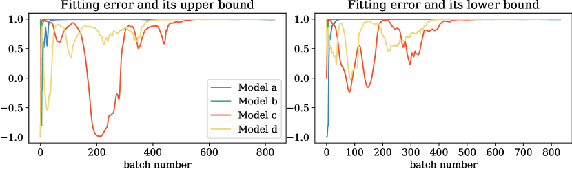
As shown in Figure 5, as training progresses, the variation in fitting error increasingly aligns with the trends of its upper and lower bounds. Concurrently, the gap between the bounds narrows. After the 500th epoch, the Pearson correlation coefficients between and its upper and lower bounds approach 1 across all models in Figure 5. These observations validate our proposed GSC algorithm and Theorem 4.7, demonstrating that minimizing the fitting error is effectively achieved by controlling its upper and lower bounds in model training.

We further analyze the changes in structural error and gradient norm during the training process, as illustrated in Figure 6. In Subsection 4.4, based on Theorem 4.5, the training process can be divided into two stages: the structural error optimization stage and the gradient norm control Stage. Specifically, during model training, structural error converges first, followed by a decrease in fitting error. This conclusion is fully consistent with the experimental results shown in Figure 6. Consequently, the PD learning framework, structural error and gradient norm optimization accurately describes the dynamics of model training.

6.3 Experimental result on the impact of model depth
In this subsection, we aim to analyze and validate the impact of model depth on learning performance. We first increase the depth of the models under the default initialization methods and observe changes in structural error. The results of this experiment are illustrated in Figure 7, leading to the following conclusions:
-
1.
Theorem 4.5 states that increasing the number of parameters reduces under the gradient independence condition, which is typically achieved through random parameter initialization. For Models a and d, which do not incorporate residual blocks, as the number of layers increases, rapidly decreases and approaches 1. This observation corroborates Theorem 4.5.
-
2.
The role of residual blocks in Model b and Model d has two aspects: one is to amplify the gradient values, and the other is that the presence of skip connections can invalidate the gradient independence condition. Therefore, according to Theorem 4.5, a model with residual blocks will have smaller and , as well as a larger . The experimental results for Model b and Model d, as shown in Figure 7, are consistent with the description provided by Theorem 4.5.


Next, we increment the value of from 0 to 5 in Models a and b and train these models to investigate the impact of model depth on training dynamics. The accuracy results of the models on the validation set are presented in 4.
| 0 | 1 | 2 | 3 | 4 | 5 | |
|---|---|---|---|---|---|---|
| Model a | 97.19% | 94.63% | 96.21% | 94.79% | 91.32% | 90.80% |
| Model b | 97.02% | 97.14% | 96.78% | 97.14% | 97.34% | 97.80% |
The experimental results concerning the impact of model depth on fitting error, and upper and lower bounds are illustrated in Figures 9 and 9. To examine the correlation between the fitting error and its bounds, we also computed the local Pearson correlation coefficients using a sliding window of length 50. The results are shown in Figures 11 and 11.


Below, we present the analysis of the experimental data and the conclusions drawn from it.
-
1.
In the absence of residual blocks, increasing model depth prolongs the time required for structural error to converge, thereby delaying the onset of fitting error reduction. As illustrated in Figure 9, as the number of layers increases, the timing at which the fitting error of Model a begins to decrease corresponds to the point when structural error converges. Increasing model depth prolongs the time required for structural error to converge, thereby delaying the onset of fitting error reduction. This observation aligns with Theorem 4.7, which implies that the optimization of fitting error depends on controlling its upper and lower bounds.
-
2.
In the absence of residual blocks, increasing model depth progressively fulfills the gradient independence condition. As illustrated in Figure 9, as the number of layers increases, , , and all approach zero, indicating that the structural error also tends toward zero. This phenomenon corroborates Theorem 4.5.
-
3.
Residual blocks disrupt the initial gradient independence condition but can accelerate the convergence of structural error. At the onset of training, even with an increase in the number of layers, Model b does not exhibit a reduction in structural error. We attribute this primarily to the fact that residual blocks disrupt the gradient independence condition. Consequently, Theorem 4.5 is no longer applicable. However, the presence of skip connections addresses the vanishing gradient problem associated with increased depth, allowing for the rapid establishment of a new gradient independence condition via SGD and thereby accelerating the convergence of structural error.
-
4.
Residual blocks mitigate or even eliminate the impact of increased depth on model convergence speed. As illustrated in Figures 11 and 11, the convergence rate of the correlation coefficients for Model b remains relatively stable despite increases in depth, demonstrating consistent convergence regardless of the number of layers.


To further analyze the mechanism by which residual blocks accelerate convergence, we compared the changes in gradient norm and structural error for Model a and Model b under different values of . These comparisons are illustrated in Figures 13 and 13. As illustrated in the figures, after convergence, both Model a and Model b exhibit a trend where the value of increases as the number of layers grows. However, when comparing Model a with Model b, it is evident that residual blocks mitigate the impact of layer count on , resulting in a smaller converged value of for Model b. Therefore, the incorporation of residual blocks significantly reduces when using deep models, thereby decreasing the gap between the upper and lower bounds of the fitting error and enhancing the stability of error convergence. This observation offers an evaluation perspective on the role of residual blocks from the standpoint of structural error.
7 Conclusion
This study introduces a novel theoretical learning framework, PD learning, which is characterized by its focus on the true underlying distribution. In order to learn the underlying distribution, we introduce the learning error as the optimization objective. To optimize the learning error, this paper proposes the necessary conditions for loss functions, models, and optimization algorithms. Based on these conditions, the non-convex optimization mechanism corresponding to model training can be theoretically resolved. We derive both model-independent and model-dependent upper bounds for the learning error, providing new insights into understanding machine learning. We illustrate that PD learning provides clearer insights into the unresolved issues in deep learning. The consistency of our framework with existing theories and experimental results, as well as the explanatory power of existing theories and phenomena, demonstrates the correctness and effectiveness of our proposed framework.
References
- [1] Moshe Leshno, V. Ya. Lin, Allan Pinkus, and Shimon Schocken. Original contribution: Multilayer feedforward networks with a nonpolynomial activation function can approximate any function. Neural Networks, 6:861–867, 1993.
- [2] Andrew R. Barron. Universal approximation bounds for superpositions of a sigmoidal function. IEEE Trans. Inf. Theory, 39:930–945, 1993.
- [3] Kenji Kawaguchi, Leslie Pack Kaelbling, and Yoshua Bengio. Generalization in deep learning. ArXiv, abs/1710.05468, 2017.
- [4] Yuhai Wu. Statistical learning theory. Technometrics, 41:377–378, 2021.
- [5] Peter L. Bartlett and Shahar Mendelson. Rademacher and gaussian complexities: Risk bounds and structural results. J. Mach. Learn. Res., 3:463–482, 2003.
- [6] Olivier Bousquet and André Elisseeff. Stability and generalization. Journal of Machine Learning Research, 2:499–526, 2002.
- [7] L. Oneto, Alessandro Ghio, Sandro Ridella, and D. Anguita. Fully empirical and data-dependent stability-based bounds. IEEE Transactions on Cybernetics, 45:1913–1926, 2015.
- [8] Andreas Maurer. A second-order look at stability and generalization. In Conference on learning theory, pages 1461–1475. PMLR, 2017.
- [9] André Elisseeff, Theodoros Evgeniou, and Massimiliano Pontil. Stability of randomized learning algorithms. J. Mach. Learn. Res., 6:55–79, 2005.
- [10] Sayan Mukherjee, Partha Niyogi, Tomaso A. Poggio, and Ryan M. Rifkin. Learning theory: stability is sufficient for generalization and necessary and sufficient for consistency of empirical risk minimization. Advances in Computational Mathematics, 25:161–193, 2006.
- [11] Shai Shalev-Shwartz, Ohad Shamir, Nathan Srebro, and Karthik Sridharan. Learnability, stability and uniform convergence. J. Mach. Learn. Res., 11:2635–2670, 2010.
- [12] Chiyuan Zhang, Samy Bengio, Moritz Hardt, Benjamin Recht, and Oriol Vinyals. Understanding deep learning requires rethinking generalization. ArXiv, abs/1611.03530, 2016.
- [13] Chiyuan Zhang, Samy Bengio, Moritz Hardt, Benjamin Recht, and Oriol Vinyals. Understanding deep learning (still) requires rethinking generalization. Communications of the ACM, 64:107 – 115, 2021.
- [14] Kaiming He, X. Zhang, Shaoqing Ren, and Jian Sun. Deep residual learning for image recognition. 2016 IEEE Conference on Computer Vision and Pattern Recognition (CVPR), pages 770–778, 2015.
- [15] Mikhail Belkin, Daniel J. Hsu, Siyuan Ma, and Soumik Mandal. Reconciling modern machine-learning practice and the classical bias–variance trade-off. Proceedings of the National Academy of Sciences, 116:15849 – 15854, 2018.
- [16] Vladimir N Vapnik and Y Alexey. Chervonenkis. on the uniform convergence of relative frequencies of events to their probabilities. Theory of Probability and its Applications, 16(2):264–280, 1971.
- [17] John Aldrich. R.a. fisher and the making of maximum likelihood 1912-1922. Statistical Science, 12:162–176, 1997.
- [18] Wolfgang Härdle, Marlene Müller, Stefan Sperlich, Axel Werwatz, et al. Nonparametric and semiparametric models, volume 1. Springer, 2004.
- [19] Geoffrey J McLachlan, Sharon X Lee, and Suren I Rathnayake. Finite mixture models. Annual review of statistics and its application, 6:355–378, 2019.
- [20] William Q Meeker, Luis A Escobar, and Francis G Pascual. Statistical methods for reliability data. John Wiley & Sons, 2022.
- [21] A. Ng and Michael I. Jordan. On discriminative vs. generative classifiers: A comparison of logistic regression and naive bayes. In Neural Information Processing Systems, 2001.
- [22] Julius Berner, Philipp Grohs, Gitta Kutyniok, and Philipp Christian Petersen. The modern mathematics of deep learning. ArXiv, abs/2105.04026, 2021.
- [23] Henry J. Kelley. Gradient theory of optimal flight paths. ARS Journal, 30:947–954, 1960.
- [24] Stuart E. Dreyfus. The numerical solution of variational problems. Journal of Mathematical Analysis and Applications, 5:30–45, 1962.
- [25] David E. Rumelhart, Geoffrey E. Hinton, and Ronald J. Williams. Learning representations by back-propagating errors. Nature, 323:533–536, 1986.
- [26] Andreas Griewank and Andrea Walther. Evaluating derivatives - principles and techniques of algorithmic differentiation, second edition. In Frontiers in applied mathematics, 2000.
- [27] Herbert E. Robbins. A stochastic approximation method. Annals of Mathematical Statistics, 22:400–407, 1951.
- [28] J. Kiefer and Jacob Wolfowitz. Stochastic estimation of the maximum of a regression function. Annals of Mathematical Statistics, 23:462–466, 1952.
- [29] Arkadi Nemirovski, Anatoli B. Juditsky, Guanghui Lan, and Alexander Shapiro. Robust stochastic approximation approach to stochastic programming. SIAM J. Optim., 19:1574–1609, 2008.
- [30] Rong Ge, Furong Huang, Chi Jin, and Yang Yuan. Escaping from saddle points - online stochastic gradient for tensor decomposition. ArXiv, abs/1503.02101, 2015.
- [31] J. Lee, Max Simchowitz, Michael I. Jordan, and Benjamin Recht. Gradient descent only converges to minimizers. In Annual Conference Computational Learning Theory, 2016.
- [32] Arnulf Jentzen, Benno Kuckuck, Ariel Neufeld, and Philippe von Wurstemberger. Strong error analysis for stochastic gradient descent optimization algorithms. Ima Journal of Numerical Analysis, 2018.
- [33] Grzegorz Lewicki and Giuseppe Marino. Approximation by superpositions of a sigmoidal function. Zeitschrift Fur Analysis Und Ihre Anwendungen, 22:463–470, 2003.
- [34] Ken ichi Funahashi. On the approximate realization of continuous mappings by neural networks. Neural Networks, 2:183–192, 1989.
- [35] Kurt Hornik, Maxwell B. Stinchcombe, and Halbert L. White. Multilayer feedforward networks are universal approximators. Neural Networks, 2:359–366, 1989.
- [36] Wassily Hoeffding. Probability inequalities for sums of bounded random variables. The collected works of Wassily Hoeffding, pages 409–426, 1994.
- [37] Leslie G Valiant. A theory of the learnable. Communications of the ACM, 27(11):1134–1142, 1984.
- [38] Huan Xu and Shie Mannor. Robustness and generalization. Machine Learning, 86:391 – 423, 2010.
- [39] Vaishnavh Nagarajan and J. Zico Kolter. Uniform convergence may be unable to explain generalization in deep learning. In Neural Information Processing Systems, 2019.
- [40] Mikhail Belkin, Alexander Rakhlin, and A. Tsybakov. Does data interpolation contradict statistical optimality? ArXiv, abs/1806.09471, 2018.
- [41] Mario Geiger, Arthur Jacot, Stefano Spigler, Franck Gabriel, Levent Sagun, Stéphane d’Ascoli, Giulio Biroli, Clément Hongler, and Matthieu Wyart. Scaling description of generalization with number of parameters in deep learning. Journal of Statistical Mechanics: Theory and Experiment, 2020, 2019.
- [42] Preetum Nakkiran, Gal Kaplun, Yamini Bansal, Tristan Yang, Boaz Barak, and Ilya Sutskever. Deep double descent: where bigger models and more data hurt. Journal of Statistical Mechanics: Theory and Experiment, 2021, 2019.
- [43] George V. Cybenko. Approximation by superpositions of a sigmoidal function. Mathematics of Control, Signals and Systems, 2:303–314, 1989.
- [44] Boris Hanin and Mark Sellke. Approximating continuous functions by relu nets of minimal width. ArXiv, abs/1710.11278, 2017.
- [45] Patrick Kidger and Terry Lyons. Universal approximation with deep narrow networks. ArXiv, abs/1905.08539, 2019.
- [46] Ben Poole, Subhaneil Lahiri, Maithra Raghu, Jascha Narain Sohl-Dickstein, and Surya Ganguli. Exponential expressivity in deep neural networks through transient chaos. In Neural Information Processing Systems, 2016.
- [47] Jingwei Zhang, Tongliang Liu, and Dacheng Tao. Going deeper, generalizing better: An information-theoretic view for deep learning. IEEE transactions on neural networks and learning systems, PP, 2023.
- [48] Yann Dauphin, Razvan Pascanu, Çaglar Gülçehre, Kyunghyun Cho, Surya Ganguli, and Yoshua Bengio. Identifying and attacking the saddle point problem in high-dimensional non-convex optimization. ArXiv, abs/1406.2572, 2014.
- [49] Simon Shaolei Du, Xiyu Zhai, Barnabás Póczos, and Aarti Singh. Gradient descent provably optimizes over-parameterized neural networks. ArXiv, abs/1810.02054, 2018.
- [50] Chulhee Yun, Suvrit Sra, and Ali Jadbabaie. Small nonlinearities in activation functions create bad local minima in neural networks. In International Conference on Learning Representations, 2018.
- [51] Lénaïc Chizat, Edouard Oyallon, and Francis R. Bach. On lazy training in differentiable programming. In Neural Information Processing Systems, 2018.
- [52] Yossi Arjevani and Michael Field. Annihilation of spurious minima in two-layer relu networks. ArXiv, abs/2210.06088, 2022.
- [53] Tomaso A. Poggio, Gil Kur, and Andy Banburski. Double descent in the condition number. ArXiv, abs/1912.06190, 2019.
- [54] Stéphane d’Ascoli, Levent Sagun, and Giulio Biroli. Triple descent and the two kinds of overfitting: where and why do they appear? Journal of Statistical Mechanics: Theory and Experiment, 2021, 2020.
- [55] Ben Adlam and Jeffrey Pennington. Understanding double descent requires a fine-grained bias-variance decomposition. ArXiv, abs/2011.03321, 2020.
- [56] Fanghui Liu, Johan A. K. Suykens, and Volkan Cevher. On the double descent of random features models trained with sgd. ArXiv, abs/2110.06910, 2021.
- [57] Sepp Hochreiter and Jürgen Schmidhuber. Flat minima. Neural Computation, 9:1–42, 1997.
- [58] Laurent Dinh, Razvan Pascanu, Samy Bengio, and Yoshua Bengio. Sharp minima can generalize for deep nets. In International Conference on Machine Learning, 2017.
- [59] Haowei He, Gao Huang, and Yang Yuan. Asymmetric valleys: Beyond sharp and flat local minima. In Neural Information Processing Systems, 2019.
- [60] Henning Petzka, Michael Kamp, Linara Adilova, Cristian Sminchisescu, and Mario Boley. Relative flatness and generalization. In Neural Information Processing Systems, 2020.
- [61] Jean Kaddour, Linqing Liu, Ricardo M. A. Silva, and Matt J. Kusner. When do flat minima optimizers work? In Neural Information Processing Systems, 2022.
- [62] Lei Wu, Ming Wang, and Weijie J. Su. The alignment property of sgd noise and how it helps select flat minima: A stability analysis. In Neural Information Processing Systems, 2022.
- [63] Frederic Koehler, Lijia Zhou, Danica J. Sutherland, and Nathan Srebro. Uniform convergence of interpolators: Gaussian width, norm bounds, and benign overfitting. In Neural Information Processing Systems, 2021.
- [64] Ke Wang, Vidya Muthukumar, and Christos Thrampoulidis. Benign overfitting in multiclass classification: All roads lead to interpolation. IEEE Transactions on Information Theory, 69:7909–7952, 2021.
- [65] Niladri S. Chatterji and Philip M. Long. Foolish crowds support benign overfitting. J. Mach. Learn. Res., 23:125:1–125:12, 2021.
- [66] Lisha Chen, Songtao Lu, and Tianyi Chen. Understanding benign overfitting in gradient-based meta learning. In Neural Information Processing Systems, 2022.
- [67] Vladimir Naumovich Vapnik. Estimation of dependences based on empirical data. Estimation of Dependences Based on Empirical Data, 2006.
- [68] L. Oneto. Model selection and error estimation in a nutshell. Modeling and Optimization in Science and Technologies, 2020.
- [69] Xijiong Xie and Shiliang Sun. Pac-bayes bounds for twin support vector machines. Neurocomputing, 234:137–143, 2017.
- [70] John Shawe-Taylor and Robert C. Williamson. A pac analysis of a bayesian estimator. In Annual Conference Computational Learning Theory, 1997.
- [71] David A. McAllester. Some pac-bayesian theorems. Machine Learning, 37:355–363, 1998.
- [72] David A. McAllester. Pac-bayesian model averaging. In Annual Conference Computational Learning Theory, 1999.
- [73] John Langford and Rich Caruana. (not) bounding the true error. In Neural Information Processing Systems, 2001.
- [74] Matthias W. Seeger. Pac-bayesian generalisation error bounds for gaussian process classification. J. Mach. Learn. Res., 3:233–269, 2003.
- [75] Andreas Maurer. A note on the pac bayesian theorem. ArXiv, cs.LG/0411099, 2004.
- [76] Ilya O. Tolstikhin and Yevgeny Seldin. Pac-bayes-empirical-bernstein inequality. In Neural Information Processing Systems, 2013.
- [77] Zakaria Mhammedi, Peter D. Grünwald, and Benjamin Guedj. Pac-bayes un-expected bernstein inequality. In Neural Information Processing Systems, 2019.
- [78] Omar Rivasplata, Ilja Kuzborskij, and Csaba Szepesvari. Pac-bayes analysis beyond the usual bounds. ArXiv, abs/2006.13057, 2020.
- [79] Pierre Alquier. User-friendly introduction to pac-bayes bounds. Found. Trends Mach. Learn., 17:174–303, 2021.
- [80] Léon Bottou, Frank E. Curtis, and Jorge Nocedal. Optimization methods for large-scale machine learning. ArXiv, abs/1606.04838, 2016.
- [81] Nitish Shirish Keskar, Dheevatsa Mudigere, Jorge Nocedal, Mikhail Smelyanskiy, and Ping Tak Peter Tang. On large-batch training for deep learning: Generalization gap and sharp minima. ArXiv, abs/1609.04836, 2016.
- [82] Pratik Chaudhari and Stefano Soatto. Stochastic gradient descent performs variational inference, converges to limit cycles for deep networks. 2018 Information Theory and Applications Workshop (ITA), pages 1–10, 2017.
- [83] J. Lee, Ioannis Panageas, Georgios Piliouras, Max Simchowitz, Michael I. Jordan, and Benjamin Recht. First-order methods almost always avoid strict saddle points. Mathematical Programming, 176:311 – 337, 2019.
- [84] Stanislaw Jastrzebski, Zachary Kenton, Devansh Arpit, Nicolas Ballas, Asja Fischer, Yoshua Bengio, and Amos J. Storkey. Three factors influencing minima in sgd. ArXiv, abs/1711.04623, 2017.
- [85] Aitor Lewkowycz, Yasaman Bahri, Ethan Dyer, Jascha Narain Sohl-Dickstein, and Guy Gur-Ari. The large learning rate phase of deep learning: the catapult mechanism. ArXiv, abs/2003.02218, 2020.
- [86] Radford M Neal and Radford M Neal. Priors for infinite networks. Bayesian learning for neural networks, pages 29–53, 1996.
- [87] Christopher K. I. Williams. Computing with infinite networks. In Neural Information Processing Systems, 1996.
- [88] Ole Winther. Computing with finite and infinite networks. In Neural Information Processing Systems, 2000.
- [89] Radford M Neal. Bayesian learning for neural networks, volume 118. Springer Science & Business Media, 2012.
- [90] Jaehoon Lee, Yasaman Bahri, Roman Novak, Samuel S. Schoenholz, Jeffrey Pennington, and Jascha Narain Sohl-Dickstein. Deep neural networks as gaussian processes. ArXiv, abs/1711.00165, 2017.
- [91] Arthur Jacot, Franck Gabriel, and Clément Hongler. Neural tangent kernel: Convergence and generalization in neural networks. ArXiv, abs/1806.07572, 2018.
- [92] Yuanzhi Li and Yingyu Liang. Learning overparameterized neural networks via stochastic gradient descent on structured data. ArXiv, abs/1808.01204, 2018.
- [93] Sanjeev Arora, Simon Shaolei Du, Wei Hu, Zhiyuan Li, and Ruosong Wang. Fine-grained analysis of optimization and generalization for overparameterized two-layer neural networks. ArXiv, abs/1901.08584, 2019.
- [94] Simon Shaolei Du, J. Lee, Haochuan Li, Liwei Wang, and Xiyu Zhai. Gradient descent finds global minima of deep neural networks. ArXiv, abs/1811.03804, 2018.
- [95] Zeyuan Allen-Zhu, Yuanzhi Li, and Yingyu Liang. Learning and generalization in overparameterized neural networks, going beyond two layers. In Neural Information Processing Systems, 2018.
- [96] Difan Zou, Yuan Cao, Dongruo Zhou, and Quanquan Gu. Stochastic gradient descent optimizes over-parameterized deep relu networks. ArXiv, abs/1811.08888, 2018.
- [97] Zeyuan Allen-Zhu, Yuanzhi Li, and Zhao Song. A convergence theory for deep learning via over-parameterization. ArXiv, abs/1811.03962, 2018.
- [98] Justin A. Sirignano and Konstantinos V. Spiliopoulos. Mean field analysis of neural networks: A central limit theorem. Stochastic Processes and their Applications, 2018.
- [99] Song Mei, Andrea Montanari, and Phan-Minh Nguyen. A mean field view of the landscape of two-layer neural networks. Proceedings of the National Academy of Sciences of the United States of America, 115:E7665 – E7671, 2018.
- [100] Lénaïc Chizat and Francis R. Bach. On the global convergence of gradient descent for over-parameterized models using optimal transport. ArXiv, abs/1805.09545, 2018.
- [101] Jeffrey Negrea, Mahdi Haghifam, Gintare Karolina Dziugaite, Ashish Khisti, and Daniel M. Roy. Information-theoretic generalization bounds for sgld via data-dependent estimates. ArXiv, abs/1911.02151, 2019.
- [102] Fredrik Hellström and Giuseppe Durisi. A new family of generalization bounds using samplewise evaluated cmi. ArXiv, abs/2210.06422, 2022.
- [103] Aolin Xu and Maxim Raginsky. Information-theoretic analysis of generalization capability of learning algorithms. ArXiv, abs/1705.07809, 2017.
- [104] Amir-Reza Asadi, Emmanuel Abbe, and Sergio Verdú. Chaining mutual information and tightening generalization bounds. ArXiv, abs/1806.03803, 2018.
- [105] Ruida Zhou, Chao Tian, and Tie Liu. Stochastic chaining and strengthened information-theoretic generalization bounds. 2022 IEEE International Symposium on Information Theory (ISIT), pages 690–695, 2022.
- [106] Eugenio Clerico, Amitis Shidani, George Deligiannidis, and A. Doucet. Chained generalisation bounds. In Annual Conference Computational Learning Theory, 2022.
- [107] Yuheng Bu, Shaofeng Zou, and Venugopal V. Veeravalli. Tightening mutual information based bounds on generalization error. 2019 IEEE International Symposium on Information Theory (ISIT), pages 587–591, 2019.
- [108] Mahdi Haghifam, Jeffrey Negrea, Ashish Khisti, Daniel M. Roy, and Gintare Karolina Dziugaite. Sharpened generalization bounds based on conditional mutual information and an application to noisy, iterative algorithms. ArXiv, abs/2004.12983, 2020.
- [109] Borja Rodr’iguez G’alvez, Germán Bassi, Ragnar Thobaben, and Mikael Skoglund. Tighter expected generalization error bounds via wasserstein distance. In Neural Information Processing Systems, 2021.
- [110] Ruida Zhou, Chao Tian, and Tie Liu. Individually conditional individual mutual information bound on generalization error. 2021 IEEE International Symposium on Information Theory (ISIT), pages 670–675, 2020.
- [111] Ravid Shwartz-Ziv and Naftali Tishby. Opening the black box of deep neural networks via information. ArXiv, abs/1703.00810, 2017.
- [112] Kartik Ahuja, Ethan Caballero, Dinghuai Zhang, Yoshua Bengio, Ioannis Mitliagkas, and Irina Rish. Invariance principle meets information bottleneck for out-of-distribution generalization. In Neural Information Processing Systems, 2021.
- [113] Shelvia Wongso, Rohan Ghosh, and M. Motani. Using sliced mutual information to study memorization and generalization in deep neural networks. In International Conference on Artificial Intelligence and Statistics, 2023.
- [114] Fredrik Hellström and Giuseppe Durisi. Evaluated cmi bounds for meta learning: Tightness and expressiveness. ArXiv, abs/2210.06511, 2022.
- [115] Haiyun He, Hanshu Yan, and Vincent Y. F. Tan. Information-theoretic characterization of the generalization error for iterative semi-supervised learning. J. Mach. Learn. Res., 23:287:1–287:52, 2021.
- [116] Xuetong Wu, Jonathan H. Manton, Uwe Aickelin, and Jingge Zhu. Information-theoretic analysis for transfer learning. 2020 IEEE International Symposium on Information Theory (ISIT), pages 2819–2824, 2020.
- [117] L. Oneto, Sandro Ridella, and D. Anguita. Do we really need a new theory to understand over-parameterization? Neurocomputing, 543:126227, 2023.
- [118] SM Mahbubur Rahman, M Omair Ahmad, and MNS Swamy. Bayesian wavelet-based image denoising using the gauss–hermite expansion. IEEE Transactions on Image Processing, 17(10):1755–1771, 2008.
- [119] Herbert A Sturges. The choice of a class interval. Journal of the american statistical association, 21(153):65–66, 1926.
- [120] David W Scott. On optimal and data-based histograms. Biometrika, 66(3):605–610, 1979.
- [121] David Freedman and Persi Diaconis. On the histogram as a density estimator: L 2 theory. Zeitschrift für Wahrscheinlichkeitstheorie und verwandte Gebiete, 57(4):453–476, 1981.
- [122] Emanuel Parzen. On estimation of a probability density function and mode. The annals of mathematical statistics, 33(3):1065–1076, 1962.
- [123] Bernard W Silverman. Density estimation for statistics and data analysis. Routledge, 2018.
- [124] Peter Hall, Jeff Racine, and Qi Li. Cross-validation and the estimation of conditional probability densities. Journal of the American Statistical Association, 99(468):1015–1026, 2004.
- [125] Anders Hald. On the history of maximum likelihood in relation to inverse probability and least squares. Statistical Science, 14:214–222, 1999.
- [126] Peter J. Huber. Robust estimation of a location parameter. Annals of Mathematical Statistics, 35:492–518, 1964.
- [127] Peter J. Huber. Robust regression: Asymptotics, conjectures and monte carlo. Annals of Statistics, 1:799–821, 1973.
- [128] David JC MacKay. Information theory, inference and learning algorithms. Cambridge university press, 2003.
- [129] Devinderjit Sivia and John Skilling. Data analysis: a Bayesian tutorial. OUP Oxford, 2006.
- [130] Kevin P Murphy. Probabilistic machine learning: an introduction. MIT press, 2022.
- [131] Hugo Larochelle and Iain Murray. The neural autoregressive distribution estimator. In Proceedings of the fourteenth international conference on artificial intelligence and statistics, pages 29–37. JMLR Workshop and Conference Proceedings, 2011.
- [132] George Papamakarios, Theo Pavlakou, and Iain Murray. Masked autoregressive flow for density estimation. Advances in neural information processing systems, 30, 2017.
- [133] Danilo Rezende and Shakir Mohamed. Variational inference with normalizing flows. In International conference on machine learning, pages 1530–1538. PMLR, 2015.
- [134] Laurent Dinh, Jascha Sohl-Dickstein, and Samy Bengio. Density estimation using real nvp. arXiv preprint arXiv:1605.08803, 2016.
- [135] Jiajin Li, Anthony Man-Cho So, and Wing-Kin Ma. Understanding notions of stationarity in nonsmooth optimization: A guided tour of various constructions of subdifferential for nonsmooth functions. IEEE Signal Processing Magazine, 37:18–31, 2020.
- [136] Mathieu Blondel, André F. T. Martins, and Vlad Niculae. Learning with fenchel-young losses. ArXiv, abs/1901.02324, 2019.
- [137] Thomas M Cover. Elements of information theory. John Wiley & Sons, 1999.
- [138] Paul Dupuis and Richard S Ellis. A weak convergence approach to the theory of large deviations. John Wiley & Sons, 2011.
- [139] Avrim Blum, John Hopcroft, and Ravindran Kannan. Foundations of data science. Cambridge University Press, 2020.
- [140] T. M. Cover. Elements of Information Theory (Wiley Series in Telecommunications and Signal Processing). Elements of Information Theory (Wiley Series in Telecommunications and Signal Processing), 2017.
- [141] Christian Szegedy, Vincent Vanhoucke, Sergey Ioffe, Jonathon Shlens, and Zbigniew Wojna. Rethinking the inception architecture for computer vision. 2016 IEEE Conference on Computer Vision and Pattern Recognition (CVPR), pages 2818–2826, 2015.
- [142] N. Chawla, K. Bowyer, Lawrence O. Hall, and W. Philip Kegelmeyer. Smote: Synthetic minority over-sampling technique. ArXiv, abs/1106.1813, 2002.
- [143] Xavier Glorot and Yoshua Bengio. Understanding the difficulty of training deep feedforward neural networks. In International Conference on Artificial Intelligence and Statistics, 2010.
- [144] Kaiming He, X. Zhang, Shaoqing Ren, and Jian Sun. Delving deep into rectifiers: Surpassing human-level performance on imagenet classification. 2015 IEEE International Conference on Computer Vision (ICCV), pages 1026–1034, 2015.
- [145] David Balduzzi, Marcus Frean, Lennox Leary, J. P. Lewis, Kurt Wan-Duo Ma, and Brian McWilliams. The shattered gradients problem: If resnets are the answer, then what is the question? ArXiv, abs/1702.08591, 2017.
- [146] Alex Krizhevsky, Ilya Sutskever, and Geoffrey E. Hinton. Imagenet classification with deep convolutional neural networks. Communications of the ACM, 60:84 – 90, 2012.
- [147] Yann LeCun, Léon Bottou, Yoshua Bengio, and Patrick Haffner. Gradient-based learning applied to document recognition. Proc. IEEE, 86:2278–2324, 1998.
Appendix A Appendix
In this section, we prove the results stated in the paper and provide necessary technical details and discussions.
A.1 Proof of Theorem 4.2
Assuming , the frequency distribution , inferred from the sample , adheres to a multinomial distribution: . With the provision of i.i.d. sample data and a prior distribution such that , the application of Bayes’s theorem facilitates the derivation of the posterior distribution for .
| (28) | ||||
where .
A.2 Proof of Theorem 4.3
Since is continuous, differentiable, and has a unique minimum value of zero at , where its gradient with respect to vanishes, i.e., , we can express this gradient as
| (29) |
Due to the uniqueness of the minimum value, the expected loss, , is strictly convex, and at its minimum , where , the gradient with respect to vanishes, i.e., , which implies that , where .
Given that is an arbitrary distribution function, must be independent of , allowing us to replace with . Since is a strictly convex function, its Hessian with respect to can be derived as:
| (30) |
Simplifying we get:
| (31) |
The inequality above is derived from the fact that is strictly convex.
When is set to , we have . Since can take any value, it follows that for any arbitrary , we get .
Let us define a strictly convex function with its Hessian matrix given by . The gradient of the loss function with respect to can be expressed as follows:
| (32) | ||||
Since , we find that , where is a constant. This leads to the following expression for the loss function:
| (33) | ||||
A.3 Proof of Theorem 4.5
Since each column of is uniformly from the ball , according to Theorem 3.4, then with probability the following holds:
| (34) | ||||
Because is a symmetric positive semidefinite matrix, then we have . Then the following holds with probability at least
| (35) | |||
Since and , then we have
| (38) | ||||
By dividing both sides of the aforementioned inequality by the corresponding sides of inequalities (35), we obtain:
| (39) |
where .
A.4 Proof of Theorem 4.4
According to the given definition, we have
| (40) |
where , . Let denote the eigenvalue decomposition of . Consequently, is a diagonal matrix whose entries are the eigenvalues of . We then have
| (41) | ||||
where . The final step is equivalent to
| (42) |
Similarly, we obtain
| (43) |
It follows that
| (44) |
A.5 Proof of Theorem 4.6
According to the Bayesian theorem and Sanov’s theorem 3.2, we have
| (45) | ||||
Therefore, we obtain
| (46) |
Since is finite, we have
| (47) |
Since and are both unbiased and consistent estimators of , it follows that
| (48) | ||||
A.6 Proof of Theorem 4.7
Utilizing the triangle inequality of norms, we obtain
| (49) |
Substituting the above inequality into equalities 13 completes the proof.
A.7 Proof of Theorem 4.8
Let be a vector of dimension . According to the definition of the norm, we have
| (50) | ||||
Consequently, we obtain
| (51) | ||||
where the last inequality is based on Pinsker’s inequality 3.6. Since there exists such that , it follows that
| (52) | ||||
where .
A.8 Proof of Theorem 5.1
Since represents the minimum point of , where , it follows that :
| (53) | |||
By applying the mean value theorem, there exists such that the following inequalities hold:
| (54) | ||||
where the first inequality is based on the Cauchy-Schwarz inequality, and the second inequality follows from the definition of the matrix-induced 2-norm. Consequently, within the neighborhood of , that is , we have
| (55) |
where . That is, there exists such that
| (56) |
It indicates that and are equivalent. Therefore, is equivalent to minimizing . Given the equation:
and since is model-independent, it follows that is equivalent to
where .
Appendix B Declarations
B.1 Funding
This work was supported in part by the National Key Research and Development Program of China under No. 2022YFA1004700, Shanghai Municipal Science and Technology, China Major Project under grant 2021SHZDZX0100, the National Natural Science Foundation of China under Grant Nos. 62403360, 72171172, 92367101, 62088101, iF open-funds from Xinghuo Eco and China Institute of Communications.
B.2 Competing interests
The authors declare that they have no known competing financial interests or personal relationships that could have appeared to influence the work reported in this paper.
B.3 Ethics approval and consent to participate
Not applicable.
B.4 Data availability
B.5 Materials availability
Not applicable.
B.6 Code availability
Code for preprocessing and analysis is provided in the GitHub repository pd_learning.
B.7 Author contribution
Binchuan Qi: Conceptualization, Methodology, Writing original draft. Wei Gong: Supervision, Review, Declarations. Li Li: Supervision, Review, Declarations.