Probabilistic Traversability Model for Risk-Aware Motion Planning in Off-Road Environments
Abstract
A key challenge in off-road navigation is that even visually similar terrains or ones from the same semantic class may have substantially different traction properties. Existing work typically assumes no wheel slip or uses the expected traction for motion planning, where the predicted trajectories provide a poor indication of the actual performance if the terrain traction has high uncertainty. In contrast, this work proposes to analyze terrain traversability with the empirical distribution of traction parameters in unicycle dynamics, which can be learned by a neural network in a self-supervised fashion. The probabilistic traction model leads to two risk-aware cost formulations that account for the worst-case expected cost and traction. To help the learned model generalize to unseen environment, terrains with features that lead to unreliable predictions are detected via a density estimator fit to the trained network’s latent space and avoided via auxiliary penalties during planning. Simulation results demonstrate that the proposed approach outperforms existing work that assumes no slip or uses the expected traction in both navigation success rate and completion time. Furthermore, avoiding terrains with low density-based confidence score achieves up to 30% improvement in success rate when the learned traction model is used in a novel environment.
Supplementary Material
Video and GPU implementation of planners are available at https://github.com/mit-acl/mppi_numba.
I Introduction
Progress in autonomous robot navigation has expanded the set of non-urban environments where robots can be deployed, such as mines, forests, oceans and Mars [1, 2, 3, 4]. Unlike environments where safe and reliable navigation can be achieved by avoiding hazards easily detected based on geometric features, navigation in forested environments poses unique challenges that still prevent systems from achieving good performance, because a purely geometric view of the world is not sufficient to identify non-geometric hazards (e.g., mud puddles, slippery surfaces) and geometric non-hazards (e.g., grass and foliage). To this end, recent approaches train semantic classifiers for camera images [5, 6, 7, 8, 9] or lidar pointclouds [10] to identify terrains or objects that could cause failures to the robotic platform in order to manually design semantics-based cost functions for navigation. However, existing labeled datasets for off-road navigation have limited number of class labels such as “bush”, “grass”, and “tree” for vegetation without capturing the varying traversability within each class (e.g., [11, 12]), or have limited transferability due to specificity to the vehicles that collected the data.
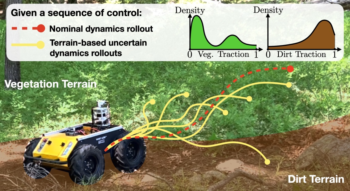
While manually designing cost functions based on semantically labeled terrains are common, self-supervised learning techniques are increasingly adopted to model traversability based on historically collected data about terrain properties [13, 14, 15]. For example, a robot can learn to map camera images to terrain properties such as traction that affects achievable velocities [16, 17, 18]. However, these methods do not fully account for the uncertainty in the learned terrain models. Based on our empirical findings (see the real-world traction distribution learned by a neural network (NN) in the “Traversability Analysis” block of Fig. 3), terrains properties such as traction can be non-Gaussian, which makes assuming no slip or using the expected traction inadequate to capture the risk of obtaining poor performance. Even if the full empirical distribution can be learned about the traction parameters, working with distributions that are not necessarily Gaussian makes it difficult to efficiently characterise and estimate the cost of experiencing tail events during planning.
In this work, we propose to analyze terrain traversability with the empirical distribution of traction parameters in the unicycle model without making Gaussian assumptions. In addition, we propose two cost formulations that exploit the learned traction distribution to estimate the impact of tail events on navigation performance. The resultant planners mitigate the risks that stem from the stochastic dynamics and the downstream realization of the objectives. Lastly, as a NN’s predictions are unreliable when input features are significantly different from training data, we fit a Gaussian Mixture Model (GMM) in the latent space of the trained NN to provide confidence scores for detecting and avoiding novel terrains via auxiliary planning costs. In summary, the contributions of this work are:
-
•
A new representation of traversability as an empirical traction distribution in the unicycle dynamics conditioned on both semantic and geometric terrain features;
-
•
Two risk-aware cost formulations based on the worst-case expected traction and objective that outperform methods that assume no slip or use expected traction;
-
•
A GMM-based detector for detecting terrains that may lead to unreliable NN predictions and should be avoided during planning, which improves navigation success rate by 30% when a learned traction model is used in an environment unseen during training.
II Related Work
II-A Traversability Representation
Traversability analysis is a key component of off-road navigation algorithms; a more complete summary of various approaches is provided in [17], including representations based on proprioceptive measurements [19, 20], geometric features [21, 22, 23, 1] and combination of geometric and semantic features [24, 25, 10]. WayFast [16] is a more recent approach, similar to this work, that proposes to represent traversability by learning traction coefficients for a unicycle model from terrain perception data. Another recent work [2] represents traversability as the probability of a quadruped robot to stabilize itself on uneven terrain, based on 3D occupancy data of the terrain. In [26], speed and gait policies are learned based on terrain semantics and human demonstrations; these policies provide a novel interpretation of the terrain’s traversability and can be used by the robot’s motor control policy. A key limitation, however, is that these point estimates of traversability do not capture the uncertainty of terrain properties on similar-looking terrains. Instead, our approach represents traversability as the distribution of traction parameters in the dynamics model.
II-B Planning with Terrain-Dependent Stochastic Dynamics
After learning the traction distribution in the dynamics model, a further challenge exists in incorporating this model into the planner. Despite capturing various types of uncertainties and risks, many existing methods still plan with the nominal or expected parameters in the dynamics model, such as [25, 27, 17]. Alternatively, our work is inspired by [28] that proposes a general framework for optimizing the conditional value at risk (CVaR) of the objective under uncertain dynamics, parameters and initial conditions, by taking extra samples from sources of uncertainty. In this work, we evaluate each control sequence based on traction samples and use the CVaR of the noisy realizations of the objectives instead of the nominal objective. Additionally, we propose a more computationally efficient approach which computes the nominal objective using trajectory rollouts based on the CVaR of traction parameters. Compared to WayFast [16] that uses the expected traction values (a risk-neutral special case of our second method), our approach can produce behaviors that are more risk-averse by adjusting the worst-case quantiles used to compute the CVaR of traction.
II-C Uncertainty Estimation for Neural Networks
Data collection in practice is often expensive and limited in diversity, so it is important to know when a learned model cannot be trusted (e.g., due to input features that are significantly different from training data). NN uncertainty estimation is well studied in the machine learning literature (e.g., see survey [29]), where representative techniques include Monte Carlo dropouts [30], ensembles [31], and single-pass methods [32]. Most similar to the single-pass technique [32] that only requires a single neural network evaluation to estimate uncertainty, our work tries to capture the aleatoric uncertainty (the inherent process uncertainty that cannot be reduced with more data) by predicting a distribution, and the epistemic uncertainty (the model uncertainty that can be reduced with more data) by leveraging the latent space density of NN. Compared to using dropouts or ensembles, single-pass methods are attractive, because they do not require taking extra samples or using more memory.
III Problem Formulation
We consider the problem of motion planning for a wheeled vehicle whose dynamics depend on the underlying terrains, where the traction values are uncertain due to imperfect sensing. Therefore, we model traction values as random variables whose distributions can be learned empirically.
III-A Unicycle Model with Uncertain Traction Parameters
Consider the discrete time system:
| (1) |
where is the state vector, is the control input, and is the parameter vector that captures the terrain traction. For each mission, terrain-dependent parameter vectors are sampled from the ground truth distribution for every and the associated terrain features . For concreteness, we use the following unicycle model
| (2) |
where contains the X, Y positions and yaw, contains the linear and angular velocities, contains the linear and angular traction values , and is the time interval. Intuitively, traction captures how much of the commanded velocities can be achieved and is a good indicator for terrain traversability for fast off-road navigation.
III-B Motion Planning
As this work focuses on achieving fast navigation to a given goal position, we adopt and modify the minimum-time formulation used in [17], but any other task-specific objectives can be used instead. Given initial state and goal position , the problem of finding a sequence of control can be written as
| (3) | ||||
| s.t. | (4) |
where and are the terminal cost and the stage cost:
| (5) | ||||
| (6) |
where is the default speed for estimating time-to-go at the end of the rollout, is the sampling duration, is the robot position at , and is the weight for penalizing distance from the goal. To avoid accumulating costs after robot reaches the goal, we use an indicator function that returns when any state has reached for , and returns otherwise. Intuitively, the objective encourages the robot to arrive at the goal location as quickly as possible.
While the problem (3) can be optimized via non-linear optimization techniques such as Model Predictive Path Integral control (MPPI [33, Algorithm 2]), the main challenge is that the terrain traction is uncertain. To address this issue, existing techniques try to learn the expected traction, or use nominal traction while penalizing undesirable terrains manually. However, these approaches are either risk-neutral or require human expertise in cost design. In this work, we propose to learn the full traction distribution empirically (Sec. IV) that can be used to design risk-aware costs with easy-to-tune risk tolerance (Sec. V).
IV Traversability Model
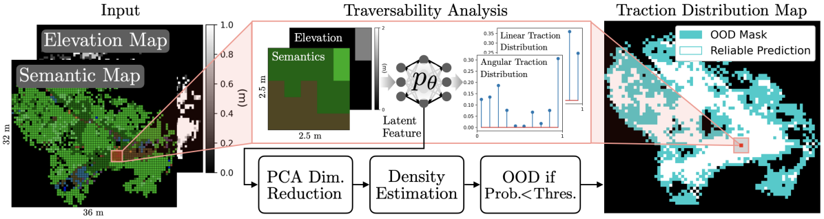
In this section, we introduce how to learn traction distribution (aleatoric uncertainty) and how to leverage density estimation in the trained NN’s latent space for detecting unfamiliar terrains (epistemic uncertainty). An overview of the entire traversability analysis procedure is shown in Fig. 3.
IV-A Terrain-Dependent Traction Distribution
Given the set of system parameters and the set of terrain features , we want to model the conditional distribution
| (7) |
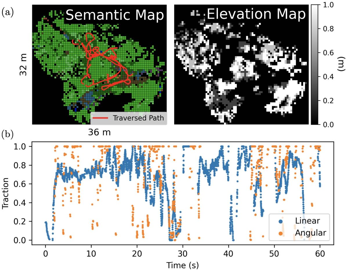
where is a probability distribution parameterized by , which in practice can be learned by a NN using empirically collected dataset where . A real world example can be found in Fig. 2 where a Clearpath Husky was manually driven in a forest to build an environment model and collect traction data. Note that the semantic and geometric information about the environment can be built by using a semantic octomap [34] that temporally fuses semantic point clouds. We used PointRend [35] trained on RUGD off-road navigation dataset [11] to segment RGB images and subsequently projected the semantics onto lidar point clouds. To estimate the true linear and angular velocities of the robot, we could not rely on the wheel-encoders due to wheel slips. Therefore, we used direct lidar odometry [36] that produced accurate pose estimates even when driving through tall grass, and the resultant pose estimates were fused with IMU measurements in an extended Kalman filter to obtain the high-rate velocity estimates. The velocity estimates were further filtered to reduce noise due to bumpy terrains. Finally, the traction values were computed as the ratios between the estimated and the commanded velocities and stored for offline training.
Given terrain features, traversed path and estimated traction values, we can train a NN (e.g., with convolutional layers followed by fully connected layers) to map local terrain features to categorical distributions over discretized traction values in order to capture rich terrain properties. To facilitate planning, we store learned traction distributions in a map , where each cell indexed by row and height stores the traction distribution that has already been conditioned on the associated terrain features.
IV-B Density-Based Detector for Unfamiliar Terrain Features
As the learned traction predictor is trained on limited data, its predictions based on terrain features significantly different from training data are unreliable, which can lead to degraded navigation performance. Therefore, we fit a density estimator in the latent space of the trained NN in order to use the predicted likelihood as a measure of model uncertainty.
We first apply principal component analysis (PCA) to the latent space features that correspond to all the terrain features observed during training . Next, we fit a Gaussian Mixture Model (GMM) for the entire training dataset in the reduced latent space, where the likelihood of observing a particular feature is denoted as . We design a simple confidence score based on the log-likelihood of the query data normalized between the maximum and minimum log-likelihood observed in training data:
| (8) | ||||
| (9) | ||||
| (10) |
Note that is not limited to and lower values indicate that the terrain features are less similar to the training data. With the NN trained in the environment shown in Fig. 2, we project the latent space features to the first 2 principle components and fit a GMM with 2 clusters. During deployment, terrain features with confidence score below some threshold are deemed out-of-distribution (OOD) and the OOD terrains should be explicitly avoided during planning via auxiliary penalties. This strategy improves navigation success rate when the NN is deployed in an environment unseen during training (see Sec. VI-C).
V Planning with Learned Traction Distribution
Given the learned traction model, we propose two risk-aware cost formulations in order to generate control input that is less likely to lead to worst-case failures. Note that the proposed cost formulations can substitute the nominal objective in (3) and the problem can still be solved normally using nonlinear optimization technique such as MPPI.
V-A Conditional Value at Risk (CVaR)
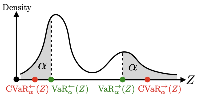
We adopt the Conditional Value at Risk (CVaR) as a risk metric because it satisfies a group of axioms important for rational risk assessment [37], but the conventional definition assumes the worst-case occurs at the right tail of the distribution. In this work, we define CVaR at both the right and left tails (see Fig. 5) at level for the random variable and its possible realization as follows:
| (11) | ||||
| (12) |
where the right and left Values at Risk are defined as:
| (13) | ||||
| (14) |
Intuitively, and capture the expected outcomes that fall in the right tail and left tail of the distribution, respectively, where each tail occupies portion of the total probability. Notice that either definition of CVaR produces the mean when .
V-B Risk-Aware Cost Formulations
In order to account for the risk of obtaining high cost due to the uncertain system parameters , we propose to optimize two modified versions of the cost function (3). Fig. 5 gives a high-level illustration of the core ideas behind the two cost functions.
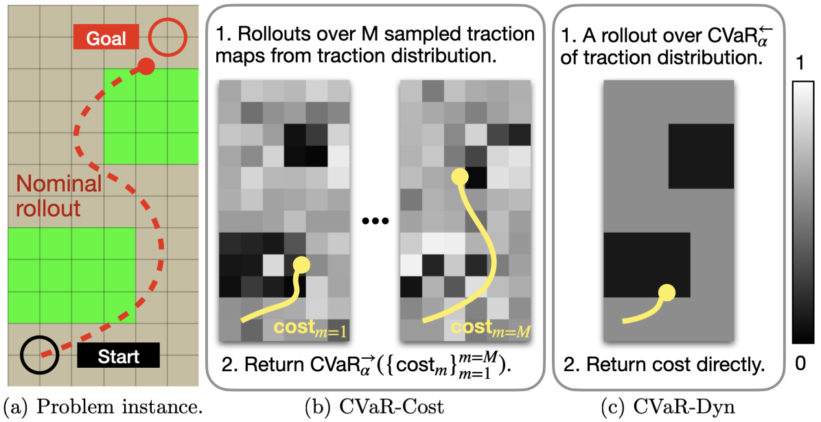
V-B1 Worst-Case Expected Cost (CVaR-Cost)
Given the control sequence , we want to evaluate the worst-case expected value for the nominal objective (3) due to uncertain terrain traction. First, we sample from the traction distribution map to obtain traction maps that contain samples of traction values from distribution in every map cell indexed by height and width for each sample index . Next, we compute the empirical right-tail CVaR of the performances of the rollouts:
| (15) |
where the -th state rollout follows
| (16) |
for . The traction parameter is queried in the -th sampled traction map at state . Note that this approach is inspired by [28], but we additionally handle terrain-dependent distributions of parameters and the sampling of traction maps. For better real-time performance, the sampled traction maps can be reused for evaluating different control sequences.
V-B2 Worst-Case Expected System Parameters (CVaR-Dyn)
The procedure for evaluating a control sequence over a large number of sampled traction maps can be efficiently parallelized on GPUs, but the computational overhead can still grow prohibitively when considering many control sequences. Therefore, we propose an alternative cost design that accounts for the worst-case expectation of the traction values in the dynamical model.
Given the control sequence , we evaluate the nominal mission objective (3) based on the state rollout simulated with the worst-case expected traction, i.e.,
| (17) |
where the state rollout follows
| (18) |
for and the worst-case expected traction is computed based on the corresponding traction distribution at some row and height determined by state :
| (19) |
When , the expected values of the traction parameters are used, equivalent to the approach in [16]. However, as the results in Sec. VI-B show for a go-to-goal task, planning with the worst-case expected traction can improve navigation performance when the traction distribution is not Gaussian.
Remark 1.
Remark 2.
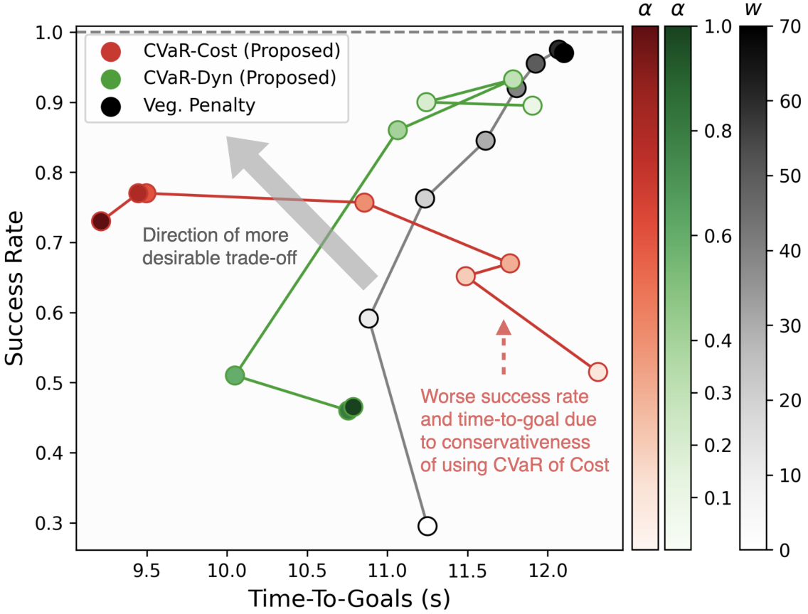
While adding auxiliary penalties for trajectories entering low-traction terrains can generate similar risk-aware behaviors achievable by our approach, we show that using the proposed costs (15) and (17) leads to solutions with better trade-offs between success rate and time-to-goal than ones achieved by using the nominal objective augmented with terrain penalties (see Fig. 8). However, the highest success rate achieved by using the proposed cost formulations are lower. Combining the best of both worlds, using the proposed costs with auxiliary penalties for undesirable terrains, such as OOD terrains, lead to better performance (see Sec. VI-C).
VI Simulation Results
Using simulated semantic environments, we show that the proposed methods outperform existing approaches [16, 17] that either assume no slip or use expected traction. Moreover, we discuss the advantages and limitations of our proposed risk-aware costs compared to auxiliary penalties for low-traction terrains. Lastly via simulations based on real-world traction data, we show that avoiding OOD terrains improves navigation success rate, and using our approach with auxiliary cost for OOD terrains improves time-to-goals. To prevent simulations from running indefinitely when the robot encounters near-zero traction, we impose time limits (selected based on mission difficulties) that are much longer than the average time required to complete the missions.
VI-A Implementation Details
In order to solve the optimization problem (3), we adopt MPPI [33, Algorithm 2] to generate control for achieving fast navigation to goal. This approach is attractive because it is derivative-free, parallelizable on GPU, and works with our proposed risk-aware cost formulations (15) and (17). The MPPI planners run in a receding horizon fashion with 100 time steps and each step is 0.1 s. The max linear and angular speeds are capped at 3 m/s and rad/s, and the noise standard deviations for the control signals are 2 m/s and 2 rad/s. The number of control rollouts is 1024 and the number of sampled traction maps is 1024 (only applicable for the CVaR-Cost). We use probability mass functions with 20 uniform bins to approximate the parameter distribution. The CVaR-Cost planner is the most expensive to compute, but it is able to re-plan at 15 Hz while sampling new control actions and maps with dimension of . Planners that do not sample traction maps can be executed at over 50 Hz. A computer with Intel Core i9 CPU and Nvidia GeForce RTX 3070 GPU is used for the simulations, where majority of the computation happens on the GPU.
VI-B Simulated Semantic Environments
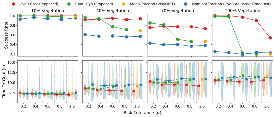
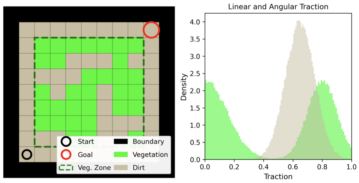
We consider a grid world scenario where “dirt” and “vegetation” cells have known traction distributions, as shown in Fig. 7. Vegetation patches are randomly spawned with increasing probabilities at the center of the arena, and a robot may experience significant slow-down for certain vegetation cells due to vegetation’s bi-modal distribution. The mission is deemed successful if the goal is reached within 15 s.
Overall, we sample different semantic maps and random realizations of traction parameters for every semantic map. The traction parameters are drawn before starting each trial and remain fixed. The benchmark results can be found in Fig. 6, where we compare the two proposed costs with existing methods, namely WayFAST [16] that uses the expected traction and the technique in [17] that assumes nominal dynamics while adjusting the time cost with the CVaR of linear traction. The takeaway is that the proposed methods outperform the two existing ones by accounting for the worst-case expected cost and traction. Notably, although the CVaR-Dyn planner does not sample from the entire parameter distribution, it achieves similar performance to the CVaR-Cost planner when is set sufficiently low. The poor performance of the CVaR-Cost planner can be attributed to the difficulty of estimating CVaR from samples in general when is low. However, the CVaR-Dyn planner makes conservative assumption about the dynamics, so it does not out-perform CVaR-Cost in achieving low time-to-goal.
To compare our cost formulations against the nominal objective with auxiliary stage costs that penalize states in vegetation cells, we focus on the most challenging setting with 70% vegetation where it is easy to get stuck in local minima. The benchmark result is shown in Fig. 8 where we compare the trade-offs between success rate and time-to-goal achieved by different methods. Although there exists risk tolerance that allows CVaR-Cost and CVaR-Dyn to obtain better trade-off than having vegetation penalties, their conservativeness in considering the CVaR of cost and traction prevents them from achieving solutions with higher success rate. Therefore, when domain knowledge is available, adding auxiliary costs can help achieve much higher success rate desirable in practice, but tuning the cost may be challenging when a large variety of terrains exist.
VI-C Simulated Traction Based on Real-World Data
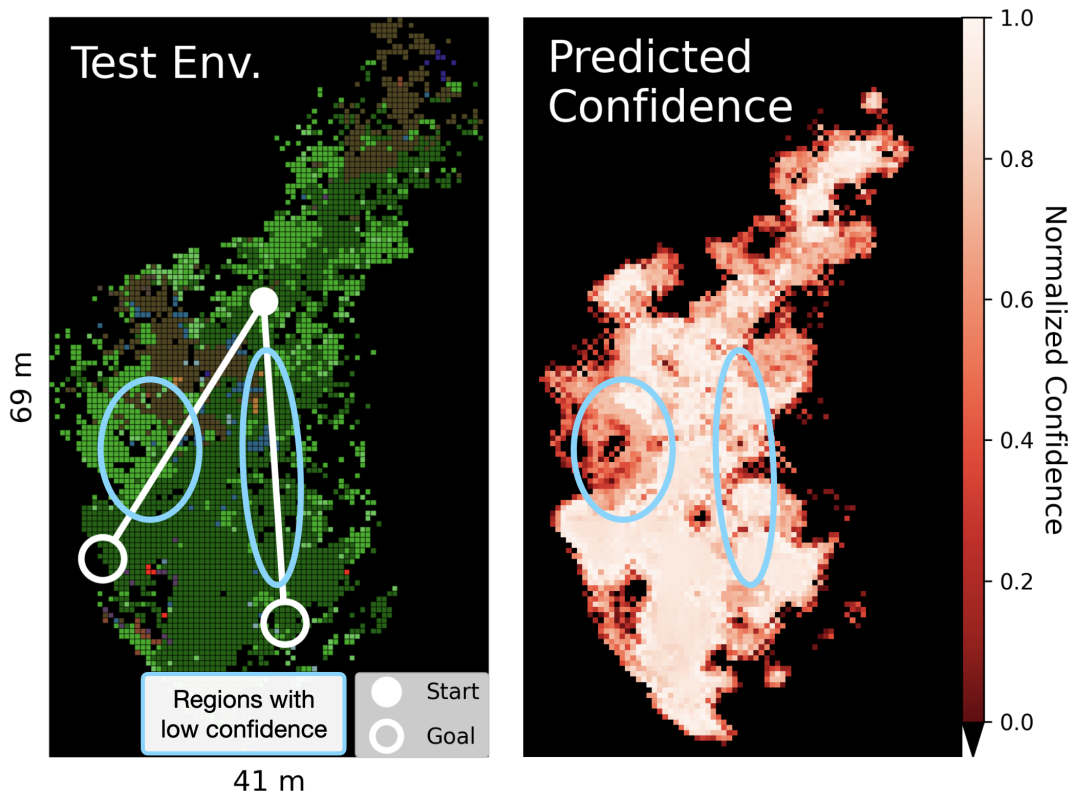
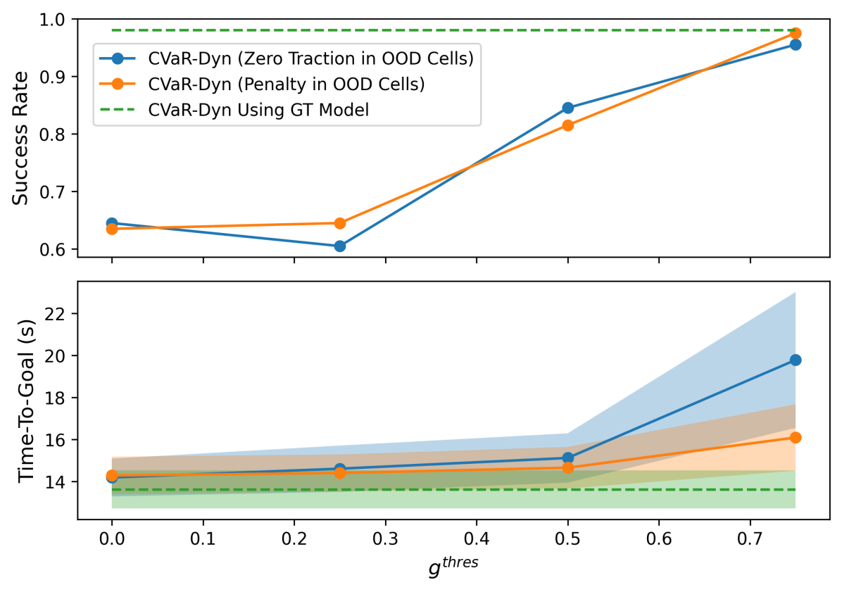
In this section, we demonstrate the benefit of the proposed density-based confidence score (8) for detecting terrains that lead to unreliable NN predictions. Because benchmarking different planning algorithms is not the main focus of this section, we use the proposed CVaR-Dyn planner that has been shown to achieve higher success rates than CVaR-Cost and set a low risk tolerance (experience has shown that similar results occur using other planners). In order to simulate training and testing environments, we leverage the data collected in two distinct forests, where the first one (visualized in Fig. 2) is used to train the traction predictor, and the second one (whose semantic top-down view is shown in Fig. 10) is used to simulate the test environment. The traction values will be drawn from the test environment’s empirical traction distribution learned by a separate NN as the proxy ground truth. Two specific start-goal pairs are selected in order to highlight the most challenging parts of the test environment with novel features. Each start-goal pair is repeated 10 times for each selected confidence threshold . We investigate two different approaches to prevent the planner from entering OOD terrains with low confidence: (1) assigning zero traction to OOD terrains, and (2) adding large penalties for states entering OOD terrains. Note that the mission is successful if each goal is reached within 30 s.
As shown in Fig. 10, the navigation success rate improves by up to as increases, because the robot avoids regions where the network’s prediction may be significantly different from the ground truth. Interestingly, using CVaR-Dyn with additional penalties for states entering OOD terrains leads to better time-to-goal while retaining similar success rate. Intuitively, the auxiliary costs make it easier for the CVaR-Dyn planner to find trajectories that move around the OOD terrains. Therefore, it is advantageous to combine the proposed cost formulations with auxiliary costs when domain knowledge is available in order to achieve both high success rate and fast navigation in practice.
VII Conclusion & Future Work
This work proposed a probabilistic traversability model that is easy to train thanks to self-supervision that captures the full empirical distribution of the traction parameters in the unicycle dynamics. For navigation tasks in simulated environments, planning with the proposed risk-aware costs led to better performance than methods that assumed no slip or used expected traction. Furthermore, the learned traction model generalized better in novel environments by avoiding terrains that had low confidence scores based on the GMM-based density estimator. Lastly, using the proposed costs with auxiliary penalties for undesirable terrains, when such prior knowledge is available, can lead to improved performance.
Based on our results, the proposed CVaR-Cost planner achieved the best time-to-goals but suffered from poor sample efficiency and conservativeness. Therefore, two interesting research directions are to design a sample-efficient planner that optimizes the CVaR of the objective, and to investigate other risk metrics that are less conservative. Additionally, the proposed framework can be streamlined by replacing the GMM with a normalizing flow model that can be jointly trained. Lastly, extensive hardware experiments are needed to validate the proposed approaches in practice.
Acknowledgment
Research was sponsored by ARL W911NF-21-2-0150 and by ONR grant N00014-18-1-2832.
References
- [1] D. D. Fan, K. Otsu, Y. Kubo, A. Dixit, J. Burdick, and A.-A. Agha-Mohammadi, “Step: Stochastic traversability evaluation and planning for risk-aware off-road navigation,” in Robotics: Science and Systems. RSS Foundation, 2021, pp. 1–21.
- [2] J. Frey, D. Hoeller, S. Khattak, and M. Hutter, “Locomotion policy guided traversability learning using volumetric representations of complex environments,” arXiv preprint arXiv:2203.15854, 2022.
- [3] A. A. Pereira, J. Binney, G. A. Hollinger, and G. S. Sukhatme, “Risk-aware path planning for autonomous underwater vehicles using predictive ocean models,” Journal of Field Robotics, vol. 30, no. 5, pp. 741–762, 2013.
- [4] M. Massari, G. Giardini, and F. Bernelli-Zazzera, “Autonomous navigation system for planetary exploration rover based on artificial potential fields,” in Proceedings of Dynamics and Control of Systems and Structures in Space (DCSSS) 6th Conference, 2004, pp. 153–162.
- [5] A. Valada, G. Oliveira, T. Brox, and W. Burgard, “Deep multispectral semantic scene understanding of forested environments using multimodal fusion,” in International Symposium on Experimental Robotics (ISER), 2016.
- [6] A. Valada, J. Vertens, A. Dhall, and W. Burgard, “Adapnet: Adaptive semantic segmentation in adverse environmental conditions,” in 2017 IEEE International Conference on Robotics and Automation (ICRA). IEEE, 2017, pp. 4644–4651.
- [7] Z. Chen, D. Pushp, and L. Liu, “Cali: Coarse-to-fine alignments based unsupervised domain adaptation of traversability prediction for deployable autonomous navigation,” arXiv preprint arXiv:2204.09617, 2022.
- [8] T. Guan, D. Kothandaraman, R. Chandra, A. J. Sathyamoorthy, K. Weerakoon, and D. Manocha, “Ga-nav: Efficient terrain segmentation for robot navigation in unstructured outdoor environments,” IEEE Robotics and Automation Letters, vol. 7, no. 3, pp. 8138–8145, 2022.
- [9] T. Guan, Z. He, R. Song, D. Manocha, and L. Zhang, “Tns: Terrain traversability mapping and navigation system for autonomous excavators,” Robotics: Science and Systems XVIII, 2021.
- [10] A. Shaban, X. Meng, J. Lee, B. Boots, and D. Fox, “Semantic terrain classification for off-road autonomous driving,” in Conference on Robot Learning. PMLR, 2022, pp. 619–629.
- [11] M. Wigness, S. Eum, J. G. Rogers, D. Han, and H. Kwon, “A rugd dataset for autonomous navigation and visual perception in unstructured outdoor environments,” in International Conference on Intelligent Robots and Systems (IROS), 2019.
- [12] P. Jiang, P. Osteen, M. Wigness, and S. Saripalli, “Rellis-3d dataset: Data, benchmarks and analysis,” in 2021 IEEE International Conference on Robotics and Automation (ICRA). IEEE, 2021, pp. 1110–1116.
- [13] G. Kahn, P. Abbeel, and S. Levine, “Badgr: An autonomous self-supervised learning-based navigation system,” IEEE Robotics and Automation Letters, vol. 6, no. 2, pp. 1312–1319, 2021.
- [14] X. Yao, J. Zhang, and J. Oh, “Rca: Ride comfort-aware visual navigation via self-supervised learning,” arXiv preprint arXiv:2207.14460, 2022.
- [15] J. Zürn, W. Burgard, and A. Valada, “Self-supervised visual terrain classification from unsupervised acoustic feature learning,” IEEE Transactions on Robotics, vol. 37, no. 2, pp. 466–481, 2020.
- [16] M. V. Gasparino, A. N. Sivakumar, Y. Liu, A. E. B. Velasquez, V. A. H. Higuti, J. Rogers, H. Tran, and G. Chowdhary, “Wayfast: Navigation with predictive traversability in the field,” IEEE Robotics and Automation Letters, vol. 7, no. 4, pp. 10 651–10 658, 2022.
- [17] X. Cai, M. Everett, J. Fink, and J. P. How, “Risk-aware off-road navigation via a learned speed distribution map,” in 2022 IEEE/RSJ International Conference on Intelligent Robots and Systems (IROS). IEEE, 2022, pp. 2931–2937.
- [18] A. J. Sathyamoorthy, K. Weerakoon, T. Guan, J. Liang, and D. Manocha, “Terrapn: Unstructured terrain navigation through online self-supervised learning,” arXiv preprint arXiv:2202.12873, 2022.
- [19] F. G. Oliveira, A. A. Neto, D. Howard, P. Borges, M. F. Campos, and D. G. Macharet, “Three-dimensional mapping with augmented navigation cost through deep learning,” Journal of Intelligent & Robotic Systems, vol. 101, no. 3, pp. 1–21, 2021.
- [20] S. Otte, C. Weiss, T. Scherer, and A. Zell, “Recurrent neural networks for fast and robust vibration-based ground classification on mobile robots,” in 2016 IEEE International Conference on Robotics and Automation (ICRA). IEEE, 2016, pp. 5603–5608.
- [21] J. Larson, M. Trivedi, and M. Bruch, “Off-road terrain traversability analysis and hazard avoidance for ugvs,” California University San Diego, Dept. of Electrical Engineering, Tech. Rep., 2011.
- [22] T. Overbye and S. Saripalli, “Fast local planning and mapping in unknown off-road terrain,” in 2020 IEEE International Conference on Robotics and Automation (ICRA). IEEE, 2020, pp. 5912–5918.
- [23] ——, “G-vom: A gpu accelerated voxel off-road mapping system,” in 2022 IEEE Intelligent Vehicles Symposium (IV). IEEE, 2022, pp. 1480–1486.
- [24] T. Guan, Z. He, D. Manocha, and L. Zhang, “Ttm: Terrain traversability mapping for autonomous excavator navigation in unstructured environments,” arXiv preprint arXiv:2109.06250, 2021.
- [25] Y. Tan, N. Virani, B. Good, S. Gray, M. Yousefhussien, Z. Yang, K. Angeliu, N. Abate, and S. Sen, “Risk-aware autonomous navigation,” in Artificial Intelligence and Machine Learning for Multi-Domain Operations Applications III, vol. 11746. International Society for Optics and Photonics, 2021, p. 117461D.
- [26] Y. Yang, X. Meng, W. Yu, T. Zhang, J. Tan, and B. Boots, “Learning semantics-aware locomotion skills from human demonstration,” arXiv preprint arXiv:2206.13631, 2022.
- [27] D. D. Fan, A.-A. Agha-Mohammadi, and E. A. Theodorou, “Learning risk-aware costmaps for traversability in challenging environments,” IEEE Robotics and Automation Letters, vol. 7, no. 1, pp. 279–286, 2021.
- [28] Z. Wang, O. So, K. Lee, and E. A. Theodorou, “Adaptive risk sensitive model predictive control with stochastic search,” in Learning for Dynamics and Control. PMLR, 2021, pp. 510–522.
- [29] J. Gawlikowski, C. R. N. Tassi, M. Ali, J. Lee, M. Humt, J. Feng, A. Kruspe, R. Triebel, P. Jung, R. Roscher, et al., “A survey of uncertainty in deep neural networks,” arXiv preprint arXiv:2107.03342, 2021.
- [30] Y. Gal and Z. Ghahramani, “Dropout as a bayesian approximation: Representing model uncertainty in deep learning,” in international conference on machine learning. PMLR, 2016, pp. 1050–1059.
- [31] I. Osband, C. Blundell, A. Pritzel, and B. Van Roy, “Deep exploration via bootstrapped dqn,” Advances in neural information processing systems, vol. 29, 2016.
- [32] B. Charpentier, O. Borchert, D. Zügner, S. Geisler, and S. Günnemann, “Natural Posterior Network: Deep Bayesian Predictive Uncertainty for Exponential Family Distributions,” in International Conference on Learning Representations, 2022.
- [33] G. Williams, N. Wagener, B. Goldfain, P. Drews, J. M. Rehg, B. Boots, and E. A. Theodorou, “Information theoretic mpc for model-based reinforcement learning,” in 2017 IEEE International Conference on Robotics and Automation (ICRA). IEEE, 2017, pp. 1714–1721.
- [34] A. Asgharivaskasi and N. Atanasov, “Active bayesian multi-class mapping from range and semantic segmentation observations,” in 2021 IEEE International Conference on Robotics and Automation (ICRA). IEEE, 2021, pp. 1–7.
- [35] A. Kirillov, Y. Wu, K. He, and R. Girshick, “Pointrend: Image segmentation as rendering,” in Proceedings of the IEEE/CVF conference on computer vision and pattern recognition, 2020, pp. 9799–9808.
- [36] K. Chen, B. T. Lopez, A.-a. Agha-mohammadi, and A. Mehta, “Direct lidar odometry: Fast localization with dense point clouds,” IEEE Robotics and Automation Letters, vol. 7, no. 2, pp. 2000–2007, 2022.
- [37] A. Majumdar and M. Pavone, “How should a robot assess risk? towards an axiomatic theory of risk in robotics,” in Robotics Research. Springer, 2020, pp. 75–84.