Probabilistic Transformer: A Probabilistic Dependency Model for Contextual Word Representation

Given a sentence (a sequence of words), denote $n$ as the sequence length. For the $i$-th word, we define $Z_{i}$ as a discrete latent label that represents the syntactic (and possibly semantic) property of the word in the sentence (i.e., it is a contextual representation) with a label set of size $d$. Such a discrete representation deviates from the common practice of representing a word with a continuous vector, but it is sufficient at least for syntactic processing Kitaev et al. (2022) and it greatly simplifies our probabilistic model. For the $i$-th word, we also define $H_{i}\in\{1,2,\cdots,n\}$ representing the syntactic dependency head of the word. So the set of variables $\{H_{i}\}_{i=1}^{n}$ specifies a dependency structure. We may also allow $H_{i}$ to point to a dummy root node, which will be discussed in Section 2.3.5. We follow the head-selection paradigm of dependency parsing and do not enforce the tree constraint, which again simplifies our model design.

Next, we define two types of potential functions. For the $i$-th word $w_{i}$, we define a unary potential function (corresponding to the unary factors in Figure 1) evaluating the compatibility of the word and its label $Z_{i}$:

where $\mathbf{S}\in\mathbb{R}^{|\mathcal{V}|\times d}$ is a score matrix, $|\mathcal{V}|$ is the size of the vocabulary. For simplicity, we do not exploit any morphological or contextual features for computing the scores. For every pair of words $w_{i}$ and $w_{j}$ ($i\neq j$), we define a ternary potential function (corresponding to the ternary factors in Figure 1) over $Z_{i}$, $Z_{j}$ and $H_{i}$, which evaluates the compatibility between the labels of the two words if $w_{j}$ is the dependency head of $w_{i}$:

where $\mathbf{T}\in\mathbb{R}^{d\times d}$ is a score matrix.

Inspired by the multi-head structure in transformers, we allow multiple dependency structures for the same sentence, which may represent different flavors of dependencies. Each dependency structure resides in a different channel with its own dependency head variables and ternary potential functions. For the $c$-th channel, we denote the set of dependency head variables by $\{H_{i}^{(c)}\}_{i=1}^{n}$ and the score matrix of the ternary potential function by $\mathbf{T}^{(c)}$. Let $h$ denote the total number of channels. We may stack all the score matrices $\mathbf{T}^{(c)}$ for $c=1,\cdots,h$ to form a score tensor $\mathbf{T}\in\mathbb{R}^{d\times d\times h}$. Note that all the channels share the same set of latent label variables $\{Z_{i}\}_{i=1}^{n}$.

Following Wang and Tu (2020), we use Mean Field Variational Inference (MFVI) to perform approximate inference. Different from the previous work, however, we need to run inference over latent labels in addition to dependency heads.

MFVI iteratively passes messages between random variables and computes an approximate posterior marginal distribution for each random variable (denoted by $Q(\cdot)$). Let $\mathcal{F}_{ic}^{(t)}$ denote the message received by variable $H_{i}^{(c)}$ at time step $t$ from ternary factors, and $\mathcal{G}_{i}^{(t)}$ denote the message received by variable $Z_{i}$ at time step $t$ from ternary factors. We have

where

are the approximate marginal distributions at time step $t$, with $Q_{i}^{(t)}(\cdot)$ over $Z_{i}$ and $Q_{ic}^{(t)}(\cdot)$ over $H_{i}^{(c)}$. We initialize these distributions by

After a fixed number of $T>0$ iterations, we obtain the final posterior marginal distribution $Q_{i}^{(T)}(Z_{i})$ for $i=1,\cdots,n$. Resulted from interactions with all the words of the sentence, the distribution $Q_{i}^{(T)}(Z_{i})$ incorporates information of not only the $i$-th word, but also its context. Therefore, we can treat the probability vector of this distribution as a contextual vector representation for the $i$-th word. In practice, we find that using unnormalized scores in log space as contextual word representations produces better results, i.e., we skip exponentiation and normalization when computing $Q_{i}^{(T)}(Z_{i})$ using Equation 5 during the final iteration.

Since all the computation during MFVI is fully differentiable, we can regard the corresponding computation graph as a recurrent or graph neural network parameterized with score matrix $\mathbf{S}$ and tensor $\mathbf{T}$. We can use the contextual word representations for downstream tasks by connecting the network to any downstream task-specific network, and we can update the model parameters using any task-specific learning objective through gradient descent. This is exactly the same as how transformers are used.

We introduce a few extensions and variants to the basic model that are empirically beneficial. Additional variants are discussed in Appendix B.

Consider a probabilistic transformer using a distance-insensitive ternary potential function without a dummy root node. We tensorize the update formulas in the inference process of probabilistic transformers. Suppose $Q_{z}^{(t)}\in\mathbb{R}^{n\times d}$ is a tensor that represents the posterior distributions of all the $Z$ variables, and $Q_{h,c}^{(t)}\in\mathbb{R}^{n\times n}$ is a tensor that represents the posterior distributions of all the $H$ variables in channel $c$ (with a zero diagonal to rule out self-heading). We can rewrite Equation 3 and 4 as

where

and $\sigma$ is the softmax function. We still set $\lambda_{Z}$ to its default value $1$ but regard $\lambda_{H}$ as a hyperparameter. With asynchronous update, Equation 18 becomes:

We assume that $\mathbf{T}^{(c)}$ is symmetric for $c=1,\cdots,h$. This is the only assumption that we make in this section beyond the original definition from the previous section. Symmetric score matrices indicate that the ternary factors are insensitive to the head-child order, which is related to undirected dependency parsing Sleator and Temperley (1993). If $\mathbf{T}^{(c)}$ is symmetric, then $Q_{h,c}^{(t)}$ is also symmetric based on Formula 15 and 19. Thus, we can simplify Equation 16 to

Suppose we decompose the ternary score tensor into two tensors $\mathbf{U},\mathbf{V}\in\mathbb{R}^{d\times h\times r}$ according to Equation 14, which can be rewritten as:

where $\mathbf{U}^{(c)},\mathbf{V}^{(c)}\in\mathbb{R}^{d\times r}$ are the $c$-th channel of tensor $\mathbf{U}$ and $\mathbf{V}$ respectively. Substitute 21 into 15 and 20, we have

We define

For time step $t-1$, we could rewrite Formula 22 and 23 as

Apply Equation 27, 19, 26 to 17, we have

where

We call the computation of $\operatorname{channel}_{c}$ a single-channel update for channel $c$.

Now we have a tensorized formulation of the computation in probabilistic transformers and we are ready for its comparison with transformers at three different levels.

Scaled dot-product attention in transformers is formulated as:

As we can see, our single-channel update in Equation 29 is almost identical to scaled dot-product attention in transformers. The only difference is that the diagonal of the tensor $Q_{c}K_{c}^{T}$ is zero in our model because the head of a word cannot be itself.

Multi-head attention in transformers is formulated as:

where

It is equivalent to

where $W^{O}\equiv\operatorname{Concat}(W_{1}^{O},\ldots,W_{h}^{O})$ and $W_{i}^{Q},W_{i}^{K},W_{i}^{V},W_{i}^{O}\in\mathbb{R}^{d\times r}$. Our multi-channel update formula (the second term within the softmax function in Equation 28) is similar to the multi-head attention in transformers, as shown in Figure 2. The main difference is that probabilistic transformers use the same parameters for $W^{K}$ and $W^{V}$ (both are $\mathbf{V}$, shown in green color in Figure 2(b)) and for $W^{Q}$ and $W^{O}$ (both are $\mathbf{U}$, shown in orange color in Figure 2(b)).

Recall that $\mathbf{U}$ and $\mathbf{V}$ are obtained from matrix decomposition (Equation 14). Therefore, the correspondence between $\mathbf{U}$, $\mathbf{V}$ and $W^{Q},W^{K},W^{O},W^{V}$ in transformers suggests that the latter can also be seen as derived from tensor decomposition. Previous work on transformers has the same findings Elhage et al. (2021).

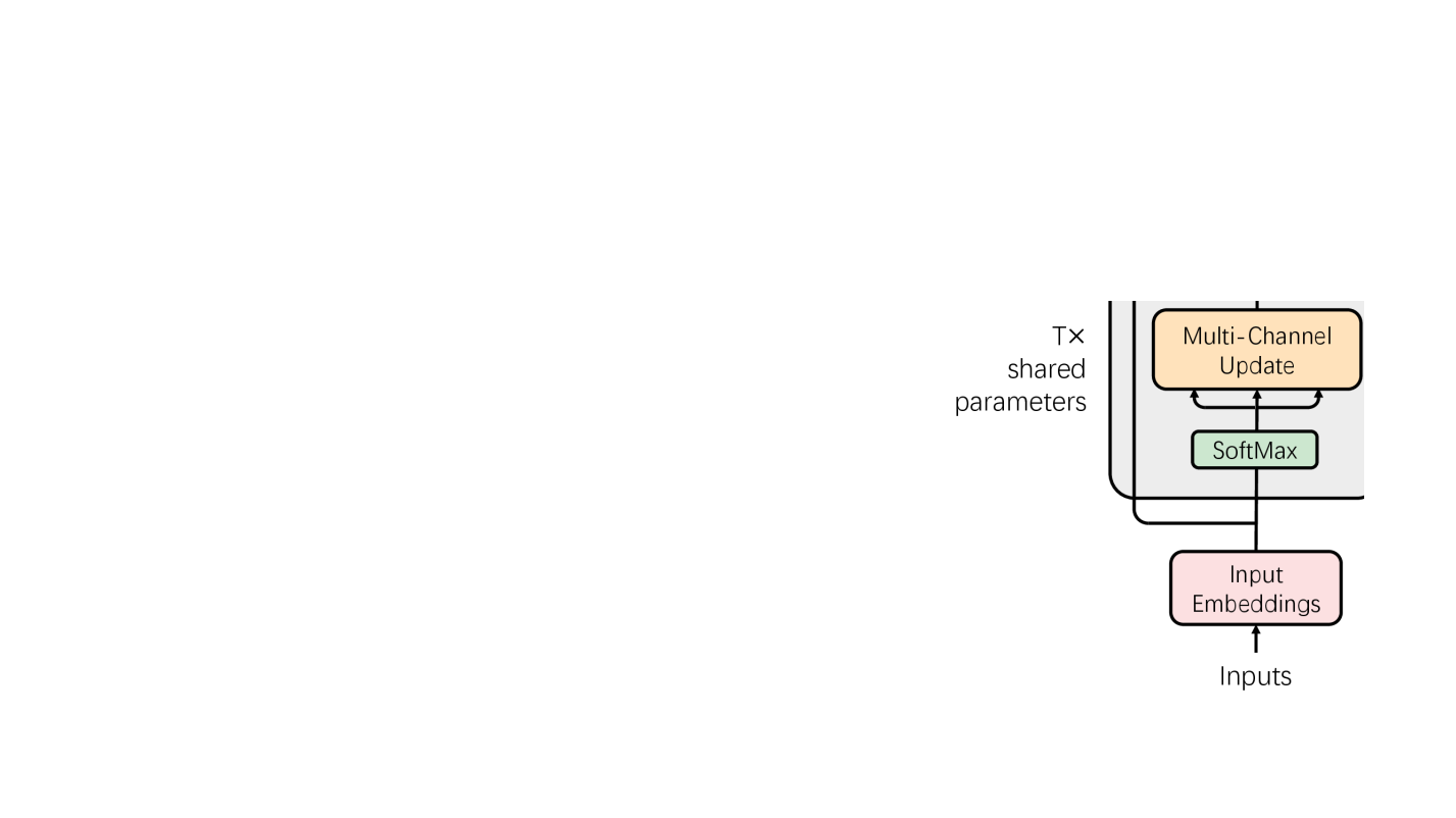
Figure 3 compares the full computation graphs of the two models, which have a similar overall structure that repeats a module recurrently until outputting contextual word representations. Within the module, we have also established the correspondence between multi-channel update and multi-head attention. On the other hand, there are a few interesting differences.

First, our model does not have a feed-forward structure as in a transformer. However, we do propose a variant of our model that contains global variables representing topics (Appendix B.3), which may have similar functionality to the feed-forward structure.

Second, our model does not have residual connections or layer norms. Instead, it adds the initial distributions (unary scores) to the updated message at each iteration. This may replace the functionality of residual connections and may even make more sense when the downstream task strongly depends on the original word information.

Third, we have an additional softmax in each iteration. Note that we do softmax before the first iteration (Equation 7) and also at the end of each iteration (Equation 28), but bypass it in the last iteration when producing the output word representations, so our model could be equivalently formulated as doing softmax before each iteration, which we show in Figure 3(c). Doing softmax in this way is similar to the layer norm in pre-LN transformers Xiong et al. (2020) (Figure 3(b)).

Finally, our model shares parameters in all iterations. This is similar to some variants of transformers that share parameters between layers, such as Universal Transformer Dehghani et al. (2019) and ALBERT Lan et al. (2019).

One consequence of these differences is that probabilistic transformers have much fewer parameters than transformers with the same number of layers, heads and embedding dimensions, because of shared parameters between iterations, absence of a feed-forward structure, and tied parameter matrices in multi-channel updates.

Here we briefly introduce our tasks and datasets. A detailed description is presented in Appendix D.

Masked Language Modeling (MLM). We perform MLM tasks on two corpora: the Penn TreeBank (PTB) Marcus et al. (1993) and Brown Laboratory for Linguistic Information Processing (BLLIP) Charniak et al. (2000). Following Shen et al. (2022), we randomly replace words with a mask token <mask> at a rate of 30%. The performance of MLM is evaluated by measuring perplexity (lower is better) on masked words.

We project the final word representation of each mask token to the vocabulary. For transformers, we tie the projection parameters to the initial word embeddings. We find that this trick improves the performance of transformers.

Sequence Labeling. For sequence labeling tasks, we perform part-of-speech (POS) tagging on two datasets: the Penn TreeBank (PTB) Marcus et al. (1993) and the Universal Dependencies (UD) De Marneffe et al. (2021). We also perform named entity recognition (NER) on CoNLL-2003 Tjong Kim Sang and De Meulder (2003).

We directly project the final word representation of each word to the target tag set. For POS tagging, we evaluate the results by the accuracy of word-level predictions. For NER, we evaluate the results by measuring the F1 score of named entities.

Text Classification. We use the Stanford Sentiment Treebank (SST) Socher et al. (2013) as the dataset. It has two variants: binary classification (SST-2) and fine-grained classification (SST-5).

For transformers, we add a <CLS> token at the front of the sentence and then project its representation to the tag set. For our model, we use the variant with a root node introduced in Section 2.3.5 and project the representation of the root node to the tag set.

Syntactic Test. To evaluate the compositional generalization abilities of our model, we perform a syntactic test on the COGS dataset Kim and Linzen (2020). We follow the settings in Ontanón et al. (2021), who cast the task as a sequence labeling task.

As in sequence labeling, we project word representations to tag sets. If all words in a sentence are correctly predicted, the sentence prediction will be counted as correct. We evaluate the results by the sentence-level accuracy of the predictions.

We tune transformers and our model separately for each task except the syntactic test. For the syntactic test, we find that both transformers and our model easily reach 100% accuracy on the validation set. This observation is consistent with Ontanón et al. (2021). Therefore, instead of tuning, we use the best-performed setting of transformers in Ontanón et al. (2021) for our experiments. The hyperparameters of our model are determined by their counterparts of transformers based on the correspondence discussed in Section 3.

For our model, we integrate all the variants mentioned in Section 2.3 except the root node variant, which we only use for text classification tasks. We tune the tensor decomposition strategy on different tasks. For MLM tasks, we add a small L2 regularization term to the ternary scores in our model, which we experimentally find beneficial. We optimize both models using the Adam optimizer Kingma and Ba (2015) with $\beta_{1}=0.9$, $\beta_{2}=0.999$.

We report the average and standard deviation results of 5 random runs in Table 1. It shows that our model has a competitive performance compared with transformers. In most tasks, probabilistic transformers perform competitively to transformers. It is worth noting that in these experiments, probabilistic transformers have much fewer parameters than transformers. For most tasks, the number of parameters of our best model is about one-fifth to one-half of that of the best transformer.

We also conduct case studies of the dependency structures inferred by our model after training on downstream tasks. Similar to the case of self-attentions in transformers, the inferred dependency structures are only partially consistent with human intuition. See Appendix F for details.

References

- Ahmad et al. (2021) Wasi Uddin Ahmad, Nanyun Peng, and Kai-Wei Chang. 2021. Gate: graph attention transformer encoder for cross-lingual relation and event extraction. In Proceedings of the AAAI Conference on Artificial Intelligence, volume 35, pages 12462–12470.
- Akbik et al. (2019) Alan Akbik, Tanja Bergmann, Duncan Blythe, Kashif Rasul, Stefan Schweter, and Roland Vollgraf. 2019. FLAIR: An easy-to-use framework for state-of-the-art NLP. In Proceedings of the 2019 Conference of the North American Chapter of the Association for Computational Linguistics (Demonstrations), pages 54–59, Minneapolis, Minnesota. Association for Computational Linguistics.
- Charniak et al. (2000) Eugene Charniak, Don Blaheta, Niyu Ge, Keith Hall, and Mark Johnson. 2000. Bllip 1987–89 wsj corpus release 1, ldc no. LDC2000T43. Linguistic Data Consortium.
- Clark et al. (2019) Kevin Clark, Urvashi Khandelwal, Omer Levy, and Christopher D. Manning. 2019. What does BERT look at? an analysis of BERT’s attention. In Proceedings of the 2019 ACL Workshop BlackboxNLP: Analyzing and Interpreting Neural Networks for NLP, pages 276–286, Florence, Italy. Association for Computational Linguistics.
- Conneau and Kiela (2018) Alexis Conneau and Douwe Kiela. 2018. Senteval: An evaluation toolkit for universal sentence representations. arXiv preprint arXiv:1803.05449.
- De Marneffe et al. (2021) Marie-Catherine De Marneffe, Christopher D Manning, Joakim Nivre, and Daniel Zeman. 2021. Universal dependencies. Computational linguistics, 47(2):255–308.
- Dehghani et al. (2019) Mostafa Dehghani, Stephan Gouws, Oriol Vinyals, Jakob Uszkoreit, and Lukasz Kaiser. 2019. Universal transformers. In International Conference on Learning Representations.
- Devlin et al. (2019) Jacob Devlin, Ming-Wei Chang, Kenton Lee, and Kristina Toutanova. 2019. Bert: Pre-training of deep bidirectional transformers for language understanding. In Proceedings of the 2019 Conference of the North American Chapter of the Association for Computational Linguistics: Human Language Technologies, Volume 1 (Long and Short Papers), pages 4171–4186.
- Dinarelli and Grobol (2019) Marco Dinarelli and Loïc Grobol. 2019. Seq2biseq: Bidirectional output-wise recurrent neural networks for sequence modelling. arXiv preprint arXiv:1904.04733.
- Dong et al. (2021) Yihe Dong, Jean-Baptiste Cordonnier, and Andreas Loukas. 2021. Attention is not all you need: pure attention loses rank doubly exponentially with depth. In Proceedings of the 38th International Conference on Machine Learning, volume 139 of Proceedings of Machine Learning Research, pages 2793–2803. PMLR.
- Elhage et al. (2021) N Elhage, N Nanda, C Olsson, T Henighan, N Joseph, B Mann, A Askell, Y Bai, A Chen, T Conerly, et al. 2021. A mathematical framework for transformer circuits. Transformer Circuits Thread.
- Geva et al. (2022) Mor Geva, Avi Caciularu, Kevin Ro Wang, and Yoav Goldberg. 2022. Transformer feed-forward layers build predictions by promoting concepts in the vocabulary space. arXiv preprint arXiv:2203.14680.
- Geva et al. (2021) Mor Geva, Roei Schuster, Jonathan Berant, and Omer Levy. 2021. Transformer feed-forward layers are key-value memories. In Proceedings of the 2021 Conference on Empirical Methods in Natural Language Processing, pages 5484–5495, Online and Punta Cana, Dominican Republic. Association for Computational Linguistics.
- He et al. (2021) Ruining He, Anirudh Ravula, Bhargav Kanagal, and Joshua Ainslie. 2021. RealFormer: Transformer likes residual attention. In Findings of the Association for Computational Linguistics: ACL-IJCNLP 2021, pages 929–943, Online. Association for Computational Linguistics.
- Hewitt and Manning (2019) John Hewitt and Christopher D. Manning. 2019. A structural probe for finding syntax in word representations. In Proceedings of the 2019 Conference of the North American Chapter of the Association for Computational Linguistics: Human Language Technologies, Volume 1 (Long and Short Papers), pages 4129–4138, Minneapolis, Minnesota. Association for Computational Linguistics.
- Htut et al. (2019) Phu Mon Htut, Jason Phang, Shikha Bordia, and Samuel R Bowman. 2019. Do attention heads in bert track syntactic dependencies? arXiv preprint arXiv:1911.12246.
- Hu et al. (2020) Jennifer Hu, Jon Gauthier, Peng Qian, Ethan Wilcox, and Roger Levy. 2020. A systematic assessment of syntactic generalization in neural language models. In Proceedings of the 58th Annual Meeting of the Association for Computational Linguistics, pages 1725–1744, Online. Association for Computational Linguistics.
- Kim and Linzen (2020) Najoung Kim and Tal Linzen. 2020. COGS: A compositional generalization challenge based on semantic interpretation. In Proceedings of the 2020 Conference on Empirical Methods in Natural Language Processing (EMNLP), pages 9087–9105, Online. Association for Computational Linguistics.
- Kingma and Ba (2015) Diederik P. Kingma and Jimmy Ba. 2015. Adam: A method for stochastic optimization. In 3rd International Conference on Learning Representations, ICLR 2015, San Diego, CA, USA, May 7-9, 2015, Conference Track Proceedings.
- Kitaev et al. (2022) Nikita Kitaev, Thomas Lu, and Dan Klein. 2022. Learned incremental representations for parsing. In Proceedings of the 60th Annual Meeting of the Association for Computational Linguistics (Volume 1: Long Papers), pages 3086–3095, Dublin, Ireland. Association for Computational Linguistics.
- Lan et al. (2019) Zhenzhong Lan, Mingda Chen, Sebastian Goodman, Kevin Gimpel, Piyush Sharma, and Radu Soricut. 2019. Albert: A lite bert for self-supervised learning of language representations. In International Conference on Learning Representations, pages 1–16.
- Lê-Huu and Alahari (2021) Đ Khuê Lê-Huu and Karteek Alahari. 2021. Regularized frank-wolfe for dense crfs: Generalizing mean field and beyond. Advances in Neural Information Processing Systems, 34:1453–1467.
- Liu et al. (2020) Yinhan Liu, Myle Ott, Naman Goyal, Jingfei Du, Mandar Joshi, Danqi Chen, Omer Levy, Mike Lewis, Luke Zettlemoyer, and Veselin Stoyanov. 2020. Roberta: A robustly optimized bert pretraining approach. In International Conference on Learning Representations, pages 1–15.
- Marcus et al. (1993) Mitchell P. Marcus, Mary Ann Marcinkiewicz, and Beatrice Santorini. 1993. Building a large annotated corpus of english: The penn treebank. Comput. Linguist., 19(2):313–330.
- Mikolov et al. (2012) Tomáš Mikolov et al. 2012. Statistical language models based on neural networks. Presentation at Google, Mountain View, 2nd April, 80:26.
- Ontanón et al. (2021) Santiago Ontanón, Joshua Ainslie, Vaclav Cvicek, and Zachary Fisher. 2021. Making transformers solve compositional tasks. arXiv preprint arXiv:2108.04378.
- Ravishankar et al. (2021) Vinit Ravishankar, Artur Kulmizev, Mostafa Abdou, Anders Søgaard, and Joakim Nivre. 2021. Attention can reflect syntactic structure (if you let it). In Proceedings of the 16th Conference of the European Chapter of the Association for Computational Linguistics: Main Volume, pages 3031–3045, Online. Association for Computational Linguistics.
- Shaw et al. (2018) Peter Shaw, Jakob Uszkoreit, and Ashish Vaswani. 2018. Self-attention with relative position representations. In Proceedings of the 2018 Conference of the North American Chapter of the Association for Computational Linguistics: Human Language Technologies, Volume 2 (Short Papers), pages 464–468, New Orleans, Louisiana. Association for Computational Linguistics.
- Shen et al. (2022) Yikang Shen, Shawn Tan, Alessandro Sordoni, Peng Li, Jie Zhou, and Aaron Courville. 2022. Unsupervised dependency graph network. In Proceedings of the 60th Annual Meeting of the Association for Computational Linguistics (Volume 1: Long Papers), pages 4767–4784, Dublin, Ireland. Association for Computational Linguistics.
- Shen et al. (2021) Yikang Shen, Yi Tay, Che Zheng, Dara Bahri, Donald Metzler, and Aaron Courville. 2021. StructFormer: Joint unsupervised induction of dependency and constituency structure from masked language modeling. In Proceedings of the 59th Annual Meeting of the Association for Computational Linguistics and the 11th International Joint Conference on Natural Language Processing (Volume 1: Long Papers), pages 7196–7209, Online. Association for Computational Linguistics.
- Shimony (1994) Solomon Eyal Shimony. 1994. Finding maps for belief networks is np-hard. Artificial intelligence, 68(2):399–410.
- Sleator and Temperley (1993) Daniel D. Sleator and Davy Temperley. 1993. Parsing English with a link grammar. In Proceedings of the Third International Workshop on Parsing Technologies, pages 277–292, Tilburg, Netherlands and Durbuy, Belgium. Association for Computational Linguistics.
- Socher et al. (2013) Richard Socher, Alex Perelygin, Jean Wu, Jason Chuang, Christopher D. Manning, Andrew Ng, and Christopher Potts. 2013. Recursive deep models for semantic compositionality over a sentiment treebank. In Proceedings of the 2013 Conference on Empirical Methods in Natural Language Processing, pages 1631–1642, Seattle, Washington, USA. Association for Computational Linguistics.
- Strubell et al. (2018) Emma Strubell, Patrick Verga, Daniel Andor, David Weiss, and Andrew McCallum. 2018. Linguistically-informed self-attention for semantic role labeling. In Proceedings of the 2018 Conference on Empirical Methods in Natural Language Processing, pages 5027–5038, Brussels, Belgium. Association for Computational Linguistics.
- Sukhbaatar et al. (2019) Sainbayar Sukhbaatar, Edouard Grave, Guillaume Lample, Herve Jegou, and Armand Joulin. 2019. Augmenting self-attention with persistent memory. arXiv preprint arXiv:1907.01470.
- Tenney et al. (2019) Ian Tenney, Patrick Xia, Berlin Chen, Alex Wang, Adam Poliak, R Thomas McCoy, Najoung Kim, Benjamin Van Durme, Sam Bowman, Dipanjan Das, and Ellie Pavlick. 2019. What do you learn from context? probing for sentence structure in contextualized word representations. In International Conference on Learning Representations.
- Tjong Kim Sang and De Meulder (2003) Erik F. Tjong Kim Sang and Fien De Meulder. 2003. Introduction to the CoNLL-2003 shared task: Language-independent named entity recognition. In Proceedings of the Seventh Conference on Natural Language Learning at HLT-NAACL 2003, pages 142–147.
- Vaswani et al. (2017) Ashish Vaswani, Noam Shazeer, Niki Parmar, Jakob Uszkoreit, Llion Jones, Aidan N Gomez, Łukasz Kaiser, and Illia Polosukhin. 2017. Attention is all you need. Advances in neural information processing systems, 30.
- Wang and Tu (2020) Xinyu Wang and Kewei Tu. 2020. Second-order neural dependency parsing with message passing and end-to-end training. In Proceedings of the 1st Conference of the Asia-Pacific Chapter of the Association for Computational Linguistics and the 10th International Joint Conference on Natural Language Processing, pages 93–99, Suzhou, China. Association for Computational Linguistics.
- Wang et al. (2019) Yaushian Wang, Hung-Yi Lee, and Yun-Nung Chen. 2019. Tree transformer: Integrating tree structures into self-attention. In Proceedings of the 2019 Conference on Empirical Methods in Natural Language Processing and the 9th International Joint Conference on Natural Language Processing (EMNLP-IJCNLP), pages 1061–1070, Hong Kong, China. Association for Computational Linguistics.
- Xiong et al. (2020) Ruibin Xiong, Yunchang Yang, Di He, Kai Zheng, Shuxin Zheng, Chen Xing, Huishuai Zhang, Yanyan Lan, Liwei Wang, and Tieyan Liu. 2020. On layer normalization in the transformer architecture. In International Conference on Machine Learning, pages 10524–10533. PMLR.
Appendix A Extended Entropic Frank-Wolfe
In Section 2.3.3, we add message weights to the update function of the posterior marginal distributions. It follows an extension of the Entropic Frank-Wolfe algorithm Lê-Huu and Alahari (2021), which is a generalization of MFVI. Below we briefly introduce the algorithm and our extension following most of the notations in their paper.
A.1 Entropic Frank-Wolfe
Suppose we want to minimize a continuous differentiable energy function . Vanilla Frank-Wolfe solves the problem by starting from a feasible at time step 0, and iterating the following steps:
where follows some stepsize scheme, is the value range of , and here we let be the concatenation of the distributions over the label set of all variables in CRF.
Regularized Frank-Wolfe Lê-Huu and Alahari (2021) adds a regularization term to the objective. It solves the new objective by iterating
It has been proved that regularized Frank-Wolfe achieves a sublinear rate of convergence for suitable stepsize schemes.
Entropic Frank-Wolfe is a special case of regularized Frank-Wolfe, which sets the regularization term as an entropy function , where , is the label set of the variables, is the set of indices of the variables. Entropy Frank-Wolfe has a closed-form solution for the update process