Probabilistic Metric Learning with Adaptive Margin for Top-K Recommendation
Abstract.
Personalized recommender systems are playing an increasingly important role as more content and services become available and users struggle to identify what might interest them. Although matrix factorization and deep learning based methods have proved effective in user preference modeling, they violate the triangle inequality and fail to capture fine-grained preference information. To tackle this, we develop a distance-based recommendation model with several novel aspects: (i) each user and item are parameterized by Gaussian distributions to capture the learning uncertainties; (ii) an adaptive margin generation scheme is proposed to generate the margins regarding different training triplets; (iii) explicit user-user/item-item similarity modeling is incorporated in the objective function. The Wasserstein distance is employed to determine preferences because it obeys the triangle inequality and can measure the distance between probabilistic distributions. Via a comparison using five real-world datasets with state-of-the-art methods, the proposed model outperforms the best existing models by 4-22% in terms of recall@K on Top-K recommendation.
1. Introduction
Internet users can easily access an increasingly vast number of online products and services, and it is becoming very difficult for users to identify the items that will appeal to them out of a plethora of candidates. To reduce information overload and to satisfy the diverse needs of users, personalized recommender systems have emerged and they are beginning to play an important role in modern society. These systems can provide personalized experiences, serve huge service demands, and benefit both the user-side and supply-side. They can: (i) help users easily discover products that are likely to interest them; and (ii) create opportunities for product and service providers to better serve customers and to increase revenue.
In all kinds of recommender systems, modeling the user-item interaction lies at the core. There are two common ways used in recent recommendation models to infer the user preference: matrix factorization (MF) and multi-layer perceptrons (MLPs). MF-based methods (e.g., (Hu et al., 2008; Rendle et al., 2009)) apply the inner product between latent factors of users and items to predict the user preferences for different items. The latent factors strive to depict the user-item relationships in the latent space. In contrast, MLP-based methods (e.g., (He et al., 2017b; Covington et al., 2016)) adopt (deep) neural networks to learn non-linear user-item relationships, which can generate better latent feature combinations between the embeddings of users and items (He et al., 2017b).
However, both MF-based and MLP-based methods violate the triangle inequality (Shrivastava and Li, 2014), and as a result may fail to capture the fine-grained preference information (Hsieh et al., 2017). As a concrete example in (Park et al., 2018), if a user accessed two items, MF or MLP-based methods will put both items close to the user, but will not necessarily put these two items close to each other, even if they share similar properties.
To address the limitations of MF and MLP-based methods, metric (distance) learning approaches have been utilized in the recommendation model (Hsieh et al., 2017; Park et al., 2018; Tay et al., 2018; Li et al., 2020), as the distance naturally satisfies the triangle inequality. These techniques project users and items into a low-dimensional metric space, where the user preference is measured by the distance to items. Specifically, CML (Hsieh et al., 2017) and LRML (Tay et al., 2018) are two representative models. CML minimizes the Euclidean distance between users and their accessed items, which facilitates user-user/item-item similarity learning. LRML incorporates a memory network to introduce additional capacity to learn relations between users and items in the metric space.

Although existing distance-based methods have achieved satisfactory results, we argue that there are still several avenues for enhancing performance. First, previous distance-based methods (Hsieh et al., 2017; Park et al., 2018; Tay et al., 2018; Li et al., 2020) learn the user and item embeddings in a deterministic manner without handling the uncertainty. Relying solely on the learned deterministic embeddings may lead to an inaccurate understanding of user preferences. A motivating example is shown in Figure 1. After having accessed two songs and with different genres, the user may be placed between of and . If we only consider deterministic embeddings, should be a good candidate. But if we consider the embeddings from a probabilistic perspective, can be a better recommendation and it has the same genre as . Second, most of the existing methods (Hsieh et al., 2017; Tay et al., 2018; Park et al., 2018) adopt the margin ranking loss (hinge loss) with a fixed margin as the hyper-parameter. We argue that the margin value should be adaptive and relevant to corresponding training samples. Furthermore, different training phases may need different magnitudes of margin values. Setting a fixed value may not be an optimal solution. Third, previous distance-based methods (Hsieh et al., 2017; Tay et al., 2018; Park et al., 2018; Li et al., 2020) do not explicitly model user-user and item-item relationships. Closely-related users are very likely to share the same interests, and if two items have similar attributes it is likely that a user will favour both. When inferring a user’s preferences, we should explicitly take into account the user-user and item-item similarities.
To address the shortcomings, we propose a Probabilistic Metric Learning model with an Adaptive Margin (PMLAM) for Top-K recommendation. PMLAM consists of three major components: 1) a user-item interaction module, 2) an adaptive margin generation module, and 3) a user-user/item-item relation modeling module. To capture the uncertainties in the learned user and item embeddings, each user or item is parameterized with one Gaussian distribution, where the distribution related parameters are learned by our model. In the user-item interaction module, we adopt the Wasserstein distance to measure the distances between users and items, thus not only taking into account the means but also the uncertainties. In the adaptive margin generation module, we model the learning of adaptive margins as a bilevel (inner and outer) optimization problem (Sinha et al., 2018), where we build a proxy function to explicitly link the learning of margin related parameters with the outer objective function. In the user-user and item-item relation modeling module, we incorporate two margin ranking losses with adaptive margins for user-pairs and item-pairs, respectively, to explicitly encourage similar users or items to be mapped closer to one another in the latent space. We extensively evaluate our model by comparing with many state-of-the-art methods, using two performance metrics on five real-world datasets. The experimental results not only demonstrate the improvements of our model over other baselines but also show the effectiveness of the proposed modules.
To summarize, the major contributions of this paper are:
-
•
To capture the uncertainties in the learned user/item embeddings, we represent each user and item as a Gaussian distribution. The Wasserstein distance is leveraged to measure the user preference for items while simultaneously considering the uncertainty.
-
•
To generate an adaptive margin, we cast margin generation as a bilevel optimization problem, where a proxy function is built to explicitly update the margin generation related parameters.
-
•
To explicitly model the user-user and item-item relationships, we apply two margin ranking losses with adaptive margins to force similar users and items to map closer to one another in the latent space.
-
•
Experiments on five real-world datasets show that the proposed PMLAM model significantly outperforms the state-of-the-art methods for the Top-K recommendation task.
2. Related Work
In this section we summarize and discuss work that is related to our proposed top-K recommendation model.
In many real-world recommendation scenarios, user implicit data (Wang et al., 2015; Ma et al., 2019a), e.g., clicking history, is more common than explicit feedback (Salakhutdinov et al., 2007) such as user ratings. The implicit feedback setting, also called one-class collaborative filtering (OCCF) (Pan et al., 2008), arises when only positive samples are available. To tackle this challenging problem, effective methods have been proposed.
Matrix Factorization-based Methods. Popularized by the Netflix prize competition, matrix factorization (MF) based methods have become a prominent solution for personalized recommendation (Koren et al., 2009). In (Hu et al., 2008), Hu et al. propose a weighted regularized matrix factorization (WRMF) model to treat all the missing data as negative samples, while heuristically assigning confidence weights to positive samples. Rendle et al. adopt a different approach in (Rendle et al., 2009), proposing a pair-wise ranking objective (Bayesian personalized ranking) to model the pair-wise relationships between positive items and negative items for each user, where the negative samples are randomly sampled from the unobserved feedback. To allow unobserved items to have varying degrees of importance, He et al. in (He et al., 2016) propose to weight the missing data based on item popularity, demonstrating improved performance compared to WRMF.
Multi-layer Perceptron-based Methods. Due to their ability to learn more complex non-linear relationships between users and items, (deep) neural networks have been a great success in the domain of recommender systems. He et al. in (He et al., 2017b) propose a neural network-based collaborative filtering model, where a multi-layer perceptron is used to learn the non-linear user-item interactions. In (Wu et al., 2016; Ma et al., 2018, 2019b), (denoising) autoencoders are employed to learn the user or item hidden representations from user implicit feedback. Autoencoder approaches can be shown to be generalizations of many of the MF methods (Wu et al., 2016). In (Xue et al., 2017; Guo et al., 2017), conventional matrix factorization and factorization machine methods benefit from the representation ability of deep neural networks for learning either the user-item relationships or the interactions with side information. Graph neural networks (GNNs) have recently been incorporated in recommendation algorithms because they can learn and model relationships between entities (Wang et al., 2019; Sun et al., 2019; Ma et al., 2020).
Distance-based Methods. Due to their capacity to measure the distance between users and items, distance-based methods have been successfully applied in Top-K recommendation. In (Hsieh et al., 2017), Hsieh et al. propose to compute the Euclidean distance between users and items for capturing fine-grained user preference. In (Tay et al., 2018), Tay et al. adopt a memory network (Sukhbaatar et al., 2015) to explicitly store the user preference in external memories. Park et al. in (Park et al., 2018) apply a translation emb edding to capture more complex relations between users and items, where the translation embedding is learned from the neighborhood information of users and items. In (He et al., 2017a), He et al. apply a distance metric to capture how the user interest shifts across sequential user-item interactions. In (Li et al., 2020), Li et al. propose to measure the trilateral relationship from both the user-centric and item-centric perspectives and learn adaptive margins for the central user and positive item.
Our proposed recommendation model is different in key ways from all of the methods identified above. In contrast to the matrix factorization (Hu et al., 2008; Rendle et al., 2009; He et al., 2016) and neural network methods (He et al., 2017b; Wu et al., 2016; Ma et al., 2018, 2019b; Xue et al., 2017; Guo et al., 2017; Wang et al., 2019), we employ the Wasserstein distance that obeys the triangle inequality. This is important for ensuring that users with similar interaction histories are mapped close together in the latent space. In contrast to most of the prior distance-based approaches, (Hsieh et al., 2017; Tay et al., 2018; Park et al., 2018; Li et al., 2020), we employ parameterized Gaussian distributions to represent each user and item in order to capture the uncertainties of learned user preferences and item properties. Moreover, we formulate a bilevel optimization problem and incorporate a neural network to generate adaptive margins for the commonly applied margin ranking loss function.
3. Problem Formulation
The recommendation task considered in this paper takes as input the user implicit feedback. For each user , the user preference data is represented by a set that includes the items she preferred, e.g., , where is an item index in the dataset. The top- recommendation task in this paper is formulated as: given the training item set , and the non-empty test item set (requiring that and ) of user , the model must recommend an ordered set of items such that and . Then the recommendation quality is evaluated by a matching score between and , such as Recall@.
4. Methodology
In this section, we present the proposed model shown in Fig. 2. We first introduce the user-item interaction module, which captures the user-item interactions by calculating the Wasserstein distance between users’ and items’ distributions. Then we describe the adaptive margin generation module, which generates adaptive margins during the training process. Next, we present the user-user and item-item relation modeling module. Lastly, we specify the objective function and explain the training process of the proposed model.

4.1. Wasserstein Distance for Interactions
Previous works (Hsieh et al., 2017; Tay et al., 2018) use the user and item embeddings in a deterministic manner and do not measure or learn the uncertainties of user preferences and item properties. Motivated by probabilistic matrix factorization (PMF) (Salakhutdinov and Mnih, 2007), we represent each user or item as a single Gaussian distribution. In contrast to PMF, which applies Gaussian priors on user and item embeddings, users and items in our model are parameterized by Gaussian distributions, where the means and covariances are directly learned. Specifically, the latent factors of user and item are represented as:
| (1) | ||||
Here and are the learned mean vector and covariance matrix of user , respectively; and are the learned mean vector and covariance matrix of item . To limit the complexity of the model and reduce the computational overhead, we assume that the embedding dimensions are uncorrelated. Thus, is a diagonal covariance matrix that can be represented as a vector. Specifically, and , where is the dimension of the latent space.
Widely used distance metrics for deterministic embeddings, like the Euclidean distance, do not properly measure the distance between distributions. Since users and items are represented by probabilistic distributions, we need a distance measure between distributions. Among the commonly used distance metric between distributions, we adopt the Wasserstein distance to measure the user preference for an item. The reasons are twofold: i) the Wasserstein distance satisfies all the properties a distance should have; and ii) the Wasserstein distance has a simple form when calculating the distance between Gaussian distributions (Mallasto and Feragen, 2017). Formally, the -th Wasserstein distance between two probability measures and on a Polish metric space (Srivastava, 2008) is defined (Givens and Shortt, 1984):
where is an arbitrary distance with moment (Casella and Berger, 2002) for a deterministic variable, ; and denotes the set of all measures on which admit and as marginals. When , the -th Wasserstein distance preserves all properties of a metric, including both symmetry and the triangle inequality.
The calculation of the general Wasserstein distance is computation-intensive (Xie et al., 2019). To reduce the computational cost, we use Gaussian distributions for the latent representations of users and items. Then when , the -nd Wasserstein distance (abbreviated as ) has a closed form solution, thus making the calculation process much faster. Specifically, we have the following formula to calculate the distance between user and item (Givens and Shortt, 1984):
| (2) | ||||
In our setting, we focus on diagonal covariance matrices, thus . For simplicity, we use to denote the left hand side of Eq. 2. Then Eq. 2 can be simplified as:
| (3) |
According to the above equation, the time complexity of calculating distance between the latent representations of users and items is linear with the embedding dimension.
4.2. Adaptive Margin in Margin Ranking Loss
To learn the distance-based model, most of the existing works (Hsieh et al., 2017; Tay et al., 2018) apply the margin ranking loss to measure the user preference difference between positive items and negative items. Specifically, the margin ranking loss makes sure the distance between a user and a positive item is less than the distance between the user and a negative item by a fixed margin . The loss function is:
| (4) |
where is an item that user has accessed, and is a randomly sampled item treated as the negative example, and . Thus, represents a training triplet.
The safe margin in the margin ranking loss is a crucial hyper-parameter that has a major impact on the model performance. A fixed margin value may not achieve satisfactory performance. First, using a fixed value does not allow for adaptation to distinguish the properties of the training triplets. For example, some users have broad interests, so the margins for these users should not be so large as to make potential preferred items too far from the user. Other users have very focused interests, and it is desirable to have a larger margin to avoid recommending items that are not directly within the focus. Second, in different training phases, the model may need different magnitudes of margins. For instance, in the early stage of training, the model is not reliable enough to make strong predictions on user preferences, and thus imposing a large margin risk pushing potentially positive items too far from a user. Third, to achieve satisfactory performance, the selection of a fixed margin involves tedious hyper-parameter tuning. Based on these considerations, we conclude that setting a fixed margin value for all training triplets may limit the model expressiveness.
To address the problems outlined above, we propose an adaptive margin generation scheme which generates margins according to the training triplets. Formally, we formulate the margin ranking loss with an adaptive margin as:
| (5) |
Here is a function that generates the specific margin based on the corresponding user and item embeddings and is the learnable set of parameters associated with . Then we could consider optimizing and simultaneously:
| (6) |
Unfortunately, directly minimizing the objective function as in Eq. 6 does not achieve the desired purpose of generating suitable adaptive margins. Since the margin-related term explicitly appears in the loss function, constantly decreasing the value of the generated margin is the straightforward way to reduce the loss. As a result all generated margins have very small values or are set to zero, leading to unsatisfactory results. In other words, the direct optimization of with respect to harms the optimization of .
4.2.1. Bilevel Optimization
We model the learning of recommendation models and the generation of adaptive margins as a bilevel optimization problem (Colson et al., 2007):
| (7) | ||||
Here contains the model parameters and . The objective function attempts to minimize with respect to while the objective function optimizes with respect to through . For simplicity, the of in is set to for guiding the learning of . Thus, we can have an alternating optimization to learn and :
-
•
update phase (Inner Optimization): Fix and optimize .
-
•
update phase (Outer Optimization): Fix and optimize .
4.2.2. Approximate Gradient Optimization
As most existing models utilize gradient-based methods for optimization, a simple approximation strategy with less computation is introduced as follows:
| (8) |
In this expression, denotes the current parameters including and , and is the learning rate for one step of inner optimization. Related approximations have been validated in (Rendle, 2012; Liu et al., 2019). Thus, we can define a proxy function to link with the outer optimization:
| (9) |
For simplicity, we use two optimizers and to update and , respectively. The iterative procedure is shown in Alg. 1.
4.2.3. The design of
We parameterize with a neural network to generate the margin based on :
| (10) | ||||
Here and are learnable parameters in , is the input to generate the margin, and is the generated margin of . The activation function softplus guarantees . To promote a discrimative that reflects the relation between and , the following form can be a fine-grained indicator:
| (11) | ||||
Here is introduced to mimic the calculation of Euclidean distance without summing over all dimensions. denotes element-wise subtraction and denotes the concatenation operation. To improve the robustness of , we take as inputs the sampled embeddings and . To perform backpropagation from and , we adopt the reparameterization trick (Kingma and Welling, 2014) for Eq. 1:
| (12) | ||||
where and is element-wise muliplication.
4.3. User-User and Item-Item Relations
It is important to model the relationships between pairs of users or pairs of items when developing recommender systems and strategies for doing so effectively have been studied for many years (Sarwar et al., 2001; Kabbur et al., 2013; Ning et al., 2015). For example, item-based collaborative filtering methods use item rating vectors to calculate the similarities between the items. Closely-related users or items may share the same interests or have similar attributes. For a certain user, items similar to the user’s preferred items are potential recommendation candidates.
Despite this intuition, previous distance-based recommendation methods (Hsieh et al., 2017; Tay et al., 2018) do not explicitly take the user-user or item-item relationships into consideration. As a result of relying primarily on user-item information, the systems may fail to generate appropriate user-user or item-item distances. To model the relationships between similar users or items, we employ two ranking margin losses with adaptive margins to encourage similar users or items to be mapped closer together in the latent space. Formally, the similarities between users or items are calculated from the user implicit feedback, which can be represented by a binary user-item interaction matrix. We set a threshold on the calculated similarities to identify the similar users and items for a specific user and item , respectively, denoted as and . We adopt the following losses for user pairs and item pairs, respectively:
| (15) | |||
| (18) |
where is a randomly sampled user in Eq. 15 and a randomly sampled item in Eq. 18. denotes the user-user relation and denotes the item-item relation. We use and to update and , respectively, which are the same as in Alg. 1. We denote the indicator in Eq. 11 as , then we generate and following the procedure described by Eq. 11.
4.4. Model Training
Let us denote the losses and to capture the interactions between users and items. Then we combine the loss functions presented in Section 4.3 to optimize the proposed model:
| (19) | ||||
where is a regularization parameter. We follow the same training scheme of Section 4.2 to train Eq. 19. To mitigate the curse of dimensionality issue (Bordes et al., 2013) and prevent overfitting, we bound all the user/item embeddings within a unit sphere after each mini-batch training: and . When minimizing the objective function, the partial derivatives with respect to all the parameters can be computed by gradient descent with back-propagation.
Recommendation Phase. In the testing phase, for a certain user , we compute the distance between user and each item in the dataset. Then the items that are not in the training set and have the shortest distances are recommended to user .
5. Experiments
In this section, we evaluate the proposed model, comparing with the state-of-the-art methods on five real-world datasets.
5.1. Datasets
The proposed model is evaluated on five real-world datasets from various domains with different sparsities: Books, Electronics and CDs (He and McAuley, 2016), Comics (Wan and McAuley, 2018) and Gowalla (Cho et al., 2011). The Books, Electronics and CDs datasets are adopted from the Amazon review dataset with different categories, i.e., books, electronics and CDs. These datasets include a significant amount of user-item interaction data, e.g., user ratings and reviews. The Comics dataset was collected in late 2017 from the GoodReads website with different genres, and we use the genres of comics. The Gowalla dataset was collected worldwide from the Gowalla website (a location-based social networking website) over the period from February 2009 to October 2010. In order to be consistent with the implicit feedback setting, we retain any ratings no less than four (out of five) as positive feedback and treat all other ratings as missing entries for all datasets. To filter noisy data, we only include users with at least ten ratings and items with at least five ratings. Table 1 shows the data statistics.
We employ five-fold cross-validation to evaluate the proposed model. For each user, the items she accessed are randomly split into five folds. We pick one fold each time as the ground truth for testing, and the remaining four folds constitute the training set. The average results over the five folds are reported.
| Dataset | #Users | #Items | #Interactions | Density |
| Books | 77,754 | 66,963 | 2,517,343 | 0.048% |
| Electronics | 40,358 | 28,147 | 524,906 | 0.046% |
| CDs | 24,934 | 24,634 | 478,048 | 0.079% |
| Comics | 37,633 | 39,623 | 2,504,498 | 0.168% |
| Gowalla | 64,404 | 72,871 | 1,237,869 | 0.034% |
5.2. Evaluation Metrics
We evaluate all models in terms of Recall@k and NDCG@k. For each user, Recall@k (R@k) indicates the percentage of her rated items that appear in the top recommended items. NDCG@k (N@k) is the normalized discounted cumulative gain at , which takes the position of correctly recommended items into account.
5.3. Methods Studied
To demonstrate the effectiveness of our model, we compare to the following recommendation methods.
Classical methods for implicit feedback:
-
•
BPRMF, Bayesian Personalized Ranking-based Matrix Factorization (Rendle et al., 2009), which is a classic method for learning pairwise personalized rankings from user implicit feedback.
Classical neural-based recommendation methods:
-
•
NCF, Neural Collaborative Filtering (He et al., 2017b), which combines the matrix factorization (MF) model with a multi-layer perceptron (MLP) to learn the user-item interaction function.
-
•
DeepAE, the deep autoencoder (Ma et al., 2018), which utilizes a three-hidden-layer autoencoder with a weighted loss function.
State-of-the-art distance-based recommendation methods:
-
•
CML, Collaborative Metric Learning (Hsieh et al., 2017), which learns a metric space to encode the user-item interactions and to implicitly capture the user-user and item-item similarities.
-
•
LRML, Latent Relational Metric Learning (Tay et al., 2018), which exploits an attention-based memory-augmented neural architecture to model the relationships between users and items.
-
•
TransCF, Collaborative Translational Metric Learning (Park et al., 2018), which employs the neighborhood of users and items to construct translation vectors capturing the intensity of user–item relations.
-
•
SML, Symmetric Metric Learning with adaptive margin (Li et al., 2020), which measures the trilateral relationship from both the user- and item-centric perspectives and learns adaptive margins.
The proposed method:
-
•
PMLAM, the proposed model, which represents each user and item as Gaussian distributions to capture the uncertainties in user preferences and item properties, and incorporates an adaptive margin generation mechanism to generate the margins based on the sampled user-item triplets.
5.4. Experiment Settings
In the experiments, the latent dimension of all the models is set to for a fair comparison. All the models adopt the same negative sampling strategy with the proposed model, unless otherwise specified. For BPRMF, the learning rate is set to and the regularization parameter is set to . With these parameters, the model can achieve good results. For NCF, we follow the same model structure as in the original paper (He et al., 2017b). The learning rate is set to and the batch size is set to . For DeepAE, we adopt the same model structure employed in the author-provided code and set the batch size to . The weight of the positive items is selected from by a grid search and the weights of all other items are set to as recommended in (Hu et al., 2008). For CML, we use the authors’ implementation to set the margin to and the regularization parameter to . For LRML, the learning rate is set to , and the number of memories is selected from by a grid search. For TransCF, we follow the settings in the original paper to select and set the margin to and batch size to , respectively. For SML, we follow the author’s code to set the user and item margin bound to , to and to , respectively.
For our model, both the learning rate and are set to . For the and datasets, we randomly sample unobserved users or items as negative samples for each user and positive item. This number is reduced to for the other datasets to speed up the training process. The batch size is set to for all datasets. The dimension is set to . The user and item embeddings are initialized by drawing each vector element independently from a zero-mean Gaussian distribution with a standard deviation of . Our experiments are conducted with PyTorch running on GPU machines (Nvidia Tesla P100).
| BPRMF | NCF | DeepAE | CML | LRML | TransCF | SML | PMLAM | Improv. | |
| Recall@10 | |||||||||
| Books | 0.0553 | 0.0568 | 0.0817 | 0.0730 | 0.0565 | 0.0754 | 0.0581 | 0.0885** | 8.32% |
| Electronics | 0.0243 | 0.0277 | 0.0253 | 0.0395 | 0.0299 | 0.0353 | 0.0279 | 0.0469*** | 18.73% |
| CDs | 0.0730 | 0.0759 | 0.0736 | 0.0922 | 0.0822 | 0.0851 | 0.0793 | 0.1129*** | 22.45% |
| Comics | 0.1966 | 0.2092 | 0.2324 | 0.1934 | 0.1795 | 0.1967 | 0.1713 | 0.2417 | 4.00% |
| Gowalla | 0.0888 | 0.0895 | 0.1113 | 0.0840 | 0.0935 | 0.0824 | 0.0894 | 0.1331*** | 19.58% |
| NDCG@10 | |||||||||
| Books | 0.0391 | 0.0404 | 0.0590 | 0.0519 | 0.0383 | 0.0542 | 0.0415 | 0.0671** | 13.72% |
| Electronics | 0.0111 | 0.0125 | 0.0134 | 0.0178 | 0.0117 | 0.0148 | 0.0105 | 0.0234*** | 31.46% |
| CDs | 0.0383 | 0.0402 | 0.0411 | 0.0502 | 0.0420 | 0.0461 | 0.0423 | 0.0619*** | 23.30% |
| Comics | 0.2247 | 0.2395 | 0.2595 | 0.2239 | 0.1922 | 0.2341 | 0.1834 | 0.2753* | 6.08% |
| Gowalla | 0.0806 | 0.0822 | 0.0944 | 0.0611 | 0.0670 | 0.0611 | 0.0823 | 0.0984* | 4.23% |
5.5. Implementation Details
To speed up the training process, we implement a two-phase sampling strategy. We sample a number of candidates, e.g., 500, of negative samples for each user every 20 epochs to form a candidate set. During the next 20 epochs, the negative samples of each user are sampled from her candidate set. This strategy can be implemented using multiple processes to further reduce the training time.
Since none of the processed datasets has inherent user-user/item-item information, we treat the user-item interaction as a user-item matrix and compute the cosine similarity for the user and item pairs, respectively (Sarwar et al., 2001). We set a threshold, e.g., on Amazon and Gowalla datasets and on the Comics dataset, to select the neighbors. These thresholds are chosen to ensure a reasonable degree of connectivity in the constructed graphs.


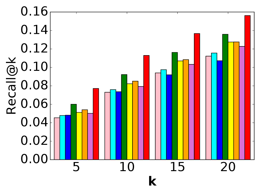

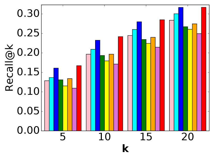


5.6. Performance Comparison
The performance comparison is shown in Figure 3 and Table 2. Based on these results, we have several observations.
Observations about our model. First, the proposed model, PMLAM, achieves the best performance on all five datasets with both evaluation metrics, which illustrates the superiority of our model.
Second, PMLAM outperforms SML. Although SML has an adaptive
margin mechanism, it is achieved by having a learnable scalar margin
for each user and item and adding a regularization term to prevent the learned
margins from being too small. It can be challenging to
identify an appropriate regularization weight via hyperparameter tuning.
By contrast, PMLAM formulates the adaptive margin generation
as a bilevel optimization, avoiding the additional
regularization. PMLAM employs a neural network to
generate the adaptive margin, so the number of parameters related to margin generation does not increase with the number of users or items.
Third, PMLAM achieves better performance than TransCF. One major reason is that TransCF only considers the items rated by a user and the users who rated an item as the neighbors of the user and item, respectively, which neglects the user-user/item-item relations. PMLAM models the user-user/item-item relations by two margin ranking losses with adaptive margins.
Fourth, PMLAM makes better recommendations than CML and LRML.
These methods apply a fixed margin for all user-item triplets and
do not measure or model the uncertainty of learned user/item
embeddings. PMLAM represents each user and item as a Gaussian
distribution, where the uncertainties of learned user preferences and
item properties are captured by the covariance matrices.
Fifth, PMLAM outperforms NCF and DeepAE. These are MLP-based
recommendation methods with the ability to capture non-linear
user-item relationships, but they violate the triangle inequality when modeling user-item interaction. As a result, they can struggle to capture the fine-grained user preference for particular items (Hsieh et al., 2017).
Other observations. First, all of the results reported
for the Comics dataset are
considerably better than those for the other datasets. The other four datasets are sparser and data sparsity negatively impacts recommendation performance.
Second, CML, LRML and TransCF perform better than SML on most of
the datasets. The adaptive margin regularization term in SML
struggles to adequately counterbalance SML’s tendency to
reduce the loss by imposing small margins. Although it is reported
that SML outperforms CML, LRML and TransCF
in (Li
et al., 2020), the experiments are conducted
on three relatively small-scale datasets with only several thousands
of users and items. We experiment with much larger datasets;
identifying a successful regularization setting appears to be more
difficult as the number of users increases.
Third, TransCF outperforms LRML on most of the datasets. One
possible reason is that TransCF has a more effective translation
embedding learning mechanism, which incorporates the neighborhood information of users and items. TransCF also has a regularization term to further pull positive items closer to the anchor user.
Fourth, CML achieves better performance than LRML on most of the
datasets. CML integrates the weighted
approximate-rank pairwise (WARP) weighting
scheme (Weston
et al., 2010) in the loss function to
penalize lower-ranked positive items. The comparison between CML and
LRML in (Tay et al., 2018) removes this component of CML.
The WARP scheme appears to play an important role in improving CML’s performance.
Fifth, DeepAE outperforms NCF. The heuristic weighting function
of DeepAE can impose useful penalties to errors that occur during training when positive items are assigned lower prediction scores.
| Architecture | CDs | Electronics \bigstrut | ||
|---|---|---|---|---|
| R@10 | N@10 | R@10 | N@10 \bigstrut | |
| (1) + Deter_Emb | 0.0721 | 0.0371 | 0.0241 | 0.0090 |
| (2) + Gauss_Emb | 0.0815 | 0.0434 | 0.0296 | 0.0110 |
| (3) + Deter_Emb | 0.0777 | 0.0415 | 0.0338 | 0.0125 |
| (4) - + Deter_Emb | 0.0408 | 0.0204 | 0.0139 | 0.0055 |
| (5) - + Deter_Emb | 0.0311 | 0.0158 | 0.0050 | 0.0018 |
| (6) + Gauss_Emb | 0.0856 | 0.0454 | 0.0365 | 0.0155 |
| (7) + + | 0.0966 | 0.0526 | 0.0429 | 0.0189 |
| (8) PMLAM | 0.1129 | 0.0619 | 0.0469 | 0.0234 |
5.7. Ablation Analysis
To verify and assess the relative effectiveness of the proposed user-item interaction module, the adaptive margin generation module, and the user-user/item-item relation module, we conduct an ablation study. Table 3 reports the performance improvement achieved by each module of the proposed model. Note that we compute Euclidean distances between deterministic embeddings. In (1), which serves as a baseline, we use the hinge loss with a fixed margin (Eq. 4) on deterministic embeddings of users and items to capture the user-item interaction ( is set to which is commonly used in (Hsieh et al., 2017; Tay et al., 2018; Park et al., 2018)). In (2), as an alternative baseline, we apply the same hinge loss as in (1), but replace the deterministic embeddings with parameterized Gaussian distributions (Section 4.1). In (3), we use the adaptive margin generation module (Section 4.2) to generate the margins for deterministic embeddings. In (4), we concatenate the deterministic embeddings of to generate instead of using Eq. 11. In (5), we sum the deterministic embeddings of to generate instead of using Eq. 11. In (6), we combine (2) and (3) to generate the adaptive margins for Gaussian embeddings. In (7), we augment (6) with user-user/item-item modeling but with a fixed margin, where the margin is also set to . In (8), we add the user-user/item-item modeling with adaptive margins (Section 4.3) to replace the fixed margins in the configuration of (7).
From the results in Table 3, we have several observations. First, from (1) and (2), we observe that by representing the user and item as Gaussian distributions and computing the distance between Gaussian distributions, the performance improves. This suggests that measuring the uncertainties of learned embeddings is significant. Second, from (1) and (3) along with (2) and (6), we observe that incorporating the adaptive margin generation module improves performance, irrespective of whether deterministic or Gaussian embeddings are used. These results demonstrate the effectiveness of the proposed margin generation module. Third, from (3), (4) and (5), we observe that our designed inputs (Eq. 11) for margin generation facilitate the production of appropriate margins compared to commonly used embedding concatenation or summation operations. Fourth, from (2), (3) and (6), we observe that (6) achieves better results than either (2) or (3), demonstrating that Gaussian embedddings and adaptive margin generation are compatible and can be combined to improve the model performance. Fifth, compared to (6), we observe that the inclusion of the user-user and item-item terms in the objective function (7) leads to a large improvement in recommendation performance. This demonstrates that explicit user-user/item-item modeling is essential and can be an effective supplement to infer user preferences. Sixth, from (7) and (8), we observe that adaptive margins also improve the modelling of the user-user/item-item relations.
| User | Positive | Sampled Movie | Margin |
|---|---|---|---|
| 405 | Scream (Thriller) | Four Rooms (Thriller) | 1.2752 |
| Toy Story (Animation) | 12.8004 | ||
| French Kiss (Comedy) | Addicted to Love (Comedy) | 2.6448 | |
| Batman (Action) | 12.4607 | ||
| 66 | Air Force One (Action) | GoldenEye (Action) | 0.3216 |
| Crumb (Documentary) | 5.0010 | ||
| The Godfather (Crime) | The Godfather II (Crime) | 0.0067 | |
| Terminator (Sci-Fi) | 3.6335 |
5.8. Case Study
In this section, we conduct case studies to confirm whether the adaptive margin generation can produce appropriate margins. To achieve this purpose, we train our model on the MovieLens-100K dataset. This dataset provides richer side information about movies (e.g., movie genres), making it easier for us to illustrate the results. Since we only focus on the adaptive margin generation, we use deterministic embeddings of users and items to avoid the interference of other modules. We randomly sample users from the dataset. For each user, we sample one item that the user has accessed as the positive item and two items the user did not access as negative items, where one item has a similar genre with the positive item and the other does not. The case study results are shown in Table 4.
As shown in Table 4, our adaptive margin generation module tends to generate a smaller margin value when the negative movie has a similar genre with the positive movie, while generating larger margins when they are distinct. The generated margins thus encourage the model to embed items with a higher probability of being preferred closer to the user’s embedding.
6. Conclusion
In this paper, we propose a distance-based recommendation model for top-K recommendation. Each user and item in our model are represented by Gaussian distributions with learnable parameters to handle the uncertainties. By incorporating an adaptive margin scheme, our model can generate fine-grained margins for the training triples during the training procedure. To explicitly capture the user-user/item-item relations, we adopt two margin ranking losses with adaptive margins to force similar user and item pairs to map closer together in the latent space. Experimental results on five real-world datasets validate the performance of our model, demonstrating improved performance compared to many state-of-the-art methods and highlighting the effectiveness of the Gaussian embeddings and the adaptive margin generation scheme. The code is available at https://github.com/huawei-noah/noah-research/tree/master/PMLAM.
References
- (1)
- Bordes et al. (2013) Antoine Bordes, Nicolas Usunier, Alberto García-Durán, Jason Weston, and Oksana Yakhnenko. 2013. Translating Embeddings for Modeling Multi-relational Data. In Advances in Neural Information Processing Systems.
- Casella and Berger (2002) George Casella and Roger L Berger. 2002. Statistical inference. Duxbury Pacific Grove, CA.
- Cho et al. (2011) Eunjoon Cho, Seth A. Myers, and Jure Leskovec. 2011. Friendship and mobility: user movement in location-based social networks. In Proc. ACM Conf. Knowledge Discovery and Data Mining.
- Colson et al. (2007) Benoît Colson, Patrice Marcotte, and Gilles Savard. 2007. An overview of bilevel optimization. Annals OR (2007).
- Covington et al. (2016) Paul Covington, Jay Adams, and Emre Sargin. 2016. Deep Neural Networks for YouTube Recommendations. In Proc. ACM Conf. Recommender Systems.
- Givens and Shortt (1984) Clark R. Givens and Rae Michael Shortt. 1984. A class of Wasserstein metrics for probability distributions. The Michigan Mathematical Journal (1984).
- Guo et al. (2017) Huifeng Guo, Ruiming Tang, Yunming Ye, Zhenguo Li, and Xiuqiang He. 2017. DeepFM: A Factorization-Machine based Neural Network for CTR Prediction. In Proc. Int. Joint Conf. Artificial Intelligence.
- He et al. (2017a) Ruining He, Wang-Cheng Kang, and Julian McAuley. 2017a. Translation-based Recommendation. In Proc. ACM Conf. Recommender Systems.
- He and McAuley (2016) Ruining He and Julian McAuley. 2016. Ups and Downs: Modeling the Visual Evolution of Fashion Trends with One-Class Collaborative Filtering. In Proc. Int. Conf. World Wide Web.
- He et al. (2017b) Xiangnan He, Lizi Liao, Hanwang Zhang, Liqiang Nie, Xia Hu, and Tat-Seng Chua. 2017b. Neural Collaborative Filtering. In Proc. Int. Conf. World Wide Web.
- He et al. (2016) Xiangnan He, Hanwang Zhang, Min-Yen Kan, and Tat-Seng Chua. 2016. Fast Matrix Factorization for Online Recommendation with Implicit Feedback. In Proc. ACM Int. Conf. Research and Development in Information Retrieval.
- Hsieh et al. (2017) Cheng-Kang Hsieh, Longqi Yang, Yin Cui, Tsung-Yi Lin, Serge J. Belongie, and Deborah Estrin. 2017. Collaborative Metric Learning. In Proc. Int. Conf. World Wide Web.
- Hu et al. (2008) Yifan Hu, Yehuda Koren, and Chris Volinsky. 2008. Collaborative Filtering for Implicit Feedback Datasets. In Proc. IEEE Int. Conf. Data Mining.
- Kabbur et al. (2013) Santosh Kabbur, Xia Ning, and George Karypis. 2013. FISM: factored item similarity models for top-N recommender systems. In Proc. ACM Conf. Knowledge Discovery and Data Mining.
- Kingma and Welling (2014) Diederik P. Kingma and Max Welling. 2014. Auto-Encoding Variational Bayes. In Proc. Int. Conf. Learning Representations.
- Koren et al. (2009) Yehuda Koren, Robert M. Bell, and Chris Volinsky. 2009. Matrix Factorization Techniques for Recommender Systems. IEEE Computer (2009).
- Li et al. (2020) Mingming Li, Shuai Zhang, Fuqing Zhu, Wanhui Qian, Liangjun Zang, Jizhong Han, and Songlin Hu. 2020. Symmetric Metric Learning with Adaptive Margin for Recommendation. (2020).
- Liu et al. (2019) Hanxiao Liu, Karen Simonyan, and Yiming Yang. 2019. DARTS: Differentiable Architecture Search. In Proc. Int. Conf. Learning Representations.
- Ma et al. (2019a) Chen Ma, Peng Kang, and Xue Liu. 2019a. Hierarchical Gating Networks for Sequential Recommendation. In Proc. ACM Conf. Knowledge Discovery and Data Mining.
- Ma et al. (2019b) Chen Ma, Peng Kang, Bin Wu, Qinglong Wang, and Xue Liu. 2019b. Gated Attentive-Autoencoder for Content-Aware Recommendation. In Proc. ACM Int. Conf. Web Search and Data Mining.
- Ma et al. (2020) Chen Ma, Liheng Ma, Yingxue Zhang, Jianing Sun, Xue Liu, and Mark Coates. 2020. Memory Augmented Graph Neural Networks for Sequential Recommendation. In AAAI.
- Ma et al. (2018) Chen Ma, Yingxue Zhang, Qinglong Wang, and Xue Liu. 2018. Point-of-Interest Recommendation: Exploiting Self-Attentive Autoencoders with Neighbor-Aware Influence. In Proc. ACM Int. Conf. Information and Knowledge Management.
- Mallasto and Feragen (2017) Anton Mallasto and Aasa Feragen. 2017. Learning from uncertain curves: The 2-Wasserstein metric for Gaussian processes. In Advances in Neural Information Processing Systems.
- Ning et al. (2015) Xia Ning, Christian Desrosiers, and George Karypis. 2015. A Comprehensive Survey of Neighborhood-Based Recommendation Methods. In Recommender Systems Handbook.
- Pan et al. (2008) Rong Pan, Yunhong Zhou, Bin Cao, Nathan Nan Liu, Rajan M. Lukose, Martin Scholz, and Qiang Yang. 2008. One-Class Collaborative Filtering. In Proc. IEEE Int. Conf. Data Mining.
- Park et al. (2018) Chanyoung Park, Donghyun Kim, Xing Xie, and Hwanjo Yu. 2018. Collaborative Translational Metric Learning. In Proc. IEEE Int. Conf. Data Mining.
- Rendle (2012) Steffen Rendle. 2012. Learning recommender systems with adaptive regularization. In Proc. ACM Int. Conf. Web Search and Data Mining.
- Rendle et al. (2009) Steffen Rendle, Christoph Freudenthaler, Zeno Gantner, and Lars Schmidt-Thieme. 2009. BPR: Bayesian Personalized Ranking from Implicit Feedback. In Proc. Conf. Uncertainty in Artificial Intelligence.
- Salakhutdinov and Mnih (2007) Ruslan Salakhutdinov and Andriy Mnih. 2007. Probabilistic Matrix Factorization. In Advances in Neural Information Processing Systems.
- Salakhutdinov et al. (2007) Ruslan Salakhutdinov, Andriy Mnih, and Geoffrey E. Hinton. 2007. Restricted Boltzmann machines for collaborative filtering. In Proc. Int. Conf. Machine Learning.
- Sarwar et al. (2001) Badrul Munir Sarwar, George Karypis, Joseph A. Konstan, and John Riedl. 2001. Item-based collaborative filtering recommendation algorithms. In Proc. Int. Conf. World Wide Web.
- Shrivastava and Li (2014) Anshumali Shrivastava and Ping Li. 2014. Asymmetric LSH (ALSH) for Sublinear Time Maximum Inner Product Search (MIPS). In Advances in Neural Information Processing Systems.
- Sinha et al. (2018) Ankur Sinha, Pekka Malo, and Kalyanmoy Deb. 2018. A Review on Bilevel Optimization: From Classical to Evolutionary Approaches and Applications. IEEE Trans. Evolutionary Computation (2018).
- Srivastava (2008) Sashi Mohan Srivastava. 2008. A course on Borel sets. Springer Science & Business Media.
- Sukhbaatar et al. (2015) Sainbayar Sukhbaatar, Arthur Szlam, Jason Weston, and Rob Fergus. 2015. End-To-End Memory Networks. In Advances in Neural Information Processing Systems.
- Sun et al. (2019) Jianing Sun, Yingxue Zhang, Chen Ma, Mark Coates, Huifeng Guo, Ruiming Tang, and Xiuqiang He. 2019. Multi-graph Convolution Collaborative Filtering. In Proc. IEEE Int. Conf. Data Mining.
- Tay et al. (2018) Yi Tay, Luu Anh Tuan, and Siu Cheung Hui. 2018. Latent Relational Metric Learning via Memory-based Attention for Collaborative Ranking. In Proc. Int. Conf. World Wide Web.
- Wan and McAuley (2018) Mengting Wan and Julian McAuley. 2018. Item recommendation on monotonic behavior chains. In Proc. ACM Conf. Recommender Systems.
- Wang et al. (2015) Hao Wang, Naiyan Wang, and Dit-Yan Yeung. 2015. Collaborative Deep Learning for Recommender Systems. In Proc. ACM Conf. Knowledge Discovery and Data Mining.
- Wang et al. (2019) Xiang Wang, Xiangnan He, Meng Wang, Fuli Feng, and Tat-Seng Chua. 2019. Neural Graph Collaborative Filtering. In Proc. ACM Int. Conf. Research and Development in Information Retrieval.
- Weston et al. (2010) Jason Weston, Samy Bengio, and Nicolas Usunier. 2010. Large scale image annotation: learning to rank with joint word-image embeddings. Machine Learning (2010).
- Wu et al. (2016) Yao Wu, Christopher DuBois, Alice X. Zheng, and Martin Ester. 2016. Collaborative Denoising Auto-Encoders for Top-N Recommender Systems. In Proc. ACM Int. Conf. Web Search and Data Mining.
- Xie et al. (2019) Yujia Xie, Xiangfeng Wang, Ruijia Wang, and Hongyuan Zha. 2019. A Fast Proximal Point Method for Computing Exact Wasserstein Distance. In Proc. Conf. Uncertainty in Artificial Intelligence.
- Xue et al. (2017) Hong-Jian Xue, Xinyu Dai, Jianbing Zhang, Shujian Huang, and Jiajun Chen. 2017. Deep Matrix Factorization Models for Recommender Systems. In Proc. Int. Joint Conf. Artificial Intelligence.