Probabilistic Guarantees of Stochastic Recursive Gradient in Non-Convex Finite Sum Problems

• •

  High-Probability Bounds: While most works in the literature of optimization provide in-expectation bounds, there is only a small fraction of works discussing bounds in the high probability sense. [17] provide a high-probability bound on the excess risk given a bound on the regret. [12], [8, 9] derive some high-probability bounds for SGD in convex online optimization problems. [34, 22] prove high-probability bounds for several adaptive methods, including AMSGrad, RMSProp and Delayed AdaGrad with momentum. All these works rely on (generalized) Freedman’s inequality or the concentration inequality given in Lemma 6 in [15]. Different from them, our high-probability results are built on a novel Azuma-Hoeffding type inequality proved in this work and Corollary 8 from [15]. In addition, we notice that [23] provide some probabilistic bounds on a SARAH-based algorithm. However, we believe their use of the plain martingale Azuma-Hoeffding inequality is not justifiable. [5] show in-probability upper bound for SPIDER. Nevertheless, SPIDER’s practical performance is inferior due to its accuracy-dependent small step size [32, 33].

• •

  Variance-Reduced Methods in Non-Convex Finite Sum Problems: Since the invention of the variance-reduction technique in [18, 16, 4], there has been a large amount of work incorporating this efficient technique to methods targeting the non-convex finite-sum problem. Subsequent methods, including SVRG ([1, 31, 25]), SARAH ([27, 28]), SCSG ([19, 21, 11]), SNVRG ([34]), SPIDER ([5]), SpiderBoost ([33]) and PAGE ([24]), have greatly reduced computational complexity in non-convex problems.

• •

  Dimension-Free Martingale Azuma-Hoeffding inequality: To facilitate our probabilistic analysis, we provide a novel Azuma-Hoeffding type bound on the summation norm of a martingale difference sequence. The novelty is two-fold. Firstly, same as the plain martingale Azuma-Hoeffding inequality, it provides a dimension-free bound. In a recent paper, a sub-Gaussian type bound has been developed by [15]. However, their results are not dimension-free. Our technique in the proof is built on a classic paper by [29] and is completely different from the random matrix technique used in [15]. Secondly, our concentration inequality allows random bounds on each element of the martingale difference sequence, which is much tighter than a large deterministic bound. It should be highlighted that our novel concentration result perfectly suits the nature of SARAH-style methods where the increment can be characterized as a martingale difference sequence and it can be further used to analyze other algorithms beyond the current paper.

• •

  In-probability error bounds of stochastic recursive gradient: We design a SARAH-based algorithm, named Prob-SARAH, adapted to the high-probability target and provably show its good in-probability properties. Under appropriate parameter setting, the first order complexity needed to achieve the in-probability target is $\tilde{\mathcal{O}}\left(\frac{1}{\varepsilon^{3}}\wedge\frac{\sqrt{n}}{\varepsilon^{2}}\right)$, which matches the best known in-expectation upper bound up to some logarithmic factors ([34, 33, 11]). We would like to point out that the parameter setting used to achieve such complexity is semi-adaptive to $\varepsilon$. That is, only the final stopping rule relies on $\varepsilon$ while other key parameters are independent of $\varepsilon$, including step size, mini-batch sizes, and lengths of loops.

• •

  Probabilistic analysis of SARAH for non-convex finite sum: Existing literature on the bounds of SARAH is mostly focusing on the strongly convex or general convex settings. We extend the case to the non-convex scenarios, which can be considered as a complimentary study to the stochastic recursive gradient in probability.

For a sequence of sets $\mathcal{A}_{1},\mathcal{A}_{2},\ldots$, we denote the smallest sigma algebra containing $\mathcal{A}_{i}$, $i\geq 1$, by $\sigma\big{(}\bigcup_{i=1}^{\infty}\mathcal{A}_{i}\big{)}$. By abuse of notation, for a random variable $\mathbf{X}$, we denote the sigma algebra generated by $\mathbf{X}$ by $\sigma(\mathbf{X})$. We define constant $C_{e}=\sum_{i=0}^{\infty}i^{-2}$. For two scalars $a,b\in\mathbb{R}$, we denote $a\wedge b=\min\{a,b\}$ and $a\vee b=\max\{a,b\}$. When we say a quantity $T$ is $\mathcal{O}_{\theta_{1},\theta_{2}}(\theta_{3})$ for some $\theta_{1},\theta_{2},\theta_{3}\in\mathbb{R}$, there exists a $g\in\mathbb{R}$ polylogarithmic in $\theta_{1}$ and $\theta_{2}$ such that $T\leq g\cdot\theta_{3}$, and similarly $\tilde{\mathcal{O}}_{(\cdot)}(\cdot)$ is defined the same but up to a logarithm factor.

We shall introduce some necessary regularized assumptions. Most assumptions are commonly used in the optimization literature. We have further clarifications in Appendix A.

Assumption 3.1 also indicates that there exists a positive number $\Delta_{f}$ such that $\sup_{\mathbf{x}\in\mathcal{D}}\big{[}f(\mathbf{x})-f(\mathbf{x}^{*})\big{]}\leq\Delta_{f}.$ Assumptions 3.1–3.3 are commonly used in the optimization literature, and Assumption 3.4 can be easily satisfied in practical use as long as the initial points are not too far from the optimum. See more comments on assumptions in Appendix A.

According to the definition given in [20], an algorithm is called $\varepsilon$-independent if it can guarantee convergence at all target accuracies $\varepsilon$ in expectation without explicitly using $\varepsilon$ in the algorithm. This is a very favorable property because it means that we no longer need to set the target error beforehand. Here, we introduce a similar property regarding the dependency on $\varepsilon$.

The newly introduced property can be perceived as the probabilistic equivalent of $\varepsilon$-independence. As stated in the succeeding theorem, under the given conditions, Prob-SARAH can achieve $\varepsilon$-semi-independence, given $\delta$.

More detailed results can be found in Appendix C. In appendix C, we also introduce another hyper-parameter setting that can lead to a complexity with better dependency on $\alpha_{M}^{2}$, which could be implicitly affected by the choice of constraint region $\mathcal{D}$.

In this part, we explain the idea of the proof of Theorem 3.1. Same proofing strategy can be applied to other hyper-parameter settings. First, we bound the difference between $\boldsymbol{\nu}_{k}^{(j)}$ and $\nabla f\big{(}\mathbf{x}_{k}^{(j)}\big{)}$ by a linear combination of $\{\|\boldsymbol{\nu}_{m}^{(j)}\|\}_{m=0}^{k-1}$ and small remainders, with which we can have a good control on $\|\nabla f\big{(}\mathbf{x}_{k}^{(j)}\big{)}\|$ when the stopping rules are met. Second, we bound the number of steps we need to meet the stopping rules. Combining these 2 key components, we can smoothly get the final conclusions.

Let us firstly introduce a novel Azuma-Hoeffding type inequality, which is key to our analysis.

The success of Algorithm 1 is largely because $\nabla f(\mathbf{x}_{k}^{(j)})$ is well-approximated by $\boldsymbol{\nu}_{k}^{(j)}$, and meanwhile $\boldsymbol{\nu}_{k}^{(j)}$ can be easily updated. We can observe that $\boldsymbol{\nu}_{k}^{(j)}-\nabla f(\mathbf{x}_{k}^{(j)})$ is actually sum of a sequence of martingale difference as

To be more specific, let $\mathcal{F}_{0}=\{\emptyset,\Omega\}$, and iteratively define $\mathcal{F}_{j,-1}=\mathcal{F}_{j-1}$, $\mathcal{F}_{j,0}=\sigma\big{(}\mathcal{F}_{j-1}\cup\sigma(\mathcal{I}_{j})\big{)}$, $\mathcal{F}_{j,k}=\sigma\big{(}\mathcal{F}_{j,0}\cup\sigma(\mathcal{I}_{k}^{(j)})\big{)}$, $\mathcal{F}_{j}=\sigma\big{(}\bigcup\limits_{k=1}\limits^{\infty}\mathcal{F}_{j,k}\big{)}$, $j\geq 1,k\geq 1$. We also denote $\boldsymbol{\epsilon}_{0}^{(j)}\triangleq\boldsymbol{\nu}_{0}^{(j)}-\nabla f\big{(}\mathbf{x}_{0}^{(j)}\big{)}$, $\boldsymbol{\epsilon}_{m}^{(j)}\triangleq\frac{1}{b_{j}}\sum\limits_{i\in\mathcal{I}_{m}^{(j)}}\nabla f_{i}(\mathbf{x}_{m}^{(j)})-\nabla f(\mathbf{x}_{m}^{(j)})+\nabla f(\mathbf{x}_{m-1}^{(j)})-\frac{1}{b_{j}}\sum\limits_{i\in\mathcal{I}_{m}^{(j)}}\nabla f_{i}(\mathbf{x}_{m-1}^{(j)})$, $m\geq 1$. Then, we can see that $\{\boldsymbol{\epsilon}_{m}^{(j)}\}_{m=0}^{k}$ is a martingale difference sequence adapted to $\{\mathcal{F}_{j,m}\}_{m=-1}^{k}$. With the help of our new Martingale Azuma-Hoeffding inequality, we can control the difference between $\boldsymbol{\nu}_{k}^{(j)}$ and $\nabla f\big{(}\mathbf{x}_{k}^{(j)}\big{)}$ by a linear combination of $\{\|\boldsymbol{\nu}_{m}^{(j)}\|\}_{m=0}^{k-1}$ and small remainders, with details given in Appendix D.1. Then, given the stopping rules in line 11 and selection method specified in line 12 of Algorithm 1, it would be not hard for us to obtain $\left\|\nabla f(\hat{\mathbf{x}})\right\|^{2}\leq\varepsilon^{2}$ with a high probability. More details can be found in Appendix D.2.

Another key question needed to be resolved is, when the algorithm can stop? The following analysis can build some intuitions for us. Given a $T\in\mathbb{Z}_{+}$, with the bound given in Proposition F.1 in Appendix F, with a high probability,

where $A_{T}$ is upper bounded by a value polylogorithmic in $T$. As for the second summation, if $\varepsilon_{j}\leq\frac{1}{2}\varepsilon^{2}$ for $j=T,T+1,\ldots,2T$ (which is obviously true when $T$ is moderately large) and our algorithm doesn’t stop in $2T$ outer iterations,

which grows at least linear in $T$. Consequently, when $T$ is sufficiently large, the RHS of (7) can be smaller than $-\Delta_{f}$, which leads to a contradiction. Roughly, we can see that the stopping time $T$ cannot exceed the order of $\tilde{\mathcal{O}}\big{(}\frac{1}{\varepsilon}\vee\frac{1}{\sqrt{n}\varepsilon^{2}}\big{)}$. More details can be found in Appendix D.3.

In this part, we consider to add a non-convex regularization term to the commonly-used logistic regression. Specifically, given a sequence of observations $(\mathbf{w}_{i},y_{i})\in\mathbb{R}^{d}\times\{-1,1\}$, $i=1,2,\ldots,n$ and a regularized parameter $\lambda>0$, the objective is

Such an objective has also been considered in other works like [11] and [14]. Same as other works, we set the regularized parameter $\lambda=0.1$ across all experiments. We compare the newly-introduced Prob-SARAH against three popular methods including SGD ([6]), SVRG ([31]) and SCSG ([21]). Based on results given in Theorem 3.1, we let the length of the inner loop $K_{j}\sim j\wedge\sqrt{n}$, the inner loop batch size $b_{j}\sim\log j\left(j\wedge\sqrt{n}\right)$, the outer loop batch size $B_{j}\sim j^{2}\wedge n$. For fair comparison, we determine the batch size (inner loop batch size) for SGD (SCSG and SVRG) based on the sample size $n$ and the number of epochs needed to have sufficient decrease in gradient norm. For example, for the w7a dataset, the sample size is 24692 and we run 60 epochs in total. In the 20th epoch, the inner loop batch size of Prob-SARAH is approximately $67\log 67\approx 281$. Thus, we set batch size 256 for SGD, SCSG and SVRG so that they can be roughly matched. In addition, based on the theoretical results from [31], we also consider a large inner loop batch size comparable to $n^{2/3}$ for SVRG. In addition, we set step size $\eta=0.01$ for all algorithms across all experiments for simplicity.

Results are displayed in Figure 2, from which we can see that Prob-SARAH has superior probabilistic guarantee in controlling the gradient norm in all experiments. It is significantly better than SCSG and SVRG under our current setting. Prob-SARAH can achieve a lower gradient norm than SGD at the early stage while SGD has a slight advantage when the number of epochs is large.

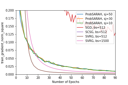
We also evaluate the performance of Prob-SARAH, SGD, SVRG and SCSG on the MNIST dataset with a simple 2-layer neural network. The two hidden layers respectively have 128 and 64 neurons. We include a GELU activation layer following each hidden layer. We use the negative log likelihood as our loss function. Under this setting, the objective is possibly non-convex and smooth on any given compact set. The step size is fixed to be 0.01 for all algorithms. For Prob-SARAH, we still have the length of the inner loop $K_{j}\sim j\wedge\sqrt{n}$, the inner loop batch size $b_{j}\sim\log j\left(j\wedge\sqrt{n}\right)$, the outer loop batch size $B_{j}\sim j^{2}\wedge n$. But to reduce computational time, we let $j$ start from 10, 30 and 50 respectively. Based on the same rule described in the previous subsection, we let the batch size (or inner loop batch size) for SGD, SVRG and SCSG be 512.

Results are given in Figure 1. In terms of gradient norm, Prob-SARAH has the best performance among algorithms considered here when the number of epochs is relatively small. With increasing number of epochs, SVRG tends to be better in finding first-order stationary points. However, based on the 3rd and 4th columns in Figure 1, SVRG apparently has an inferior performance on the validation set, which indicates that it could be trapped at local minima. In brief, Prob-SARAH achieves the best tradeoff between finding a first-order stationary point and generalization.

We also consider another set of experiments by replacing the GELU activation function with ReLU, resulting in a non-smooth objective. The results are shown in Appendix G, which resemble those in Figure 1 and the similar conclusions can be drawn.

References

- [1] Zeyuan Allen-Zhu and Elad Hazan “Variance reduction for faster non-convex optimization” In International conference on machine learning, 2016, pp. 699–707 PMLR
- [2] Rémi Bardenet and Odalric-Ambrym Maillard “Concentration inequalities for sampling without replacement” In Bernoulli 21.3 Bernoulli Society for Mathematical StatisticsProbability, 2015, pp. 1361–1385
- [3] Stéphane Boucheron, Gábor Lugosi and Pascal Massart “Concentration inequalities: A nonasymptotic theory of independence” Oxford university press, 2013
- [4] Aaron Defazio, Francis Bach and Simon Lacoste-Julien “SAGA: A fast incremental gradient method with support for non-strongly convex composite objectives” In Advances in neural information processing systems, 2014, pp. 1646–1654
- [5] Cong Fang, Chris Junchi Li, Zhouchen Lin and Tong Zhang “SPIDER: near-optimal non-convex optimization via stochastic path integrated differential estimator” In Proceedings of the 32nd International Conference on Neural Information Processing Systems, 2018, pp. 687–697
- [6] Saeed Ghadimi and Guanghui Lan “Stochastic first-and zeroth-order methods for nonconvex stochastic programming” In SIAM Journal on Optimization 23.4 SIAM, 2013, pp. 2341–2368
- [7] Ian Goodfellow, Yoshua Bengio and Aaron Courville “Deep learning” MIT press, 2016
- [8] Nicholas JA Harvey, Christopher Liaw, Yaniv Plan and Sikander Randhawa “Tight analyses for non-smooth stochastic gradient descent” In Conference on Learning Theory, 2019, pp. 1579–1613 PMLR
- [9] Nicholas JA Harvey, Christopher Liaw and Sikander Randhawa “Simple and optimal high-probability bounds for strongly-convex stochastic gradient descent” In arXiv preprint arXiv:1909.00843, 2019
- [10] Wassily Hoeffding “Probability Inequalities for Sums of Bounded Random Variables” In Journal of the American Statistical Association 58.301, 1963, pp. 13–30
- [11] Samuel Horváth, Lihua Lei, Peter Richtárik and Michael I Jordan “Adaptivity of stochastic gradient methods for nonconvex optimization” In arXiv preprint arXiv:2002.05359, 2020
- [12] Prateek Jain, Dheeraj Nagaraj and Praneeth Netrapalli “Making the last iterate of sgd information theoretically optimal” In Conference on Learning Theory, 2019, pp. 1752–1755 PMLR
- [13] Gareth James, Daniela Witten, Trevor Hastie and Robert Tibshirani “An introduction to statistical learning” Springer, 2013
- [14] Kaiyi Ji, Zhe Wang, Bowen Weng, Yi Zhou, Wei Zhang and Yingbin Liang “History-gradient aided batch size adaptation for variance reduced algorithms” In International Conference on Machine Learning, 2020, pp. 4762–4772 PMLR
- [15] Chi Jin, Praneeth Netrapalli, Rong Ge, Sham M Kakade and Michael I Jordan “A short note on concentration inequalities for random vectors with subgaussian norm” In arXiv preprint arXiv:1902.03736, 2019
- [16] Rie Johnson and Tong Zhang “Accelerating stochastic gradient descent using predictive variance reduction” In Advances in neural information processing systems 26, 2013, pp. 315–323
- [17] Sham M Kakade and Ambuj Tewari “On the generalization ability of online strongly convex programming algorithms” In Advances in Neural Information Processing Systems, 2009, pp. 801–808
- [18] Nicolas Le Roux, Mark Schmidt and Francis Bach “A stochastic gradient method with an exponential convergence rate for finite training sets” In Proceedings of the 25th International Conference on Neural Information Processing Systems-Volume 2, 2012, pp. 2663–2671
- [19] Lihua Lei and Michael Jordan “Less than a single pass: Stochastically controlled stochastic gradient” In Artificial Intelligence and Statistics, 2017, pp. 148–156 PMLR
- [20] Lihua Lei and Michael I Jordan “On the adaptivity of stochastic gradient-based optimization” In SIAM Journal on Optimization 30.2 SIAM, 2020, pp. 1473–1500
- [21] Lihua Lei, Cheng Ju, Jianbo Chen and Michael I Jordan “Non-convex finite-sum optimization via SCSG methods” In Proceedings of the 31st International Conference on Neural Information Processing Systems, 2017, pp. 2345–2355
- [22] Xiaoyu Li and Francesco Orabona “A high probability analysis of adaptive sgd with momentum” In arXiv preprint arXiv:2007.14294, 2020
- [23] Zhize Li “SSRGD: Simple Stochastic Recursive Gradient Descent for Escaping Saddle Points” In Advances in Neural Information Processing Systems 32, 2019, pp. 1523–1533
- [24] Zhize Li, Hongyan Bao, Xiangliang Zhang and Peter Richtárik “PAGE: A simple and optimal probabilistic gradient estimator for nonconvex optimization” In International Conference on Machine Learning, 2021, pp. 6286–6295 PMLR
- [25] Zhize Li and Jian Li “A simple proximal stochastic gradient method for nonsmooth nonconvex optimization” In Proceedings of the 32nd International Conference on Neural Information Processing Systems, 2018, pp. 5569–5579
- [26] Yurii Nesterov “Introductory lectures on convex optimization: A basic course” Springer Science & Business Media, 2003
- [27] L M Nguyen, Jie Liu, Katya Scheinberg and Martin Takáč “SARAH: A novel method for machine learning problems using stochastic recursive gradient” In International Conference on Machine Learning, 2017, pp. 2613–2621 PMLR
- [28] Lam M Nguyen, Jie Liu, Katya Scheinberg and Martin Takáč “Stochastic recursive gradient algorithm for nonconvex optimization” In arXiv preprint arXiv:1705.07261, 2017
- [29] Iosif Pinelis “An approach to inequalities for the distributions of infinite-dimensional martingales” In Probability in Banach Spaces, 8: Proceedings of the Eighth International Conference, 1992, pp. 128–134 Springer
- [30] Iosif Pinelis “Optimum bounds for the distributions of martingales in Banach spaces” In The Annals of Probability JSTOR, 1994, pp. 1679–1706
- [31] Sashank J Reddi, Ahmed Hefny, Suvrit Sra, Barnabas Poczos and Alex Smola “Stochastic variance reduction for nonconvex optimization” In International conference on machine learning, 2016, pp. 314–323 PMLR
- [32] Quoc Tran-Dinh, Nhan H Pham, Dzung T Phan and Lam M Nguyen “Hybrid stochastic gradient descent algorithms for stochastic nonconvex optimization” In arXiv preprint arXiv:1905.05920, 2019
- [33] Zhe Wang, Kaiyi Ji, Yi Zhou, Yingbin Liang and Vahid Tarokh “Spiderboost and momentum: Faster variance reduction algorithms” In Advances in Neural Information Processing Systems 32, 2019, pp. 2406–2416
- [34] Dongruo Zhou, Jinghui Chen, Yuan Cao, Yiqi Tang, Ziyan Yang and Quanquan Gu “On the convergence of adaptive gradient methods for nonconvex optimization” In arXiv preprint arXiv:1808.05671, 2018