Private Inputs for Leader-Follower Game with Feedback Stackelberg Strategy

Yue Sun, Hongdan Li and Huanshui Zhang This work was supported by the National Natural Science Foundation of China under Grants 61821004 and the Natural Science Foundation of Shandong Province (ZR2021ZD14, ZR2021JQ24), and Science and Technology Project of Qingdao West Coast New Area (2019-32, 2020-20, 2020-1-4), High-level Talent Team Project of Qingdao West Coast New Area (RCTD-JC-2019-05), Key Research and Development Program of Shandong Province (2020CXGC01208). *Corresponding author.Y. Sun is with the School of Control Science and Engineering, Shandong University, Jinan, Shandong 250061, China (e-mail: [email protected]). H. Li and H. Zhang are with College of Electrical Engineering and Automation, Shandong University of Science and Technology, Qingdao, Shandong 266590, China (e-mail: [email protected]; [email protected]).

Abstract

In this paper, the two-player leader-follower game with private inputs for feedback Stackelberg strategy is considered. In particular, the follower shares its measurement information with the leader except its historical control inputs while the leader shares none of the historical control inputs and the measurement information with the follower. The private inputs of the leader and the follower lead to the main obstacle, which causes the fact that the estimation gain and the control gain are related with each other, resulting that the forward and backward Riccati equations are coupled and making the calculation complicated. By introducing a kind of novel observers through the information structure for the follower and the leader, respectively, a kind of new observer-feedback Stacklberg strategy is designed. Accordingly, the above-mentioned obstacle is also avoided. Moreover, it is found that the cost functions under the presented observer-feedback Stackelberg strategy are asymptotically optimal to the cost functions under the optimal feedback Stackelberg strategy with the feedback form of the state. Finally, a numerical example is given to show the efficiency of this paper.

Index Terms:

feedback Stackelberg strategy, private inputs, observers, asymptotic optimality.

I Introduction

In the traditional control model, centralized control is a basic concept and has been extensively studied from time-invariant system to time-variant system and system with time-delay [1, 2, 3]. However, with the development of wireless sensor network and artificial intelligence, the centralized control will no longer be applicable due to the fact that the achievable bandwidth would be limited by long delays induced by the communication between the centralized controller [4]. The task of effectively controlling multiple decision-makers systems in the absence of communication channels is increasingly an interesting and challenging control problem. Correspondingly, the decentralized control of large-scale systems arises accordingly, which has widespread implementation in electrical power distribution networks, cloud environments, multi-agent systems, reinforcement learning and so on [5, 6, 7, 8], where decisions are made by multiple different decision-makers who have access to different information.

Decentralized control can be traced back to 1970s [9, 10, 11]. The optimization of decentralized control can be divided into two categories. The first category is the decentralized control for multi-controllers with one associated cost function [12, 13, 14]. Nayyar studied decentralized stochastic control with partial history observations and control inputs sharing in [15] by using the common information approach and the $n$ -step delayed sharing information structure was investigated in [16]. [17] focused on decentralized control in networked control system with asymmetric information by solving the forward and backward coupled Riccati equations through forward iteration, where the historical control inputs was shared unilaterally compared with the information structure shared with each other in [15, 16]. [18] designed decentralized strategies for mean-field system, which was further shown to have asymptotic robust social optimality. The other category is the decentralized control for game theory [23, 24, 25]. Two-criteria LQG decision problems with one-step delay observation sharing pattern for stochastic discrete-time system in Stackelberg strategy and Nash equilibrium strategy were considered in [19] and [20], respectively. Necessary conditions for an optimal Stackelberg strategy with output feedback form were given in [21] with incomplete information of the controllers. [22] investigated feedback risk-sensitive Nash equilibrium solutions for two-player nonzero-sum games with complete state observation and shared historical control inputs. Static output feedback incentive Stackelberg game with markov jump for linear stochastic systems was taken into consideration in [26] and a numerical algorithm was further proposed which guaranteed local convergence.

Noting that the information structure in the decentralized control systems mentioned above has the following feature, that is, all or part of historical control inputs of the controllers are shared with the other controllers. However, the case, where the controllers have its own private control inputs, has not been addressed in decentralized control system, which has applications in a personalized healthcare setting, in the states of a virtual keyboard user (e.g., Google GBoard users) and in the social robot for second language education of children [27]. It should be noted that the information structure where the control information are unavailable to the other decision makers will cause the estimation gain depends on the control gain and vice versa, which means the forward and backward Riccati equations are coupled, and make the calculation more complicated. Motivated by [28], which focused on the LQ optimal control problem of linear systems with private input and measurement information by using a kind of novel observers to overcome the obstacle, in this paper, we are concerned with the feedback Stackelberg strategy for two-player game with private control inputs. In particular, the follower shares its measurement information to the leader, while the leader doesn’t share any information to the follower due to the hierarchical relationship and the historical control inputs for the follower and the leader are both private, which is the main obstacle in this paper. To overcome the problem, firstly, the novel observers based on the information structure of each controller are proposed. Accordingly, a new kind of observer-feedback Stackelberg strategy for the follower and the leader is designed. Finally, it proved that the associated cost functions for the follower and the leader under the proposed observer-feedback Stackelberg strategy are asymptotically optimal as compared with the cost functions under the optimal feedback Stackelberg strategy with the feedback form of the state obtained in [29].

The outline of this paper is given as follows. The problem formulation is given in Section II. The observers and the observer-feedback Stackelberg strategy with private inputs are designed in Section III. The asymptotical optimal analysis is shown in Section IV. Numerical examples are presented in Section V. Conclusion is given in Section VI.

Notations: $\mathbb{R}^{n}$ represents the space of all real $n$ -dimensional vectors. $A^{\prime}$ means the transpose of the matrix $A$ . A symmetric matrix $A>0$ (or $A\geq 0$ ) represents that the matrix $A$ is positive definite (or positive semi-definite). $\|x\|$ denotes the Euclidean norm of vector $x$ , i.e., $\|x\|^{2}=x^{\prime}x$ . $\|A\|$ denotes the Euclidean norm of matrix $A$ , i.e., $\|A\|=\sqrt{\lambda_{max}(A^{\prime}A)}$ . $\lambda(A)$ represents the eigenvalues of the matrix $A$ and $\lambda_{max}(A)$ represents the largest eigenvalues of the matrix $A$ . $I$ is an identity matrix with compatible dimension. $0$ in block matrix represents a zero matrix with appropriate dimensions.

II Problem Formulation

Consider a two-player leader-follower game described as:

$\displaystyle x(k+1)$	$\displaystyle=$	$\displaystyle Ax(k)+B_{1}u_{1}(k)+B_{2}u_{2}(k),$	(1)
$\displaystyle y_{1}(k)$	$\displaystyle=$	$\displaystyle H_{1}x(k),$	(2)
$\displaystyle y_{2}(k)$	$\displaystyle=$	$\displaystyle H_{2}x(k),$	(3)

where $x(k)\in\mathbb{R}^{n}$ is the state with initial value $x(0)$ . $u_{1}(k)\in\mathbb{R}^{m_{1}}$ and $u_{2}(k)\in\mathbb{R}^{m_{2}}$ are the two control inputs of the follower and the leader, respectively. $y_{i}(k)\in\mathbb{R}^{s_{i}}$ is the measurement information. $A$ , $B_{i}$ and $H_{i}$ ( $i=1,2$ ) are constant matrices with compatible dimensions.

The associated cost functions for the follower and the leader are given by

$\displaystyle J_{1}$	$\displaystyle=$	$\displaystyle\sum\limits^{\infty}_{k=0}[x^{\prime}(k)Q_{1}x(k)+u^{\prime}_{1}(k)R_{11}u_{1}(k)$	(4)
		$\displaystyle+u^{\prime}_{2}(k)R_{12}u_{2}(k)],$	(4)
$\displaystyle J_{2}$	$\displaystyle=$	$\displaystyle\sum\limits^{\infty}_{k=0}[x^{\prime}(k)Q_{2}x(k)+u^{\prime}_{1}(k)R_{21}u_{1}(k)$	(5)
		$\displaystyle+u^{\prime}_{2}(k)R_{22}u_{2}(k)],$	(5)

where the weight matrices are such that $Q_{i}\geq 0$ , $R_{ij}\geq 0$ ( $i\neq j$ ) and $R_{ii}>0$ ( $i,j=1,2$ ) with compatible dimensions.

Feedback Stackelberg strategy with different information structure for controllers had been considered since 1970s in [29], where the information structure satisfied that the controller shared all or part of historical inputs to the other. To the best of our knowledge, there has been no efficiency technique to deal with the case of private inputs for controllers. The difficultly lies in the unavailability of other controllers’ historical control inputs, which leads to the fact that the estimation gain depends on the control gain and makes the forward and backward Riccati equations coupled. In this paper, our goal is that by designing the novel observers based on the measurements and private inputs for the follower and the leader, respectively, we will show the proposed observer-feedback Stackelberg strategy is asymptotic optimal to the deterministic case in [29]. Mathematically, by denoting

$\displaystyle Y_{i}(k)$	$\displaystyle=$	$\displaystyle\{y_{i}(0),...,y_{i}(k)\},$
$\displaystyle U_{i}(k-1)$	$\displaystyle=$	$\displaystyle\{u_{i}(0),...,u_{i}(k-1)\},$
$\displaystyle{F}_{1}(k)$	$\displaystyle=$	$\displaystyle\{Y_{1}(k),U_{1}(k-1)\},$	(6)
$\displaystyle{F}_{2}(k)$	$\displaystyle=$	$\displaystyle\{Y_{1}(k),Y_{2}(k),U_{2}(k-1)\},$	(7)

we will design the observer-feedback Stackelberg strategy based on the information $\mathcal{F}_{i}(k)$ , where $u_{i}(k)$ is $\mathcal{F}_{i}(k)$ -casual for $i=1,2$ in this paper. The following assumptions will be used in this paper.

Assumption 1

System $(A,B)$ is stabilizable with $B=\left[\begin{array}[]{cc}B_{1}&B_{2}\\ \end{array}\right]$ and system $(A,Q_{i})$ ( $i=1,2$ ) is observable.

By denoting the admissible controls sets $\mathcal{U}_{i}$ (i=1, 2) for the feedback Stackelberg strategy of the follower and the leader:

	$\displaystyle\mathcal{U}_{1}$	$\displaystyle=\{$	$\displaystyle u_{1}:\Omega\times[0,N]\times\mathbb{R}^{n}\times U_{2}\longrightarrow U_{1}\},$
	$\displaystyle\mathcal{U}_{2}$	$\displaystyle=\{$	$\displaystyle u_{2}:\Omega\times[0,N]\times\mathbb{R}^{n}\longrightarrow U_{2}\},$		(8)

where $U_{1}$ and $U_{2}$ represent the strategy for the follower and the leader, respectively, the definition of the feedback Stackelberg strategy [30] is given.

Definition 1

$(u^{*}_{1}(k),u^{*}_{2}(k))\in\mathcal{U}_{1}\times\mathcal{U}_{2}$ is the optimal feedback Stackelberg strategy, if there holds that:

	$\displaystyle J_{1}(u^{}_{1}(k,u^{}_{2}(k)),u^{*}_{2}(k))$	$\displaystyle\leq$	$\displaystyle J_{1}(u_{1}(k,u^{}_{2}(k)),u^{}_{2}(k)),\forall u_{1}\in\mathcal{U}_{1},$
	$\displaystyle J_{2}(u^{}_{1}(k,u^{}_{2}(k)),u^{*}_{2}(k))$	$\displaystyle\leq$	$\displaystyle J_{2}(u^{*}_{1}(k,u_{2}(k)),u_{2}(k)),\forall u_{2}\in\mathcal{U}_{2}.$

Firstly, the optimal feedback Stackelberg strategy in deterministic case with perfect information structure is given, that is, the information structure of the follower and the leader both satisfy

\displaystyle Y_{k}=\{x(0),...,x(k),u_{i}(0),...,u_{i}(k-1),\quad i=1,2\}.

Lemma 1

Under Assumption 1, the optimal feedback Stackelberg strategy with the information structure for the follower and the leader satisfying $Y_{k}$ , is given by

	$\displaystyle u_{1}(k)$	$\displaystyle=$	$\displaystyle K_{1}x(k),$		(9)
	$\displaystyle u_{2}(k)$	$\displaystyle=$	$\displaystyle K_{2}x(k),$		(10)

where the feedback gain matrices $K_{1}$ and $K_{2}$ satisfy

	$\displaystyle K_{1}$	$\displaystyle=$	$\displaystyle-\Gamma^{-1}_{1}Y_{1},$		(11)
	$\displaystyle K_{2}$	$\displaystyle=$	$\displaystyle-\Gamma^{-1}_{2}Y_{2},$		(12)

with

$\displaystyle\Gamma_{1}$	$\displaystyle=$	$\displaystyle R_{11}+B^{\prime}_{1}P_{1}B_{1},$
$\displaystyle\Gamma_{2}$	$\displaystyle=$	$\displaystyle R_{22}+B^{\prime}_{2}M^{\prime}_{1}P_{2}M_{1}B_{2}+B^{\prime}_{2}S^{\prime}R_{21}SB_{2},$
$\displaystyle M_{1}$	$\displaystyle=$	$\displaystyle I-B_{1}S,\quad S=\Gamma^{-1}_{1}B^{\prime}_{1}P_{1},$
$\displaystyle Y_{1}$	$\displaystyle=$	$\displaystyle B^{\prime}_{1}P_{1}A+B^{\prime}_{1}P_{1}B_{2}K_{2},$
$\displaystyle Y_{2}$	$\displaystyle=$	$\displaystyle B^{\prime}_{2}M^{\prime}_{1}P_{2}M_{1}A+B^{\prime}_{2}S^{\prime}R_{21}SA,$

where $P_{1}$ and $P_{2}$ satisfy the following two-coupled algebraic Riccati equations:

$\displaystyle P_{1}$	$\displaystyle=$	$\displaystyle Q_{1}+(A+B_{2}K_{2})^{\prime}P_{1}(A+B_{2}K_{2})$	(13)
		$\displaystyle-Y^{\prime}_{1}\Gamma^{-1}_{1}Y_{1}+K^{\prime}_{2}R_{12}K_{2},$	(13)
$\displaystyle P_{2}$	$\displaystyle=$	$\displaystyle Q_{2}+A^{\prime}M^{\prime}_{1}P_{2}M_{1}A+A^{\prime}S^{\prime}R_{21}SA$	(14)
		$\displaystyle-Y^{\prime}_{2}\Gamma^{-1}_{2}Y_{2}.$	(14)

The optimal cost functions for feedback Stackelberg strategy are such that

	$\displaystyle J^{*}_{1}$	$\displaystyle=$	$\displaystyle x^{\prime}(0)P_{1}x(0),$		(15)
	$\displaystyle J^{*}_{2}$	$\displaystyle=$	$\displaystyle x^{\prime}(0)P_{2}x(0).$		(16)

Proof 1

The optimal feedback Stackelberg strategy for deterministic case with perfect information structure for the follower and the leader in finite-time horizon has been shown in (18)-(28) with $\theta(t)=\Pi_{1}(t)=\Pi_{2}(t)=0$ in [29]. By using the results in Theorem 2 in [3], the results obtained in [29] can be extended into infinite horizon, i.e., (18)-(28) in [29] are convergent to the algebraic equations obtained in (11)-(12) and (13)-(14) in Lemma 1 of this paper by using the monotonic boundedness theorem. This completes the proof.

Remark 1

$P_{1}>0$ and $P_{2}>0$ in (13)-(14) can be shown accordingly by using Theorem 2 in [3], which guaranteed the invertibility of $\Gamma_{1}$ and $\Gamma_{2}$ .

Remark 2

Compared with [29], where the historical control inputs of the follower and the leader are shared with each other, the historical control inputs of this paper are private, leading to the main obstacle.

III The observer-feedback Stackelberg strategy

Based on the discussion above, we are in position to consider the leader-follower game with private inputs, i.e., ${u}_{i}(k)$ is ${F}_{i}(k)$ -casual.

Remark 3

As pointed out in [17], the information structure in decentralized control, where one of the controllers (C1) doesn’t share the historical control inputs to the other controller (C2) while C2 shares its historical control inputs with C1, is a challenge problem due to the control gain and estimator gain are coupled. The difficulty with private inputs for the follower and the leader is even more complicated due to the unavailability of the historical control inputs of each controller.

Considering the private inputs of the follower and the leader, the observers $\hat{x}_{i}(k)$ ( $i=1,2$ ) are designed as follows:

$\displaystyle\hat{x}_{1}(k+1)$	$\displaystyle=$	$\displaystyle A\hat{x}_{1}(k)+B_{1}u^{\star}_{1}(k)+B_{2}K_{2}\hat{x}_{1}(k)$	(17)
		$\displaystyle+L_{1}[y_{1}(k)-H_{1}\hat{x}_{1}(k)],$	(17)
$\displaystyle\hat{x}_{2}(k+1)$	$\displaystyle=$	$\displaystyle A\hat{x}_{2}(k)+B_{1}K_{1}\hat{x}_{2}(k)+B_{2}u^{\star}_{2}(k)$	(18)
		$\displaystyle+L_{2}[y_{2}(k)-H_{2}\hat{x}_{2}(k)],$	(18)

where the observer gain matrices $L_{1}$ and $L_{2}$ are chosen to make the observers stable. Accordingly, the observer-feedback Stackelberg strategy is designed as follows:

	$\displaystyle u^{\star}_{1}(k)$	$\displaystyle=$	$\displaystyle K_{1}\hat{x}_{1}(k),$		(19)
	$\displaystyle u^{\star}_{2}(k)$	$\displaystyle=$	$\displaystyle K_{2}\hat{x}_{2}(k),$		(20)

where $K_{1}$ and $K_{2}$ are given in (11)-(12), respectively.

For convenience of future discussion, some symbols will be given beforehand.

$\displaystyle\mathcal{A}$	$\displaystyle=$	$\displaystyle\left[\begin{array}[]{cc}A+B_{2}K_{2}-L_{1}H_{1}&-B_{2}K_{2}\\ -B_{1}K_{1}&A+B_{1}K_{1}-L_{2}H_{2}\\ \end{array}\right],$	(23)
$\displaystyle\mathcal{B}$	$\displaystyle=$	$\displaystyle\left[\begin{array}[]{cc}-B_{1}K_{1}&-B_{2}K_{2}\\ \end{array}\right]$	(25)
	$\displaystyle=$	$\displaystyle\left[\begin{array}[]{cc}B_{1}S(A+B_{2}K_{2})&-B_{2}K_{2}\\ \end{array}\right],$	(27)
$\displaystyle\bar{A}$	$\displaystyle=$	$\displaystyle\left[\begin{array}[]{cc}A+B_{1}K_{1}+B_{2}K_{2}&\mathcal{B}\\ 0&\mathcal{A}\\ \end{array}\right],$	(30)
$\displaystyle\tilde{x}(k)$	$\displaystyle=$	$\displaystyle\left[\begin{array}[]{cc}\tilde{x}^{\prime}_{1}(k)&\tilde{x}^{\prime}_{2}(k)\\ \end{array}\right]^{\prime},$	(32)
$\displaystyle\tilde{x}_{i}(k)$	$\displaystyle=$	$\displaystyle x(k)-\hat{x}_{i}(k),\quad i=1,2.$

Subsequently, the stability of the observers $\hat{x}_{i}(k)$ ( $i=1,2$ ) and the stability of the closed-loop system (1) under the designed observer-feedback Stackelberg strategy (19)-(20) are shown, respectively.

Theorem 1

If there exist optional gain matrices $L_{1}$ and $L_{2}$ such that the matrix $\mathcal{A}$ is stable, then, the observers $\hat{x}_{i}(k)$ for $i=1,2$ are stable with the controllers of the follower and the leader satisfying (19)-(20), i.e., there holds

\displaystyle\lim_{k\rightarrow\infty}\|x(k)-\hat{x}_{i}(k)\|=0.

(33)

Proof 2

By substituting the observer-feedback controllers (19)-(20) into (1), then $x(k+1)$ is recalculated as:

$\displaystyle x(k+1)$	$\displaystyle=$	$\displaystyle Ax(k)+B_{1}K_{1}\hat{x}_{1}(k)+B_{2}K_{2}\hat{x}_{(}k)$	(34)
	$\displaystyle=$	$\displaystyle[A+B_{1}K_{1}+B_{2}K_{2}]x(k)-B_{1}K_{1}\tilde{x}_{1}(k)$
		$\displaystyle-B_{2}K_{2}\tilde{x}_{2}(k).$

Accordingly, by adding (19)-(20) into the observers (17)-(18) and combining with (34), the derivation of $\tilde{x}_{i}(k)$ for $i=1,2$ are given as

	$\displaystyle\tilde{x}_{1}(k+1)$	$\displaystyle=$	$\displaystyle(A+B_{2}K_{2}-L_{1}H_{1})\tilde{x}_{1}(k)-B_{2}K_{2}\tilde{x}_{2}(k),$
	$\displaystyle\tilde{x}_{2}(k+1)$	$\displaystyle=$	$\displaystyle(A+B_{1}K_{1}-L_{2}H_{2})\tilde{x}_{1}(k)-B_{1}K_{1}\tilde{x}_{1}(k),$

that is

\displaystyle\tilde{x}(k+1)

\displaystyle=

\displaystyle\mathcal{A}\tilde{x}(k).

(35)

Subsequently, if there exist matrices $L_{1}$ and $L_{2}$ making $\mathcal{A}$ stable, then, the stability of the matrix $\mathcal{A}$ means that

\displaystyle\lim_{k\rightarrow\infty}\tilde{x}(k)=0,

i.e., (33) is established. That is to say, the observers $\hat{x}_{i}(k)$ are stable under (19)-(20). The proof is completed.

Remark 4

Noting that in Theorem 1 the key point lies in that how to select $L_{i}$ ( $i=1,2$ ) so that the eigenvalues of the matrix $\mathcal{A}$ are within the unit circle. The following analysis gives an method to find $L_{i}$ .

According to the Lyapunov stability criterion, i.e., $\mathcal{A}$ is stable if and only if for any positive definite matrix $Q$ , $\mathcal{A}^{\prime}P\mathcal{A}-P=-Q$ admits a solution such that $P>0$ . Thus, if there exists a $P>0$ such that

\displaystyle\mathcal{A}^{\prime}P\mathcal{A}-P<0,

(36)

then $\mathcal{A}$ is stable. Following from the elementary row transformation, one has

	$\displaystyle\left(\begin{array}[]{cc}I&I\\ 0&I\\ \end{array}\right)\left(\begin{array}[]{cc}I&0\\ 0&\mathcal{A}^{\prime}\\ \end{array}\right)\left(\begin{array}[]{cc}-P&\mathcal{A}^{\prime}P\\ P\mathcal{A}&-P\\ \end{array}\right)\left(\begin{array}[]{cc}I&0\\ 0&\mathcal{A}\\ \end{array}\right)$
	$\displaystyle\times\left(\begin{array}[]{cc}I&0\\ I&I\\ \end{array}\right)=\left(\begin{array}[]{cc}\mathcal{A}^{\prime}P\mathcal{A}-P&0\\ 0&-\mathcal{A}^{\prime}P\mathcal{A}\\ \end{array}\right)<0,$

that is, $\mathcal{A}^{\prime}P\mathcal{A}-P<0$ is equivalent to the following matrix inequality

\displaystyle\left(\begin{array}[]{cc}-P&\mathcal{A}^{\prime}P\\ P\mathcal{A}&-P\\ \end{array}\right)<0.

(41)

Noting that $\mathcal{A}$ is related with $L_{i}$ , in order to use the linear matrix inequality (LMI) Toolbox in Matlab to find $L_{i}$ , (41) will be transmit into a LMI form. Let

\displaystyle P=\left(\begin{array}[]{cc}P&0\\ 0&P\\ \end{array}\right),\quad\tilde{W}=\left(\begin{array}[]{cc}W_{1}&0\\ 0&W_{2}\\ \end{array}\right),

and rewrite $\mathcal{A}$ in (23) as $\mathcal{A}=\tilde{A}-\tilde{L}\tilde{H}$ , where

	$\displaystyle\mathcal{A}$	$\displaystyle=$	$\displaystyle\left(\begin{array}[]{cc}A+B_{2}K_{2}&-B_{2}K_{2}\\ -B_{1}K_{1}&A+B_{1}K_{1}\\ \end{array}\right),$
	$\displaystyle\tilde{L}$	$\displaystyle=$	$\displaystyle\left(\begin{array}[]{cc}L_{1}&0\\ 0&L_{2}\\ \end{array}\right),\quad\tilde{H}=\left(\begin{array}[]{cc}H_{1}&0\\ 0&H_{2}\\ \end{array}\right).$

To this end, we have

\displaystyle P\mathcal{A}=P\tilde{A}-P\tilde{L}\tilde{H}=P\tilde{A}-\tilde{W}\tilde{H},

with $\tilde{W}=P\tilde{L}$ . Based on the discussion above, it concludes that $\mathcal{A}$ is stable if there exists a $P>0$ such that the following LMI:

\displaystyle\left(\begin{array}[]{cc}-P&(P\tilde{A}-\tilde{W}\tilde{H})^{\prime}\\ P\tilde{A}-\tilde{W}\tilde{H}&-P\\ \end{array}\right)<0.

(47)

In this way, by using the LMI Toolbox in Matlab, $L_{i}$ can be found according, which stabilizes $\mathcal{A}$ where $L_{i}=P^{-1}W_{i}$ .

Under the observer-feedback controllers (19)-(20), the stability of (1) is given.

Theorem 2

Under Assumption 1 and if there exists $L_{i}$ stabilizing $\mathcal{A}$ , then the closed-loop system (1) is stable with the observer-feedback controllers (19)-(20).

Proof 3

According to (34), the closed-loop system (1) is reformulated as

\displaystyle x(k+1)

\displaystyle=

\displaystyle[A+B_{1}K_{1}+B_{2}K_{2}]x(k)+\mathcal{B}\tilde{x}(k).

(48)

Together with (35), we have

\displaystyle\left[\begin{array}[]{c}x(k+1)\\ \tilde{x}(k+1)\\ \end{array}\right]

\displaystyle=

\displaystyle\bar{A}\left[\begin{array}[]{c}x(k)\\ \tilde{x}(k)\\ \end{array}\right].

(53)

The stability of $A+B_{1}K_{1}+B_{2}K_{2}$ is guaranteed by the stabilizability of $(A,B)$ and the observability of $(A,Q_{i})$ for $i=1,2$ . Following from Theorem 1, $\mathcal{A}$ is stabilized by selecting appropriate gain matrices $L_{1}$ and $L_{2}$ . Subsequently, the stability of the closed-loop system (1) is derived. This completes the proof.

IV The asymptotical optimal analysis

The stability of the state and the observers, i.e., $x(k)$ and $\hat{x}_{i}$ for $i=1,2$ has been shown in Theorem 1 and Theorem 2 under the observer-feedback controllers (19)-(20). To shown the rationality of the design of the observer-feedback controllers (19)-(20), the asymptotical optimal analysis relating with the cost functions under (19)-(20) is given. To this end, denote the cost functions for the follower and the leader satisfying

$\displaystyle J_{1}(s,M)$	$\displaystyle=$	$\displaystyle\sum\limits^{M}_{k=s}[x^{\prime}(k)Q_{1}x(k)+u^{\prime}_{1}(k)R_{11}u_{1}(k)$	(54)
		$\displaystyle+u^{\prime}_{2}(k)R_{12}u_{2}(k)],$	(54)
$\displaystyle J_{2}(s,M)$	$\displaystyle=$	$\displaystyle\sum\limits^{M}_{k=s}[x^{\prime}(k)Q_{2}x(k)+u^{\prime}_{1}(k)R_{21}u_{1}(k)$	(55)
		$\displaystyle+u^{\prime}_{2}(k)R_{22}u_{2}(k)].$	(55)

Now, we are in position to show that the observer-feedback Stackelberg strategy (19)-(20) is asymptotical optimal to the optimal feedback Stackelberg strategy presented in Lemma 1.

Theorem 3

Under Assumption 1, the corresponding cost functions (54)-(55) under the observer-feedback Stackelberg strategy (19)-(20) with $L_{i}$ ( $i=1,2$ ) selected from Theorem 1 are given by

$\displaystyle J^{\star}_{1}(s,\infty)$	$\displaystyle=$	$\displaystyle x^{\prime}(s)P_{1}x(s)$	(62)
		$\displaystyle+\sum\limits^{\infty}_{k=s}\left[\begin{array}[]{c}x(k)\\ \tilde{x}(k)\\ \end{array}\right]^{\prime}\left[\begin{array}[]{cc}0&T_{1}\\ T^{\prime}_{1}&S_{1}\\ \end{array}\right]\left[\begin{array}[]{c}x(k)\\ \tilde{x}(k)\\ \end{array}\right],$	(62)
$\displaystyle J^{\star}_{2}(s,\infty)$	$\displaystyle=$	$\displaystyle x^{\prime}(s)P_{2}x(s)$	(69)
		$\displaystyle+\sum\limits^{\infty}_{k=s}\left[\begin{array}[]{c}x(k)\\ \tilde{x}(k)\\ \end{array}\right]^{\prime}\left[\begin{array}[]{cc}0&T_{2}\\ T^{\prime}_{2}&S_{2}\\ \end{array}\right]\left[\begin{array}[]{c}x(k)\\ \tilde{x}(k)\\ \end{array}\right],$	(69)

where

$\displaystyle S_{1}$	$\displaystyle=$	$\displaystyle\mathcal{B}^{\prime}P_{1}\mathcal{B}-\left[\begin{array}[]{cc}K^{\prime}_{1}R_{11}K_{1}&0\\ 0&K^{\prime}_{2}R_{12}K_{2}\\ \end{array}\right],$
$\displaystyle S_{2}$	$\displaystyle=$	$\displaystyle\mathcal{B}^{\prime}P_{2}\mathcal{B}-\left[\begin{array}[]{cc}K^{\prime}_{1}R_{21}K_{1}&0\\ 0&K^{\prime}_{2}R_{22}K_{2}\\ \end{array}\right],$
$\displaystyle T_{1}$	$\displaystyle=$	$\displaystyle(A+B_{2}K_{2})^{\prime}M^{\prime}_{1}P_{1}\mathcal{B},$
$\displaystyle T_{2}$	$\displaystyle=$	$\displaystyle(A+B_{2}K_{2})^{\prime}M^{\prime}_{1}P_{2}\mathcal{B}.$

Moreover, the differences, which are denoted as $\delta J_{1}(s,\infty)$ and $\delta J_{2}(s,\infty)$ , between (62)-(69) and the optimal cost functions (15)-(16) obtained in Lemma 1 under the optimal feedback Stackelberg strategy are such that

$\displaystyle\delta J_{1}(s,\infty)$	$\displaystyle=$	$\displaystyle J^{\star}_{1}(s,\infty)-J^{*}_{1}(s,\infty)$	(78)
	$\displaystyle=$	$\displaystyle\sum\limits^{\infty}_{k=s}\left[\begin{array}[]{c}x(k)\\ \tilde{x}(k)\\ \end{array}\right]^{\prime}\left[\begin{array}[]{cc}0&T_{1}\\ T^{\prime}_{1}&S_{1}\\ \end{array}\right]\left[\begin{array}[]{c}x(k)\\ \tilde{x}(k)\\ \end{array}\right],$	(78)
$\displaystyle\delta J_{2}(s,\infty)$	$\displaystyle=$	$\displaystyle J^{\star}_{2}(s,\infty)-J^{*}_{2}(s,\infty)$	(85)
	$\displaystyle=$	$\displaystyle\sum\limits^{\infty}_{k=s}\left[\begin{array}[]{c}x(k)\\ \tilde{x}(k)\\ \end{array}\right]^{\prime}\left[\begin{array}[]{cc}0&T_{2}\\ T^{\prime}_{2}&S_{2}\\ \end{array}\right]\left[\begin{array}[]{c}x(k)\\ \tilde{x}(k)\\ \end{array}\right].$	(85)

Proof 4

The proof will be divided into two parts. The first part is to consider the cost function of the follower under the observer-feedback controllers (19)-(20). Following from (34), system (1) it can be rewritten as

$\displaystyle x(k+1)$	$\displaystyle=$	$\displaystyle[A+B_{1}K_{1}+B_{2}K_{2}]x(k)-B_{1}K_{1}\tilde{x}_{1}(k)$	(86)
		$\displaystyle-B_{2}K_{2}\tilde{x}_{2}(k)$
	$\displaystyle=$	$\displaystyle(I-B_{1}S)(A+B_{2}K_{2})x(k)+\mathcal{B}\tilde{x}(k),$

where $K_{1}$ in (11) have been used in the derivation of the last equality.

Firstly, we will prove $J^{\star}_{1}(s,\infty)$ satisfies (62). Combing (86) with (13), one has

	$\displaystyle x^{\prime}(k)P_{1}x(k)-x(k+1)^{\prime}P_{1}x(k+1)$
$\displaystyle=$	$\displaystyle x^{\prime}(k)[P_{1}-(A+B_{2}K_{2})^{\prime}(I-B_{1}S)^{\prime}P_{1}(I-B_{1}S)$
	$\displaystyle\times(A+B_{2}K_{2})]x(k)-x^{\prime}(k)(A+B_{2}K_{2})^{\prime}M^{\prime}_{1}P_{1}\mathcal{B}\tilde{x}(k)$
	$\displaystyle-\tilde{x}^{\prime}(k)\mathcal{B}^{\prime}P_{1}M_{1}(A+B_{2}K_{2})x(k)-\tilde{x}^{\prime}(k)\mathcal{B}^{\prime}P_{1}\mathcal{B}\tilde{x}(k)$
$\displaystyle=$	$\displaystyle x^{\prime}(k)[Q_{1}+K^{\prime}_{2}R_{12}K_{2}-(A+B_{2}K_{2})^{\prime}P_{1}B_{1}\Gamma^{-1}_{1}B^{\prime}_{1}P_{1}$
	$\displaystyle\times(A+B_{2}K_{2})+(A+B_{2}K_{2})^{\prime}P_{1}B_{1}S(A+B_{2}K_{2})$
	$\displaystyle+(A+B_{2}K_{2})^{\prime}S^{\prime}B^{\prime}_{1}P_{1}(A+B_{2}K_{2})-(A+B_{2}K_{2})^{\prime}S^{\prime}$
	$\displaystyle\times B^{\prime}_{1}P_{1}B_{1}S(A+B_{2}K_{2})]x(k)-x^{\prime}(k)(A+B_{2}K_{2})^{\prime}M^{\prime}_{1}$
	$\displaystyle\times P_{1}\mathcal{B}\tilde{x}(k)-\tilde{x}^{\prime}(k)\mathcal{B}^{\prime}P_{1}M_{1}(A+B_{2}K_{2})x(k)$
	$\displaystyle-\tilde{x}^{\prime}(k)\mathcal{B}^{\prime}P_{1}\mathcal{B}\tilde{x}(k)$
$\displaystyle=$	$\displaystyle x^{\prime}(k)[Q_{1}+K^{\prime}_{2}R_{12}K_{2}+K^{\prime}_{1}(R_{11}+B^{\prime}_{1}P_{1}B_{1})K_{1}$
	$\displaystyle-K^{\prime}_{1}B^{\prime}_{1}P_{1}B_{1}K_{1}]x(k)-x^{\prime}(k)(A+B_{2}K_{2})^{\prime}M^{\prime}_{1}P_{1}\mathcal{B}\tilde{x}(k)$
	$\displaystyle-\tilde{x}^{\prime}(k)\mathcal{B}^{\prime}P_{1}M_{1}(A+B_{2}K_{2})x(k)-\tilde{x}^{\prime}(k)\mathcal{B}^{\prime}P_{1}\mathcal{B}\tilde{x}(k)$
$\displaystyle=$	$\displaystyle x^{\prime}(k)[Q_{1}+K^{\prime}_{1}R_{11}K_{1}+K^{\prime}_{2}R_{12}K_{2}]x(k)$	(87)
	$\displaystyle-x^{\prime}(k)(A+B_{2}K_{2})^{\prime}M^{\prime}_{1}P_{1}\mathcal{B}\tilde{x}(k)-\tilde{x}^{\prime}(k)\mathcal{B}^{\prime}P_{1}M_{1}$
	$\displaystyle\times(A+B_{2}K_{2})x(k)-\tilde{x}^{\prime}(k)\mathcal{B}^{\prime}P_{1}\mathcal{B}\tilde{x}(k).$

Substituting (4) from $k=s$ to $k=M$ on both sides, we have

	$\displaystyle x^{\prime}(s)P_{1}x(s)-x^{\prime}(M+1)P_{1}x(M+1)$
$\displaystyle=$	$\displaystyle J_{1}(s,M)+\sum\limits^{M}_{k=s}\tilde{x}^{\prime}(k)\left[\begin{array}[]{cc}K^{\prime}_{1}R_{11}K_{1}&0\\ 0&K^{\prime}_{2}R_{12}K_{2}\\ \end{array}\right]\tilde{x}(k)$	(97)
	$\displaystyle-\sum\limits^{M}_{k=s}\left[\begin{array}[]{c}x(k)\\ \tilde{x}(k)\\ \end{array}\right]^{\prime}\left[\begin{array}[]{cc}0&T_{1}\\ T^{\prime}_{1}&\mathcal{B}^{\prime}P_{1}\mathcal{B}\\ \end{array}\right]\left[\begin{array}[]{c}x(k)\\ \tilde{x}(k)\\ \end{array}\right].$	(97)

According to Theorem 2, the stability of (1) means that

\displaystyle\lim_{M\rightarrow\infty}x^{\prime}(M+1)P_{1}x(M+1)=0.

Thus, following from (4) and letting $M\rightarrow\infty$ , (62) can be obtained exactly.

The second part is to consider the cost function of the leader under the observer-feedback controllers (19)-(20), that is, we will show that $J^{\star}_{2}(s,\infty)$ satisfies (69). Following from (86), it derives

	$\displaystyle x^{\prime}(k)P_{2}x(k)-x(k+1)^{\prime}P_{2}x(k+1)$
$\displaystyle=$	$\displaystyle x^{\prime}(k)[P_{2}-(A+B_{2}K_{2})^{\prime}M^{\prime}_{1}P_{2}M_{1}(A+B_{2}K_{2})]x(k)$
	$\displaystyle-x^{\prime}(k)(A+B_{2}K_{2})^{\prime}M^{\prime}_{1}P_{2}\mathcal{B}\tilde{x}(k)-\tilde{x}^{\prime}(k)\mathcal{B}^{\prime}P_{2}M_{1}(A$
	$\displaystyle+B_{2}K_{2})x(k)-\tilde{x}^{\prime}(k)\mathcal{B}^{\prime}P_{2}\mathcal{B}\tilde{x}(k)$
$\displaystyle=$	$\displaystyle x^{\prime}(k)[Q_{2}+A^{\prime}S^{\prime}R_{21}SA-Y^{\prime}_{2}\Gamma^{-1}_{2}Y_{2}$	(98)
	$\displaystyle-A^{\prime}M^{\prime}_{1}P_{2}M_{1}B_{2}K_{2}-K^{\prime}_{2}B^{\prime}_{2}M^{\prime}_{1}P_{2}M_{1}A$
	$\displaystyle-K^{\prime}_{2}B^{\prime}_{2}M^{\prime}_{1}P_{2}M_{1}B_{2}K_{2}]x(k)-\tilde{x}^{\prime}(k)\mathcal{B}^{\prime}P_{2}\mathcal{B}\tilde{x}(k)$
	$\displaystyle-x^{\prime}(k)(A+B_{2}K_{2})^{\prime}M^{\prime}_{1}P_{2}\mathcal{B}\tilde{x}(k)$
	$\displaystyle-\tilde{x}^{\prime}(k)\mathcal{B}^{\prime}P_{2}M_{1}(A+B_{2}K_{2})x(k),$

where the algebraic Riccati equation (14) has been used in the derivation of the last equality. For further optimization, we make the following derivation:

	$\displaystyle x^{\prime}(k)P_{2}x(k)-x(k+1)^{\prime}P_{2}x(k+1)$
$\displaystyle=$	$\displaystyle x^{\prime}(k)[Q_{2}+K^{\prime}_{1}R_{21}K_{1}+K^{\prime}_{2}R_{22}K_{2}]x(k)$
	$\displaystyle+x^{\prime}(k)[-(A+B_{2}K_{2})^{\prime}S^{\prime}R_{21}S(A+B_{2}K_{2})$
	$\displaystyle-K^{\prime}_{2}R_{22}K_{2}+A^{\prime}S^{\prime}R_{21}SA-Y^{\prime}_{2}\Gamma^{-1}_{2}Y_{2}$
	$\displaystyle-A^{\prime}M^{\prime}_{1}P_{2}M_{1}B_{2}K_{2}-K^{\prime}_{2}B^{\prime}_{2}M^{\prime}_{1}P_{2}M_{1}A$
	$\displaystyle-K^{\prime}_{2}B^{\prime}_{2}M^{\prime}_{1}P_{2}M_{1}B_{2}K_{2}]x(k)-x^{\prime}(k)(A+B_{2}K_{2})^{\prime}$
	$\displaystyle\times M^{\prime}_{1}P_{2}\mathcal{B}\tilde{x}(k)-\tilde{x}^{\prime}(k)\mathcal{B}^{\prime}P_{2}M_{1}(A+B_{2}K_{2})x(k)$
	$\displaystyle-\tilde{x}^{\prime}(k)\mathcal{B}^{\prime}P_{2}\mathcal{B}\tilde{x}(k)$
$\displaystyle=$	$\displaystyle x^{\prime}(k)[Q_{2}+K^{\prime}_{1}R_{21}K_{1}+K^{\prime}_{2}R_{22}K_{2}]x(k)$	(99)
	$\displaystyle-x^{\prime}(k)(A+B_{2}K_{2})^{\prime}M^{\prime}_{1}P_{2}\mathcal{B}\tilde{x}(k)-\tilde{x}^{\prime}(k)\mathcal{B}^{\prime}P_{2}M_{1}$
	$\displaystyle\times(A+B_{2}K_{2})x(k)-\tilde{x}^{\prime}(k)\mathcal{B}^{\prime}P_{2}\mathcal{B}\tilde{x}(k).$

Substituting (4) from $k=s$ to $k=M$ on both sides, one has

	$\displaystyle x^{\prime}(s)P_{2}x(s)-x^{\prime}(M+1)P_{2}x(M+1)$
$\displaystyle=$	$\displaystyle J_{2}(s,M)+\sum\limits^{M}_{k=s}\tilde{x}^{\prime}(k)\left[\begin{array}[]{cc}K^{\prime}_{1}R_{21}K_{1}&0\\ 0&K^{\prime}_{2}R_{22}K_{2}\\ \end{array}\right]\tilde{x}(k)$	(109)
	$\displaystyle-\sum\limits^{M}_{k=s}\left[\begin{array}[]{c}x(k)\\ \tilde{x}(k)\\ \end{array}\right]^{\prime}\left[\begin{array}[]{cc}0&T_{2}\\ T^{\prime}_{2}&\mathcal{B}^{\prime}P_{1}\mathcal{B}\\ \end{array}\right]\left[\begin{array}[]{c}x(k)\\ \tilde{x}(k)\\ \end{array}\right].$	(109)

Due to $\lim_{M\rightarrow\infty}x^{\prime}(M+1)P_{2}x(M+1)=0$ , (69) can be immediately obtained by letting $M\rightarrow\infty$ in (4).

Moreover, together with Lemma 1, the optimal cost functions of (54)-(55) under the optimal feedback Stackelberg strategy are given by

	$\displaystyle J^{*}_{1}(s,\infty)$	$\displaystyle=$	$\displaystyle x^{\prime}(s)P_{1}x(s),$		(110)
	$\displaystyle J^{*}_{2}(s,\infty)$	$\displaystyle=$	$\displaystyle x^{\prime}(s)P_{2}x(s).$		(111)

Together with (62)-(69), $\delta J_{1}(s,\infty)$ and $\delta J_{2}(s,\infty)$ in (78)-(85) are obtained. This completes the proof.

Finally, we will show the asymptotical optimal property under the observer-feedback Stackelberg strategy (19)-(20).

Theorem 4

Under the condition of Theorem 2, the optimal cost functions (62)-(69) under the observer-feedback Stackelberg strategy (19)-(20) are asymptotical optimal to the optimal cost functions (110)-(111) under the optimal feedback Stackelberg strategy (9)-(10), that is to say, for any $\varepsilon>0$ , there exists a sufficiency large integer $N$ for $i=1,2$ such that

\displaystyle\delta J_{i}(N,\infty)<\varepsilon.

(112)

Proof 5

Following from Theorem 2, there exists a stable matrix $\bar{A}$ . Thus, by [2], there exist constants $0<\lambda<1$ and $c>0$ such that

\displaystyle\Big{\|}\left[\begin{array}[]{c}x(k)\\ \tilde{x}(k)\\ \end{array}\right]\Big{\|}\leq c\lambda^{k}\Big{\|}\left[\begin{array}[]{c}x(0)\\ \tilde{x}(0)\\ \end{array}\right]\Big{\|}.

(117)

In this way, one has

$\displaystyle\delta J_{i}(N,\infty)$	$\displaystyle=$	$\displaystyle\sum\limits^{\infty}_{k=s}\left[\begin{array}[]{c}x(k)\\ \tilde{x}(k)\\ \end{array}\right]^{\prime}\left[\begin{array}[]{cc}0&T_{i}\\ T^{\prime}_{i}&S_{i}\\ \end{array}\right]\left[\begin{array}[]{c}x(k)\\ \tilde{x}(k)\\ \end{array}\right]$	(124)
$\displaystyle\leq$		$\displaystyle\sum\limits^{\infty}_{k=s}\Big{\\|}\left[\begin{array}[]{cc}0&T_{i}\\ T^{\prime}_{i}&S_{i}\\ \end{array}\right]\Big{\\|}\Big{\\|}\left[\begin{array}[]{c}x(k)\\ \tilde{x}(k)\\ \end{array}\right]\Big{\\|}^{2}$	(129)
$\displaystyle\leq$		$\displaystyle\sum\limits^{\infty}_{k=s}\lambda^{2k}\cdot c^{2}\Big{\\|}\left[\begin{array}[]{cc}0&T_{i}\\ T^{\prime}_{i}&S_{i}\\ \end{array}\right]\Big{\\|}\Big{\\|}\left[\begin{array}[]{c}x(0)\\ \tilde{x}(0)\\ \end{array}\right]\Big{\\|}^{2}$	(134)
$\displaystyle<$		$\displaystyle\frac{\lambda^{2s}}{1-\lambda^{2}}\cdot c^{2}\Big{\\|}\left[\begin{array}[]{cc}0&T_{i}\\ T^{\prime}_{i}&S_{i}\\ \end{array}\right]\Big{\\|}\Big{\\|}\left[\begin{array}[]{c}x(0)\\ \tilde{x}(0)\\ \end{array}\right]\Big{\\|}^{2}$	(139)
$\displaystyle\doteq$		$\displaystyle\bar{c}\lambda^{2s}.$	(140)

Since $0<\lambda<1$ , thus there exists a sufficiency large integer $N$ such that for any $\varepsilon>0$ , satisfying

\displaystyle\lambda^{2N}<\frac{1}{\bar{c}+1}\varepsilon.

Combing with (124), one has

\displaystyle\delta J_{i}(N,\infty)<\frac{\bar{c}}{\bar{c}+1}\varepsilon<\varepsilon.

(141)

That is to say, the cost functions (62)-(69) under the observer-feedback Stackelberg strategy (19)-(20) are asymptotical optimal to the cost functions (110)-(111) under the optimal feedback Stackelberg strategy (9)-(10) when the integer $N$ is large enough. The proof is now completed.

V Numerical Examples

To show the validity of the results in Theorem 1 to Theorem 4, the following example is presented. Consider system (1)-(3) with

	$\displaystyle A$	$\displaystyle=$	$\displaystyle\left[\begin{array}[]{cc}1&-0.7\\ 1&-0.3\\ \end{array}\right],\quad B_{1}=\left[\begin{array}[]{c}-5\\ -1\\ \end{array}\right],$
	$\displaystyle B_{2}$	$\displaystyle=$	$\displaystyle\left[\begin{array}[]{c}0\\ 1\\ \end{array}\right],\quad H_{1}=\left[\begin{array}[]{cc}1&0\\ \end{array}\right],\quad H_{2}=\left[\begin{array}[]{cc}0&1\\ \end{array}\right],$

and the associated cost functions (4)-(5) with

	$\displaystyle Q_{1}$	$\displaystyle=$	$\displaystyle\left[\begin{array}[]{cc}1&0\\ 0&1\\ \end{array}\right],\quad Q_{2}=\left[\begin{array}[]{cc}2&0\\ 0&1\\ \end{array}\right],$
	$\displaystyle R_{11}$	$\displaystyle=$	$\displaystyle 1,\quad R_{11}=2,\quad R_{21}=0,\quad R_{22}=1.$

By decoupled solving the algebraic Riccati equations (13)-(14), the feedback gains in (11)-(12) are respectively calculated as

	$\displaystyle K_{1}$	$\displaystyle=$	$\displaystyle\left[\begin{array}[]{cc}0.2028&-0.1374\\ \end{array}\right],$
	$\displaystyle K_{2}$	$\displaystyle=$	$\displaystyle\left[\begin{array}[]{cc}-0.4005&0.0791\\ \end{array}\right].$

By using the LMI Toolbox in Matlab, $L_{i}$ ( $i=1,2$ ) are calculated as

\displaystyle L_{1}=\left[\begin{array}[]{c}1.2364\\ 0.4246\\ \end{array}\right],\quad L_{2}=\left[\begin{array}[]{c}0.0039\\ 0.1925\\ \end{array}\right],

while the four eigenvalues of matrix $\mathcal{A}$ are calculated as:

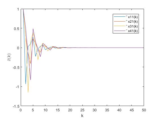
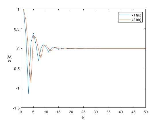
	$\displaystyle\lambda_{1}(\mathcal{A})$	$\displaystyle=$	$\displaystyle 0.1949,\quad\lambda_{2}(\mathcal{A})=0.6791,$
	$\displaystyle\lambda_{3}(\mathcal{A})$	$\displaystyle=$	$\displaystyle\lambda_{4}(\mathcal{A})=0.7317,$

which means that $\mathcal{A}$ in (23) is sable. In this way, following from Theorem 1, the state error estimation $\tilde{x}(k)$ in (35) is stable, which is shown in Fig. 1, where data 1 to data 4 represent the four components of vector $\tilde{x}(k)\doteq\left[\begin{array}[]{cccc}\tilde{x}_{11}(k)&\tilde{x}_{21}(k)&\tilde{x}_{31}(k)&\tilde{x}_{41}(k)\\ \end{array}\right]^{\prime}$ . Moreover, under the observer-feedback Stackelberg strategy (19)-(20), the state $x(k)$ in (1) is also stable which can be seen in Fig. 2, where data 1 and data 2 represent the two components of $x(k)\doteq\left[\begin{array}[]{cc}x_{11}(k)&x_{21}(k)\\ \end{array}\right]^{\prime}$ . Finally, by analyzing Fig. 1 and Fig. 2 and selecting $N=30$ in Theorem 4, the asymptotical optimal property of the cost functions (62)-(69) under the observer-feedback Stackelberg strategy (19)-(20) is guaranteed.

Refer to caption — Figure 1: Trajectory of $\tilde{x}(k)$ in (35) under the observer-feedback Stackelberg strategy (19)-(20).

VI Conclusion

In this paper, we have considered the feedback Stackelberg strategy for two-player leader-follower game with private inputs, where the follower only shares its measurement informaiton with the leader, while none of the historical control inputs and measurement information of the leader are shared with the follower due to the hierarchical relationship. The unavaliable access of the historical inputs for both controllers causes the main difficulty. The obstacle is overcome by designing the observers based on the informaiton structure and the observer-feedback Stackelberg strategy. Moreover, we have shown that the cost functions under the proposed observer-feedback Stackelberg strategy are asymptotical optimal to the cost functions under the optimal feedback Stackelberg strategy.

References

[1] D. Anderson and B. Moore, “Linear optimal control”, Prentice-Hall, Englewood Cliffs, NJ, 1971.
[2] M. Rami, X. Chen, J. Moore and X. Zhou. “Solvability and asymptotic behavior of generalized Riccati equations arising in indefinite stochastic LQ Controls”, IEEE Transactions on Automatic, 46(3): 428-440, 2001.
[3] H. S. Zhang, L. Li, J. J. Xu and M. Y. Fu, “Linear quadratic regulation and stabilization of discrete-time systems with delay and multiplicative noise”, IEEE Transactions on Automatic Control, 60(10): 2599-2613, 2015.
[4] N. W. Bauer, M. Donkers, N. van de Wouw and W. Heemels, “Decentralized observer-based control via networked communication”, Automatica, 49: 2074-2086, 2013.
[5] F. Blaabjerg, R. Teodorescu, M. Liserre and A. V. Timbus, “Overview of control and grid synchronization for distributed power generation systems”, IEEE Transactions on Industrial Electronics, 53: 1398-1409, 2006.
[6] B. Hoogenkamp, S. Farshidi, R. Y. Xin, Z. Shi, P. Chen and Z. M. Zhao, “A decentralized service control framework for decentralized applications in cloud environments”, Service-Oriented and Cloud Computation, 13226: 65-73, 2022.
[7] Q. P. Ha, and H. Trinh, “Observer-based control of multi-agent systems under decentralized information structure”, International Journal of Systems Science, 35(12): 719-728, 2004.
[8] D. Görges, “Distributed adaptive linear quadratic control using distributed reinforcement learning”, IFAC-PapersOnLine, 52(11): 218-223, 2019.
[9] H. Witsenhausen, “A counterexample in stochastic optimum control”, SIAM Journal on Control and Optimization, 6(1): 131-147, 1968.
[10] E. Davison, N. Rau and F. Palmay, “The optimal decentralized control of a power system consisting of a number of interconnected synchronous machines”, International Journal of Control, 18(6): 1313-1328, 1973.
[11] E. Davison, “The robust decentralized control of a general servomechanism problem”, IEEE Transactions on Automatic Control, AC-21: 14-24, 1976.
[12] T. Yoshikawa, “Dynamic programming approach to decentralized stochastic control problem”, IEEE Transactions on Automatic Control, 20(6): 796-797, 1975.
[13] J. Swigart and S. Lall, “An explicit state-space solution for a deffcentralized two-player optimal linear-quadratic regulator”, American Control Conference, 6385-6390, 2010.
[14] X. Liang, J. J Xu, H. X. Wang and H. S. Zhang, “Decentralized output-feedback control with asymmetric one-step delayed information”, IEEE Transactions on Automatic Control, doi: 10.1109/TAC.2023.3250161, 2023.
[15] A. Nayyar, A. Mahajan and T. Teneketzis, “Decentralized stochastic control with partial history sharing: A common information approach”, IEEE Transactions on Automatic Control, 58(7): 1644-1658, 2013.
[16] A. Nayyar, A. Mahajan and T. Teneketzis, “Optimal control strategies in delayed sharing information structures”, IEEE Transactions on Automatic Control, 56(7): 1606-1620, 2011.
[17] X. Liang, Q. Q. Qi, H. S. Zhang and L. H. Xie, “Decentralized control for networked control systems with asymmetric information”, IEEE Transactions on Automatic Control, 67(4): 2067-2083, 2021.
[18] B. C. Wang, X. Yu and H. L. Dong, “Social optima in linear quadratic mean field control withunmodeled dynamics and multiplicative noise” Aisan Journal of Control, 23(3): 1572-1582, 2019.
[19] T. Başar, “Two-criteria LQG decision problems with one-step delay observation sharing pattern”, Information and Control, 38: 21-50, 1978.
[20] P. George, “On the linear-quadratic-gaussian Nash game with one-step delay observation sharing pattern”, IEEE Transactions on Automatic Control, 27: 1065-1071, 1982.
[21] F. Suzumura and K. Mizukami, “Closed-loop strategy for Stackelberg game problem with incomplete information structures” IFAC 12th Triennial World Congress, Australia, 413-418, 1993.
[22] M. B. Klompstra, “Nash equilibria in risk-sensitive dynamic games”, IEEE Transactions on Automatic Control, 45(7): 1397-1401, 2000.
[23] M. Pachter, “LQG dynamic games with a control-sharing information pattern”, Dynamic Games and Applications, 7: 289-322, 2017.
[24] Y. Sun, J. J. Xu and H. S. Zhang, “Feedback Nash equilibrium with packet dropouts in networked control systems”, IEEE Transactions on Circuits and Systems II: Express Briefs, 70(3): 1024-1028, 2022.
[25] Z. P. Li, M. Y. Fu, H. S. Zhang and Z. Z. Wu, “Mean field stochastic linear quadratic games for continuum-parameterized multi-agent systems”, Journal of the Franklin Institute, 355: 5240-5255, 2018.
[26] H. Mukaidani, H. Xu and V. Dragan, “Static output-feedback incentive Stackelberg game for discrete-time markov jump linear stochastic systems with external disturbance”, IEEE Control Systems Letters, 2(4): 701-706, 2016.
[27] S. R. Chowdhury, X. Y. Zhou and N. Shroff, “Adaptive control of differentially private linear quadratic systems”, IEEE International Symposium on Information Theory, 485-490, 2021.
[28] J. J. Xu and H. S. Zhang, “Decentralized control of linear systems with private input and measurement information”, arXiv:2305.14921, 1-6, 2023.
[29] D. Castanon and M. Athans, “On stochastic dynamic Stackelberg strategies”, Automatica, 12: 177-183, 1976.
[30] A. Bensoussan, S. Chen and S. P. Sethi, “The maximum principle for global solutions of stochastic Stackelberg differential games”, SIAM Journal of Control and Optimization, 53(4): 1965-1981, 2015.