Privacy-Preserving Collaborative Split Learning Framework for Smart Grid Load Forecasting
Abstract
Accurate load forecasting is crucial for energy management, infrastructure planning, and demand-supply balancing. The availability of smart meter data has led to the demand for sensor-based load forecasting. Conventional ML allows training a single global model using data from multiple smart meters requiring data transfer to a central server, raising concerns for network requirements, privacy, and security. We propose a split learning-based framework for load forecasting to alleviate this issue. We split a deep neural network model into two parts, one for each Grid Station (GS) responsible for an entire neighbourhood’s smart meters and the other for the Service Provider (SP). Instead of sharing their data, client smart meters use their respective GSs’ model split for forward pass and only share their activations with the GS. Under this framework, each GS is responsible for training a personalized model split for their respective neighbourhoods, whereas the SP can train a single global or personalized model for each GS. Experiments show that the proposed models match or exceed a centrally trained model’s performance and generalize well. Privacy is analyzed by assessing information leakage between data and shared activations of the GS model split.
Index Terms:
Split learning, load forecasting, transformers, decentralized learning, privacy preserving, mutual information.I Introduction
Electricity load forecasting is crucial for energy management systems as it enables planning for power infrastructure upgrades, demand and supply balancing, and power generation scheduling in response to renewable energy fluctuations. Accurate load forecasting can also result in significant cost savings. In 2016, Xcel Energy saved $2.5 million by reducing their load forecasting error from 15.7% to 12.2% [1].
Sensor-based approaches for electricity load forecasting use historical load traces from smart meters and meteorological data to train machine learning (ML) models. ML models for load forecasting can be trained through localized or centralized methods. Localized training entails developing a dedicated model for each smart meter, facilitating client-level load forecasting. Conversely, centralized training involves building a single model using aggregated data from multiple clients to forecast the load for an entire area [2]. However, transferring data directly from clients’ premises to a centralized server imposes a heavy communication load and raises significant privacy and security concerns [3]. For instance, high-resolution smart meter data might disclose when someone is at home, their daily routines, and even specific activities. Moreover, their load signatures can identify certain electrical devices or appliances. For example, the use of medical equipment, home security systems, or specialized machinery can be inferred from the load data [4]. Safeguarding this information is of utmost importance, as it protects an individual’s privacy and ensures compliance with stringent data regulations, such as the European Union General Data Protection Regulation (GDPR) [5]. In addition, the growing adoption of smart meters renders the practice of training individual models for each customer, whether locally or centrally, increasingly impractical from both computational and financial standpoints.
In order to alleviate these problems, decentralized deep learning methods like federated learning (FL) [6] and split learning (SL/SplitNN) [7] have been proposed. These methods decouple the requirement of training an ML model on locally/centrally available data by enabling a group of data holders to train an ML model collaboratively without sharing their private data. In FL, a server contains a global ML model shared among multiple clients. During training, each client receives a copy of the global ML model, generates a model update by improving its private data and sends the updated model back to the server. The server then performs aggregation and updates the global model in some way, usually via weighted averaging, and sends the updated model back to each client. In SplitNN, the ML model is split into two parts, one remains on the client’s side and the other on the server’s side. The client performs the forward pass on its side and shares the outputs with the server, which continues the forward propagation and computes the loss. The gradients are sent back to the client to complete an update step. Clients can choose any ML architecture, as the server has no control over it. In both FL and SplitNN, clients do not share their private data with anyone. These decentralized learning approaches have resulted in a major paradigm shift from an expensive central ML system to utilizing various distributed computational resources.
I-A Related works
This section reviews the recent ML methods proposed for load forecasting, followed by studies that use FL and SL for distributive load forecasting.
I-A1 Load Forecasting
Although the load forecasting problem is not new and several methods have been developed for it [8], we focus on recently proposed deep learning (DL) techniques which have been dominant in sensor-based forecasting [2]. Among these DL architectures, recurrent neural networks (RNN) are well suited for learning the temporal patterns present in smart meter data and have been shown to outperform classical statistical and other ML approaches [2].
Authors in [8] have used the attention mechanism to develop a Sequence to Sequence RNN (S2S RNN) for load forecasting using two RNNs. Their use of an attention mechanism aids in capturing the long-term dependencies present in the load traces by improving the link between both RNNs. In [9], authors used S2S RNN to perform load forecasting for several clients via Similarity Based Chained Transfer Learning (SBCTL), where they train a model for a single client traditionally while the other clients utilize transfer learning to build upon the already trained model. In [10], authors present an online adaptive RNN model to train the model as new data arrives continuously. They use a Bayesian Normalized LSTM (BNLSTM) as their base learner and use an online Bayesian optimizer to update model weights online. Similarly, the authors in [11] propose a multi-layer perceptron mixer structure to perform 24-hour-ahead forecasting.

Following an excellent performance in computer vision (CV) [13] and natural language processing (NLP) community [12], the Transformer architecture [12] (shown in Fig. 1) has recently been employed to capture long-term dependencies in time-series forecasting problems [14, 15, 16]. Instead of working with a single time point at a time (as in RNN), transformer models perform sequence-to-sequence (instead of one sample ahead) forecasting using an encoder-decoder architecture. At the core of transformers, there are self-attention and cross-attention mechanisms which, in vanilla transformer [12], use a point-wise connected matrix leading to a quadratic computational complexity w.r.t. the input sequence size.
For the time-series forecasting problem, the quadratic complexity of the vanilla transformer is prohibitive. Thus, various modifications to the attention mechanism have been proposed to reduce its complexity. Authors in [17] employ log-sparse attention to bring the complexity down to . In [15], Informer architecture is proposed, which uses KL-divergence based ProbSparse self-attention mechanism and a distilling operation to reduce the complexity to . Authors in [14] propose Autoformer, which replaces the canonical attention with an auto-correlation block to achieve sub-series level attention with complexity. In FEDformer [16], similar to [14], authors replace the canonical attention with an attention mechanism implemented in the frequency domain (using FFT or wavelet transform). They perform low-rank approximation in the frequency domain and use the mixture of experts’ decomposition to separate short-term and long-term patterns, leading to linear complexity . Drawing on the comprehensive performance evaluations reported in FEDformer [16] and Autoformer [14], these methods outperform recently proposed transformer-based, LSTM-based, and statistical-based approaches in both univariate and multivariate prediction tasks across a prediction horizon of 4-30 days.
| Scheme | Training Framework Used | Deep Learning Architecture Used | Forecast Horizon (hours) | Models Trained | Privacy Preservation Methodology & Analysis | ||
| Method Applied | Quantitative† | Qualitative‡ | |||||
| Tian et al. [9] | SBCTL | S2S RNN | 1 | Global | |||
| Sehova et al. [8] | Central | S2S RNN | 1, 24 | Global | |||
| Fekri et al. [10] | Central | BNLSTM | 1 - 200 | Global | |||
| Yazici et al. [18] | Central | 1D-CNN, LSTM, GRU | 1, 24 | Global | |||
| Ryu et al. [11] | Central | MLP-Mixer | 24 | Global | |||
| Taik et al. [19] | FL | LSTM | 1 | Global | FL | ✗ | ✗ |
| Li et al. [20] | FL | LSTM | 1 | Global | FL | ✗ | ✗ |
| Liu et al. [21] | FL | LSTM | 1, 7 | Global | FL + HE | - | - |
| Fekri et al. [22] | FL | LSTM | 1, 24 | Global | FL | ✗ | ✗ |
| Yang et al. [23] | FL | SecureBoost | 1 | Global | FL | ✗ | ✗ |
| Liu et al. [24] | FL | RNN + LSTM + GRU | 0.5 - 4 | Global | FL | ✗ | ✗ |
| Husnoo et al. [25] | FL | RNN + LSTM + GRU + CNN | 1 | Global | FL + DP | ✗ | ✓ |
| Liu et al. [26] | FL | Prob-GBRT | 1 | Global & Local | FL | ✗ | ✗ |
| Sakuma et al. [27] | SL | S2S LSTM + GRU + 1D-CNN | 1, 24 | Global & Local | SL | ✗ | ✗ |
| Proposed | SL | S2S FEDformer | 96 | Neighbourhood | SL + DP | ✓ | ✓ |
| Training framework abbreviations: SBCTL: Similarity based Chained Transfer Learning, FL: Federated Learning, SL: Split Learning. | |||||||
| Deep learning model abbreviations: S2S: Sequence to Sequence, RNN: Recurrent Neural Network, LSTM: Long Short-Term Memory, | |||||||
| GRU: Gated Recurrent Unit, BNLSTM: Bayesian Normalized LSTM, CNN: Convolutional Neural Network, | |||||||
| MLP: Multi Layer Perceptron, Prob-GBRT: Probabilistic Gradient-Boosted Regression Trees. | |||||||
| HE: Homomorphic Encryption, DP: Differential Privacy. | |||||||
| : Privacy was not considered while the central model was trained. ✓: Included. ✗: Not included. - : Not applicable. | |||||||
| Quantitiative: Similarity analysis between clients’ data and shared information. | |||||||
| Qualitative: Effects of privacy preservation approach on model performance. | |||||||
I-A2 Decentralized Learning Methods
In their primary forms, both FL and SL frameworks assume that a single model can capture trends across diverse clients; thus, for the load forecasting application, these naive approaches try to learn a single model capable of generating load traces for each client. This, however, is not optimal as the pattern diversity between the clients is usually large, and learning a single forecast model may lead to inferior performance. When used for load forecasting using smart meter data, the methods reviewed so far learn one individual model for each smart meter client or one for a particular group. However, this training strategy becomes computationally expensive as the number of clients grows and raises privacy and security vulnerabilities associated with centralized data transfer.
Several FL and SL-based methods have been proposed to address these issues. In [19], an FL-based method has been presented for short-term (One-hour) load forecasting for smart meters with similar load profiles. Their approach uses LSTM as the learning model and federated averaging architecture with weighted averaging for model weights aggregation. The method is shown to work well for short-term (one hour ahead) predictions. Similarly, [9] presents a similar approach for short-term forecasting with an emphasis on providing security to the framework via encryption schemes. This, however, leads to increased time complexity of the model. In contrast to [19], authors in [22] compare the performance of two FL techniques, FedSGD (single gradient descent step per client) and FedAVG (multiple gradient updates before merging), and allow their clients to have profiles from different distributions. Similarly, recent studies like [24] and [25] have leveraged RNN, LSTM, and GRU architectures to train global models for short-term forecasting within the FL framework. Furthermore, in the work by [25], differential privacy techniques were applied to obscure signs of shared client gradients, providing an additional layer of protection for client privacy. In a recent work [26], the authors introduce an FL-based boosted multi-task learning framework tailored for inter-district collaborative load forecasting (1 hour ahead). The approach revolves around initially training a central model, which is subsequently employed by individual districts to train personalized models capable of capturing their respective local temporal dynamics. A notable feature of this framework is its use of the probabilistic Gradient-Boosted Regression Tree (GBRT) as the base learner.
In [28], authors use the SL framework to split a 1D CNN network model into two halves and use it to detect heart abnormalities from the medical ECG dataset. Furthermore, they show that in the case of 1D CNN, SL may fail to protect the patients’ private raw data. To mitigate this data leakage, they use differential privacy (DP) [29], where carefully computed noise is added to the patients’ activations as an additional layer of security. Their results show that DP does reduce privacy leakage but at the expense of model performance. Similar to [28], another recent SL-based method [30] splits an LSTM network to train a classifier for time-series data of multiple patients. To reduce privacy leakage, differential privacy has been used to break the 1-1 relationship between input and its split activations.
A short summary of related work on the smart grid load forecasting problem is given in Table I.
I-B Problem Description and Motivation
Consider a scenario where an energy provider company distributes power to multiple neighbourhoods/districts of a city. Each community is served by a single Grid Station (GS). The Service Provider (SP) is interested in training a load forecasting model for medium (few hours) to long-term (few days - weeks) forecasting to better manage their generation capacity and reduce energy waste. To do so, they can employ different strategies, e.g., the SP might want to learn a single prediction model for all districts, which is easier but not optimal as households across neighbourhoods may have different load profile distributions. Thus, training a single model to cover all distributions may lead to significant prediction errors. Conversely, training a single model for every client is cumbersome and infeasible if the number of clients is substantial. Instead of either of these extremes, we propose to learn a single model for each neighbourhood as one would expect clients from the same neighbourhood to have similar load profiles, facilitating the training of an accurate prediction model.
Next, we need to decide on a training framework, i.e., central or decentralized. As data privacy is our top priority, decentralized learning strategies like FL and SL should be employed where the private data never leaves the client’s premises. However, as the client-side training has to be performed by a smart meter, the training process’s computational and data transfer requirements have to be modest so as not to hinder their main functionalities. The SL framework is selected to ensure this due to its low computational and communications requirements and privacy-preserving nature.
I-C Contributions
The major contributions of this paper are as follows:
-
•
We propose a novel SL framework with a dual split strategy, i.e., the network’s first split (Split-1) resides at the GS covering a single neighbourhood, and the second split (Split-2) stays at the SPs’ end. To reduce computational load on smart meters, each client is only responsible for performing a forward pass on its private data using their GSs’ Split-1 network, computing the loss, and initiating back-propagation. GS is responsible for carrying out back-propagation through the Split-1 model and updating its weights. The models, as a whole, are trained using two alternative strategies: SplitGlobal, which trains unique Split-1 models for each neighbourhood and a global Split-2 model shared by all neighbourhoods, and SplitPersonal, which trains personalized split models (Split-1 and Split-2) for each neighbourhood. Once the training is complete, the SP will have access to both network splits and can perform individual-level (requiring respective clients’ involvement) and neighbourhood-level predictions using the cumulative load trend from the respective neighbourhood GS.
-
•
As our base learner, we utilize the transformer [12] based architecture, called FEDformer [16]. Compared with widely used LSTM, transformers enjoy better performance and can fully utilize the acceleration offered by discrete graphics processing units. Based on our literature review, ours is the first work that uses a transformer architecture to implement split learning for electricity load forecasting. Extensive experiments are conducted to assess the performance of the trained split model against a centrally trained model under multiple scenarios.
-
•
We present a detailed quantitative assessment of the extent of information leakage between clients’ private data and their respective Split-1 activations using mutual information-based neural estimation (MINE) [31]. Based on the estimated mutual information (MI) between input and activations, a vigilant client can decide whether the current activations batch is secure enough to be forwarded to the GS or not. For additional privacy, we incorporate differential privacy [29, 32] to further obfuscate the client’s Split-1 activations into the model framework and analyze its effects on information leakage and model performance.
The rest of the paper is organized as follows: Section II briefly describes FEDformer, the transformer variant used in this work. We further discuss the concepts of split learning, differential privacy, and mutual information neural estimation. Section III outlines the proposed system model, the FEDformer model split and the SL training framework. Section IV presents experimental evaluations of the proposed framework under different testing scenarios, followed by privacy leakage analysis using mutual information and differential privacy. We conclude the paper in Section V.
II Preliminaries
In this section, we briefly describe the frequency enhanced attention blocks proposed in FEDformer [16], split learning framework [7], differential privacy for machine learning [29], and mutual information neural estimation [31] for privacy leakage analysis.
II-A FEDformer
FEDformer follows the deep decomposition architecture proposed in Autoformer [14], where the input time series is analyzed by decomposing it into a seasonal and a trend-cyclical part. The seasonal part is expected to capture seasonality, whereas the trend-cyclical part is expected to capture the long-term temporal progression of the input. FEDformer uses a series decomposition block with a single or a set of moving average filters (of different sizes) to perform such decomposition. FEDformer implements self-attention mechanisms in the frequency domain using two distinct blocks, a Frequency Enhanced Block (FEB) and a Frequency Enhanced Attention (FEA) Block. Their working is briefly discussed next.
II-A1 Frequency Enhanced Block
In [16], the authors proposed Fourier transform and Wavelet transform to work in the frequency domain. Here we will only focus on the Fourier transform. Let be the input to the FEB, where is the sample length, and is the inner dimension of the model. Query matrix Q is computed by linearly projecting X with as . Next, Q is transformed from time to frequency domain using Discrete Fourier transform (DFT) to get . A subset of randomly selected Fourier components is discarded from to get a reduced dimensional matrix , where . Finally, the output of FEB is computed as
| (1) |
where is a randomly initialized parametric kernel, and is the production operator. The result of is then zero-padded to and transformed back into time domain via inverse DFT.
II-A2 Frequency Enhanced Attention Block
The FEA block takes two inputs, the encoder output and from decoder, and generates the query Q matrix via linearly projecting using weight matrix , whereas the key K, and value V matrices are generated by projecting using and , respectively.
The query, key, and value matrices are then transformed from time to frequency domain via DFT followed by random mode selection (as in FEB Section II-A1) to get . Finally, the output of FEA is computed as
| (2) |
where is the tanh activation function.
II-B Split Learning
In split learning (SL) [7], a deep neural network (DNN) is split into two halves; clients maintain the first half and the remaining layers are maintained by a server. Consequently, a group of clients are able to train a DNN collaboratively using (but not sharing) their collective data. Additionally, the server performs most of the computational work, reducing the clients’ computational requirements. However, this comes at the cost of privacy trade-off, i.e., the output of earlier layers leaks more information about the inputs [33]. Here, choosing a suitable split size is important for expecting data privacy as it has been shown that for a relatively small client model, an honest-but-curious [34] server can extract the clients’ private data accurately just by knowing the client-side model architecture [28]. Thus, it is recommended that in SL, clients should compute more layers, increasing computational load but incurring stronger privacy [28].
During training, clients perform forward passes using their own data up to the final split layer of DNN. These activations are then shared with the server, which continues the forward pass on its DNN split. If the label sharing between clients and servers is enabled, the server can compute the loss itself. Otherwise, it has to send the activations of its final layer back to the client for loss computation. In this case, the gradient backpropagation begins on the client side, and the client feeds the gradient back to the server, which continues backpropagation through its DNN split. Finally, the server shares the gradients at its first layer with the client, who finishes the backpropagation through its DNN split. When more than one client is participating in training, SL adds all clients into a circular queue, whereby each client takes turns using their private data to train with the server. At the end of a training round, the client shares its updated model weights with other clients either through a central server, directly with each other, or via a P2P network.
II-C Differential Privacy
One of the most widely used privacy-preserving technologies is Differential Privacy (DP) [29]. Its effectiveness in safeguarding user data privacy has been extensively demonstrated by adding carefully computed noise to the data. The machine learning community has widely used DP to ensure data privacy [35, 32]. Let be the input space, the output space, the privacy budget parameter, be a non-negative heuristic parameter, be the number of samples in the dataset, and a randomization mechanism. We say that the mechanism is differentially private (-DP) if, for any neighbouring datasets and (differing by a single element) in , and any output , as long as the following probabilities are well-defined, there holds
| (3) |
Intuitively, (3) provides an upper bound () on the difference between outputs of the mechanism when applied to two neighbouring datasets, where the value of controls the overall strength of the privacy mechanism and accounts for the probability that privacy might be violated [32]. Thus, to ensure stronger privacy protection, both and should be kept low. With , the pure DP is shown to be much stronger than the DP (with ) in terms of mutual information [36]. Nevertheless, the DP offers the advantage of advanced composition theorems, enabling a substantially greater number of training iterations compared to pure DP with the same . As a result, most recent works in differentially private machine learning have shifted away from DP.
Let be a deterministic real-valued function. Then, in order to approximate this function with an DP mechanism, noise calibrated with f’s sensitivity () is added to its output. Here, sensitivity is defined as . Intuitively, for high sensitivity, it is much easier for an adversary to extract information about the input [29]. The general mechanism that satisfies the DP is defined by
| (4) |
where is a random variable from distribution under DP or under DP [35]. In our case, is the split model, X is a clients’ private input dataset, sensitivity is computed across the batch axis of the Split-1 activations tensor, and the noise is added to the clients’ batch activations at Split-1 model output. In this way, the noise level is controlled by the sensitivity , which comes from the data, the probability , and the privacy budget , which can be set according to the privacy requirements, e.g., results in a weak privacy guarantee as compared to , which gives the strongest privacy guarantee but makes the data useless. The privacy guarantee of a DP mechanism (4) is that the likelihood of revealing sensitive information about any individual in the input dataset through the algorithm’s output is significantly reduced [35]. In our study, we analyze both DP mechanisms in terms of the mutual information leakage between input and output of the clients’ split network.
II-D Mutual Information Neural Estimation
The clients’ split layer activations in SL frameworks are shared with the server. However, these activations may carry enough information about the input that an adversary might be able to precisely reconstruct the original data [37]. Various researchers have utilized noise addition mechanisms offered by -Differential Privacy as a security measure [28] to mitigate this issue. However, it is difficult to quantify the relationship between the added noise level and the information leakage risk. Mutual information (MI) is commonly used in information theory to assess how much information can be inferred from one random variable (RV) about another. Compared to correlations, MI can capture non-linear statistical dependencies between RVs [31]; however, it is difficult to compute, especially for high-dimensional RVs. In [31], the authors have proposed to compute MI using neural networks using the fact that MI between two IID RVs X and Y is equivalent to the Kullback-Leibler Divergence (KLD) between their joint () and product of their marginal () distributions. According to the Donsker-Varadhan representation of KLD [38], the MI between X and Y is lower bound by
| (5) | |||||
Here is any class of functions that satisfies the integrability constraints of Donsker-Varadhan theorem. Under this setting, the authors in [31] use a neural network to model , which converts the MI problem to a network optimization one, leveraging neural networks’ ability to approximate arbitrary complex functions.
Consider an SL framework where x and y are the batched inputs and outputs of the split network, and we are interested in finding how much information about x can be inferred from y. To do so, we need to estimate the MI between them. Ref. [31] says that this MI is lower bounded by (5). Let be a neural network. Then, the expectations in (5) are empirically estimated by sampling from joint distribution as and from marginals by shuffling y across the batch axis to get . In other words, in the input-output relationship is intact, whereas, in , this relationship has been broken. The network is trained by maximizing (5). Thus, if MI between a batched x and y is large, (5) computed using a trained network will be high, and vice versa. We demonstrate this effect in detail in Section IV-E1.

III Proposed Split Learning Framework for Electricity Load Forecasting
In this section, we first discuss the proposed system model, the adversarial model, the FEDformer model split and their internal modules, followed by our proposed split learning framework and its training methodology.
III-A System Model
We consider a three-tier system model with four major entities, as shown in Fig. 2. On top, we have the electricity Service Provider; in the middle, we have Grid Stations responsible for distributing electricity to the individual districts/neighbourhoods. The lowest tier comprises smart meter clients (industrial, commercial, or residential) lumped into neighbourhoods. Under this model, the SP is an organization which procures electricity from various providers and is responsible for meeting the energy requirements of all connected GSs. Moreover, the smart meters can connect to their GS using a secure communications protocol, e.g., cellular network or power-line communications. The GSs are connected to SP via a private network or the Internet. The SP can not connect directly with any client and has to go through the GS to communicate with a client. The objective is to learn a DL time series prediction model, using a split learning framework, on all clients’ data without compromising the individual clients’ privacy. Once trained, the entire model will be accessible to the SP, and the SP can effectively perform medium to long-term load forecasting for any client from any neighbourhood.
III-B Adversary Model
In this paper, we assume a modest security environment, i.e., the GS, SP, and the clients are honest-but-curious [34, 28]. Thus, the participants may not try to poison the training process; however, both the GS and SP may collude to infer information about clients’ private data as they have access to the entire model and the client-side split layer activations (details in Section III-D). Furthermore, external adversaries or some malicious clients may try to intercept the split layer activations sent by the other clients to GS to extract their private data. Thus, the attack model considered here is the model inversion attack, which aims to extract clients’ sensitive data given only their activations. Under this attack, the objective of the adversary is to find a function which can infer the client’s private data X from its split activations A as . However, in practice, this inference need not be exact, as a close approximation of the client’s data is usually enough.

III-C The FEDformer Model Split
We have selected FEDformer architecture [16] (with some modifications) as our backbone prediction model, where the entire model consists of two encoders and a single decoder block. The FEDformer model is split into two halves, termed Split-1 and Split-2. The Split-1 model contains the first two inner blocks of the FEDformer encoder and FEDformer decoder, whereas the Split-2 model contains the remaining inner blocks of the first FEDformer encoder followed by a complete FEDformer encoder block and remaining inner blocks of the FEDformer decoder. Each GS gets its own copy of the Split-1 model, and the SP maintains Split-2. The resulting split FEDformer is shown in Fig. 3. In Section II-A we have discussed the series decomposition, FEB and FEA blocks, and the rest are briefly discussed next.
The data embedding layer included in model Split-1, as shown in Fig. 3, consists of a series decomposition layer, a 1D convolutional layer, and two linear layers. It takes three inputs, an input time-series of length L , where is the dimension of each time point (for univariate case, ), the timestamp encoded information of the input time-series as , and output time-series , where depends upon the temporal granularity, and denotes the prediction time horizon, for instance, for the scale of Year-Month-Day-Hour, . First, X is passed through the series decomposition block to get a seasonal component and a trend component . Then, the embedded inputs to the encoder and decoder blocks of Split-1 are generated as:
| (6) |
where denote the placeholders filled with zeros and mean of X, respectively, , , and . Here, is the inner dimension of the model. In this way, the decoder takes guidance from the later half of the input time series to fill in the remaining placeholder data points during training. Since the series-wise connection will inherently keep the sequential information, we do not need to perform position embedding, which differs from vanilla Transformers. This specific setting for the Split-1 network was chosen to keep the computational requirements low while ensuring a complex non-linear relationship between the input and outputs of Split-1 to ensure low information leakage between them (see details in Section IV-E1).
The feed-forward network, seen in the Split-2 encoder and decoder, is a two-layer fully connected neural network (FCNN) with input and output dimensions , and inner dimension . The output of its first layer is passed through GELU activation function before passing to layer two. The output (seasonal and trend) tensors generated by series decomposition blocks found in Split-1 and Split-2 decoders have dimensions , whereas the incoming and containing temporal trend information are dimensional (dimension of the input time series). Thus, the trend output tensor of a series decomposition block is first projected back into dimensional tensors using trainable projection matrices , where , before adding to the incoming trend tensors. Similarly, the seasonal tensor of the final series decomposition block of the Split-2 decoder is also projected down to before adding to the incoming trend tensor to generate the final prediction output.
III-D Proposed Split Learning Framework
Figure 2 depicts the SL training process for load forecasting. Note that the clients do not transfer prediction targets (labels) to the GS or SP. As discussed in Section III-C, the FEDformer is split into two halves, and each GS maintains a personalized copy of model Split-1. The model Split-2 resides at the SP. Unlike a traditional Split Learning framework where clients are responsible for the forward pass, backpropagation through their network split, and parameter updates, our framework proposes a different approach. In our proposed framework, smart meters perform only the forward pass through their data, compute loss (after receiving predictions from SP through GS), and initiate backpropagation (gradient computation of loss with respect to the predictions only). The GS performs backpropagation through Split-1 and parameter updates, significantly reducing the computational load on the smart meters. As a byproduct, we do not need to over-simplify the Split-1 model; thus, non-linear relationships between clients’ inputs and activations are maintained, ensuring stronger privacy.
Two strategies are employed when training at SP, i.e., SP can learn a single Split-2 model for all GSs (neighbourhoods) or one personalized Split-2 model per GS. In the case of the former, the overall learned model is referred to as SplitGlobal, whereas the latter model is called SplitPersonal. The goal is to analyze the generalization capabilities of the model when performing predictions for clients from the same as well as those coming from different neighbourhoods, as clients from different neighbourhoods are expected to have different load patterns and distributions. Nevertheless, the training process is relatively similar for both models. Algorithm 1 outlines the pseudo-code for training the SplitGlobal variant of the proposed SL model.
We start with weight initialization for all SP and GS models. At the start of each training epoch, A GS selects all or a subset of neighbourhood clients (chosen randomly or the same as the previous epoch).
Following this, the training begins in parallel across all GSs, where the participating clients use a single private training batch to perform the model update in 7 distinct sequential steps (see Fig. 2). These steps are summarized in relation to Algorithm 1 next.
Steps 1-2: Each GS sends its Split-1 model weights to all selected neighbourhood clients . In parallel, each receiving client performs a forward pass through the received Split-1 model using one of its private training batches . The activations of the final split layer, denoted by of Split-1 model are forwarded to the GS (lines 8-11 of Algorithm 1).
Step 3: Once a GS has received batched activations from all of its training clients, it concatenates their activations, denoted by , and forwards them to the SP to continue the forward pass (lines 12-13 of Algorithm 1).
Step 4: Depending upon the model being trained, i.e., SplitGlobal or SplitPersonal, this step is performed little differently. In the case of SplitGlobal, the SP performs the forward pass through a single Split-2 model using a batch size of , where denotes the number of clients (lines 14-15 of Algorithm 1). For SplitPersonal, the SP performs a forward pass through the individual personalized Split-2 models using the activations received from their respective GSs.
Step 5: As the training data is never allowed to leave the client’s premises, the final Split-2 layer outputs are forwarded to their respective clients through GSs for loss computation (lines 17-19 of Algorithm 1).
Step 6: Each client computes loss, initiates back-propagation and shares gradients w.r.t. outputs with their GS, that forwards these gradients to SP (lines 20-22 of Algorithm 1).
Step 7: Once gradients from all GSs are received,
SP continues the gradient back-propagation through its Split-2 model(s). The gradients w.r.t. each are then forwarded back to their respective GSs. Each GS averages the received gradients across clients’ dimensions and continues back-propagating through their respective Split-1 models (lines 24-25 of Algorithm 1).
Step 8: Once all gradients have been populated, SP and each GS update their model weights (line 26 of Algorithm 1).
Following the model updates, the GSs pass their updated models back to their respective clients for another round of batch training. This is repeated until all batches have been iterated over, thus completing a single training epoch. For the next epoch, GSs can continue training with the same clients or select new ones. Once training is finished, each GS will have a personalized Split-1 model.
IV Experimental Evaluation
In this section, we provide a detailed experimental evaluation of the proposed framework under multiple testing scenarios and present the mutual information-based privacy leakage analysis resulting from sharing activations with and without differential privacy.
IV-1 Dataset and Evaluation Metrics
We used the Electricity111https://tinyurl.com/fxbcbufp dataset [14]222https://github.com/thuml/Autoformer for performance evaluation, which includes hourly electricity consumption of 320 smart meters from July 2016 - July 2019. We selected the first 17,566 entries from July 2016 to July 2018 for training to minimize training time. After normalizing each client’s time series to zero mean and unit variance, we used the agglomerative clustering algorithm to group them into three clusters, consisting of 54, 201, and 65 clients, respectively. For visualization, five randomly selected examples from each cluster over 9 days of data are shown in Fig. 4. Cluster 1 had the most diverse electricity usage patterns, with load patterns and magnitudes varying significantly across clients in each cluster.
The objective of the proposed framework is thus to learn DL models which can accurately perform predictions for clients from each of the three neighbourhoods. We divide each client’s load time series into train-val-test sets for training and evaluation purposes according to a 7:1:2 ratio. The evaluation metrics selected are the mean absolute error (MAE), mean square error (MSE), and the coefficient of determination () between the true and predicted trajectories. The metric highlights the goodness of fit of a prediction model and is computed as:
| (7) |
where is the true time series and is the model prediction.

IV-2 Implementation Detail
All of our experiments were performed on Python 3.8, and model implementations were forked from FEDformers’ GitHub implementation333https://github.com/MAZiqing/FEDformer. We keep the default parameters from FEDformer unchanged unless specified otherwise. Models were trained using ADAM optimizer with adaptive learning rates starting at and a batch size of 32, with MSE as our training loss. Training is performed over 10 epochs, and an early stopping counter of 3 epochs is used to stop the training once the error over the validation set stops to improve. The input sequence length is set at hours, output/prediction horizon is set to hours, model inner dimension , and randomly selected modes are used in FED and FEA blocks. Both FED and FEA are implemented with attention heads. We choose clients per neighbourhood in 3 neighbourhoods, with one GS assigned to each neighbourhood. Experiments are repeated 3 times and average results are reported. The split FEDformer contains 2 encoder and 1 decoder layers (see Fig. 3).
All DL models are implemented in PyTorch v1.9 [39] and training is performed on a single Nvidia Tesla V100-32 GB GPU available through a volta-GPU cluster of the NUS-HPC system444https://nusit.nus.edu.sg/hpc/. To implement differential privacy, we used the open-source Diffprivlib library [40]. The implementation code is publicly available at [41].
| MAE | MSE | ||||||||
|---|---|---|---|---|---|---|---|---|---|
| SL-G | SL-P | Central | SL-G | SL-P | Central | SL-G | SL-P | Central | |
| GS 1 | 0.451 | 0.453 | 0.513 | 0.387 | 0.383 | 0.540 | 0.396 | 0.405 | 0.346 |
| GS 2 | 0.256 | 0.253 | 0.246 | 0.133 | 0.130 | 0.133 | 0.863 | 0.868 | 0.855 |
| GS 3 | 0.372 | 0.361 | 0.355 | 0.256 | 0.241 | 0.252 | 0.663 | 0.687 | 0.671 |
| Mean | 0.360 | 0.356 | 0.371 | 0.259 | 0.251 | 0.308 | 0.641 | 0.653 | 0.624 |
IV-A Comparison with Centralized Model
In our first experiment, we compare the performance of models trained under the proposed SL framework with a centrally trained FEDformer model. To do so, we train SplitGlobal and SplitPersonal models for 3 GSs and 10 clients per GS. The clients are kept fixed during all training epochs. For the centralized model, we choose the same 10 clients from each GS (30 clients total), as used by our proposed models to train a univariate FEDformer model in a centralized manner. The objective is not only to validate our proposed SL training framework but also to assess the efficacy of training multiple models w.r.t. a single central one. The resulting MAE, MSE, and scores on the test sets of clients belonging to different neighbourhoods are summarized in Table II. The MAE, MSE, and metric scores for GS 2 and 3 for all 3 models are relatively similar, with the Centrally trained model edging the proposed models slightly in terms of MAE, whereas, in terms of MSE and , the SplitPersonal model performing better. These results show that all 3 models could generalize the load patterns for GS 2 and 3’s neighbourhood clients. The load profiles of these clients were not too erratic compared to clients belonging to neighbourhood 1, for whom the centrally trained model performed objectively worse.
As discussed in Section IV-1, the load profiles for clients belonging to cluster 1 (GS 1) show high diversity and are the most challenging out of the three. Observing the superior performance of the proposed models as compared to the central model shows that expecting a single central model to perform well for a diverse range of load profiles is not viable. Moreover, learning multiple models for data from similar distributions should work comparatively well. Thus, the proposed framework essentially offers a balanced approach between learning a single model for all clients and learning a single model for each client.
When comparing scores of SplitGlobal and SplitPersonal, we see that the latter performs well both in terms of individual GS scores and average ones. This, however, is expected as for SplitPersonal, the SP trains personalized Split-2 networks for each GS. Thus it should be able to generalize well for the respective neighbourhoods. To visualize the model convergence, we present the MSE scores for train, validation, and test sets for the 3 models in Fig. 5. Here, we see that although the central model achieved the lowest training error, its validation and test set errors are the highest, owing to over-fitting to the training data. We can say this because most, if not all, of the difference between central and proposed methods test set scores, is coming from its prediction scores for the GS 1s’ load profiles (see MSE scores given in Table II). As otherwise, the test scores for the central model over GS 1 and 2 were very close to the proposed model’s scores. The run-times of a single epoch for SplitGlobal, SplitPersonal, and Central models are 20, 20, and 40 minutes respectively.

IV-B Across neighbourhood predictions
In our next experiment, we analyze the trained models’ prediction ability when the tested data comes from another GSs’ neighbourhood, i.e., from a different distribution. The MSE scores for both models are reported in Table III, where rows GS 1-3 denote the trained split models and columns denote the neighbourhoods. Thus, the table cell for row GS 1 and column 1 represent the MSE score for neighbourhood 1’s test data when GS 1’s model is used for prediction. Consider GS 1 models’ scores for all neighbourhoods (top row) under both SP training strategies. We see that, apart from testing scores for their own neighbourhood data, the SplitGlobal models’ prediction errors for neighbourhoods 2 and 3 are well below those reported by SplitPersonal model (see Fig. 6 for individual scores). This is attributed to the fact that under SplitGlobal, the SP learns a single global Split-2 model, which is jointly trained to learn from all neighbourhood clients. Whereas, under SplitPersonal training strategy, the SP learns 3 personalized Split-2 models, which have never seen the data coming from different neighbourhoods. Similar trends can be observed for models GS 2 and 3 where cross-neighbourhood scores reported by SplitGlobal are better. Similarly, the mean scores for a single neighbourhood overall GS 1-3 models also show that SplitGlobal has better generalization capabilities as compared to SplitPersonal.
SplitGlobal - MSE SplitPersonal - MSE 1 2 3 Mean 1 2 3 Mean GS 1 0.390 0.249 0.353 0.331 0.385 0.379 0.434 0.399 GS 2 0.442 0.134 0.343 0.306 0.522 0.130 0.345 0.332 GS 3 0.434 0.186 0.259 0.293 0.426 0.204 0.240 0.290 Mean 0.422 0.190 0.319 0.445 0.238 0.340
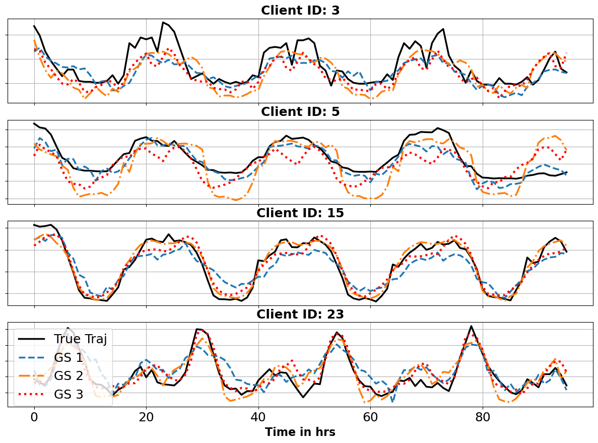
To visualize individual test scores for each neighbourhood client under different learned models, we present their MAE scores in Fig. 6. Here, the first 10 clients are from neighbourhood 1 and so on. For all 3 models, we see that the most MAE variation is found in neighbourhood 1’s clients, whereas for 2nd and 3rd neighbourhoods, the variations are small. Moreover, for each neighbourhood, their respective GS models perform best. We further present example batch predictions for 4 clients in Fig. 7. Looking at predictions from both models, we see that for clients 15 and 23, all three GS models do follow the true trajectory very closely, with SplitGlobal’s cross neighbourhood predictions being slightly better. However, for clients 3 and 5, belonging to neighbourhood 1, discrepancies are large, especially for cross-neighbourhood predictions of client 5. Moreover, SplitPersonal’s GS 1 model followed the true trajectory much more closely, especially near the prediction endpoints.

 |
 |
| SplitGlobal | SplitPersonal |
Same Clients Random Clients Post Add. Tr. SL-G SL-P SL-G SL-P SL-G SL-P GS 1 0.390 0.385 0.650 0.644 0.528 0.511 GS 2 0.134 0.130 0.166 0.161 0.154 0.147 GS 3 0.259 0.240 0.218 0.295 0.214 0.264 Mean 0.261 0.252 0.345 0.367 0.299 0.308
IV-C Predictions on unseen data
In this experiment, we test the trained models’ prediction abilities for clients that are completely new to them. Under usual circumstances, we might not be able to use every client for training; thus, the trained models’ generalization capabilities need to be tested. To do so, we start with the models trained on the same 10 clients per neighbourhood and test them on 10 randomly selected clients from each neighbourhood. The results of this test are given in Table IV, where we see that clients coming from 2nd and 3rd neighbourhoods receive slightly worse prediction errors, whereas for neighbourhood 1, the error increases by almost 66%. This performance loss, again, can be attributed to the data diversity found in clients from Neighbourhood 1. To investigate whether further training using these clients brings improvement, we train the model for 5 additional epochs using the selected random clients, whose testing results are summarized in the last two columns of Table IV. We see that additional training not only reduced the error for neighbourhood 1 from 66% to 35%, but also improved scores for the rest of the neighbourhood clients.
IV-D Training with random clients
In this experiment, we compare the prediction performance of models when trained using the same clients (10 per GS) compared to randomly selected clients at every training epoch. The models were trained for 10 epochs and tested against randomly chosen clients, and their results are shown in Table V. Comparing SplitPersonals’ GS 1 performance for both training schemes; we see that scores for the model trained using random clients are significantly lower than those trained using the same clients. This could be attributed to the fact that in the former case, the model sees several unique clients during the training stage and is thus able to generalize well for unseen data. Apart from this case, the remaining scores are very similar across the two training schemes. From this observation, we can conclude that training using randomly chosen clients every epoch should enable the models to perform well when presented with unseen data. However, as discussed in the previous section, performing a few training iterations using the unseen data should be performed to get improved results.
| Same Clients | Random Clients | |||
|---|---|---|---|---|
| SL-G | SL-P | SL-G | SL-P | |
| GS 1 | 0.650 | 0.644 | 0.638 | 0.551 |
| GS 2 | 0.166 | 0.161 | 0.164 | 0.157 |
| GS 3 | 0.218 | 0.295 | 0.224 | 0.294 |
| Mean | 0.345 | 0.367 | 0.342 | 0.334 |
IV-E Privacy preservation using differential privacy
Under the proposed framework, both network splits are trained outside the clients’ premises, and the training is fully controlled by GS and SP entities. Under the honest but curious security assumption, GS and SP shall not deviate from the training process. However, they may try to infer clients’ private data from the received Split-1 activations. In order to secure clients’ private data, we propose to use -DP [29, 28] to safeguard against such inference attacks. However, before we do this, we first analyze information leakage between the input and output of the proposed Split-1 FEDformer model. To this end, based on the discussion presented in Section II-D, we perform MI estimation using a fully connected neural network (FCNN). A similar strategy has also been used in [42] to infer MI between inputs and gradients of an NN under the FL framework.
IV-E1 Information leakage analysis
We use a 3-layer FCNN as our MI neural estimator (MINE), with layers containing 100, 50, and 1 neuron, respectively. The first and second layers use the exponential linear unit (ELU) as their activation function. The loss function, given in (5), is maximized using ADAM optimizer with a learning rate of . The batch size is kept at , and the model was trained over epochs. Consider an input tensor for Split-1 model (see Fig. 3) of size , where is the batch size, is the input sequence length, and each time points consists of 1 load value and 4-dimensional date-time encoded vector. The output tensor of Split-1 Encoder block is of size , where is the inner model dimension. We aim to find the mutual information leakage between and for a fully trained Split network.
To establish a baseline, we first train the MINE to find the MI between and itself using a randomly selected client from neighbourhood 2. In order to reduce the computational time, MI is estimated for every 10th batch. The mean and spread over one std of MI computed for each batch is shown in Fig. 8 with approximately a final mean MI value . The spread seen above and below the mean line signifies the variations of computed MI values over different example batches. With our experimental setting, we can say that the maximum MI between two variables can be at most on average. Having found the upper limit on MI, we next approximate MI between input and a noise tensor of size equal to to establish a lower limit. The entries of noise tensor were generated from Laplace distribution . The MI score trend for this setting (input - noise only) is also given in Fig. 8 with a final mean value of approx. . Next, we approximate MI between input and clean as well as noise-contaminated and plot them in the same Fig. 8 as well. The final MI for clean and noisy outputs were approx. and , respectively.
Based on the MI approximations discussed above, we see that the MI between input and clean and noisy outputs has a large difference due to the non-linear relationship induced by the Split-1 network. Moreover, the MI of the clean output is much closer to the noise-only case, signifying that the Split-1 network results in minimal information leakage, making the inference attacks much harder to execute [42]. Additionally, as the MI can be computed at the client’s end, the client can make an informed decision as to whether current batched activations are safe enough for sharing with the GS.

IV-E2 Analysis under DP
In this section, we analyze the performance impact of DP (pure DP) on model training and testing. To do so, we select a single client from neighbourhood 2 and train the split model under SplitPersonal setting. However, this time, the client uses the Laplace mechanism [35, 40] to apply DP to its layer activations (both and , see Fig. 3) before forwarding to the GS. The level of noise added is controlled by the privacy budget parameter , where the noise level is inversely proportional to . Thus, a lower results in strong privacy guarantees as compared to higher ones.

To analyze the effects of various privacy budgets, we trained the model with and computed the test scores for the models’ predictions. At the training epoch, we also trained our MINE for every 10th batch to approximate the MI between input and Split-1 layer activations. The MI trends for multiple are shown in Fig. 9, and their respective final MI values, as well as error metrics, are presented in Fig. 10. From Fig. 9 we see that the model trained with has the lowest approximated MI at , which is very close to the MI between input and noise only case seen in Fig. 8. As a result of large noise additions, its respective MAE and MSE scores are the worst. However, in terms of MAE, they are only 36% higher than MAE of the non-DP case. Furthermore, increasing leads to an increase in MI. However, for , the MI stagnates and stays very close to , which is the MI of the non-DP case. In this range, the error metrics are within a margin of error to the non-DP case. This shows that the model can handle DP noise for a low of 5.0. Even for an (medium privacy), the MAE and MSE are only 16% and 26% above the non-DP case, showing that good privacy protection can be achieved with mild performance reduction.

IV-E3 Analysis under DP
Compared to the stricter pure DP [36], -DP introduces an extra parameter, , to the framework. The rationale behind this enhancement is to provide a level of plausible deniability, allowing for a small probability () that an individual’s data might be exposed or identified. While governs the average privacy loss incurred, plays a role in controlling the worst-case privacy loss scenario. Another advantage of differential privacy is its advanced composition theorems, which enable significantly more training iterations than pure DP under the same . This is the reason why most related works in differentially private machine learning have shifted away from pure differential privacy.
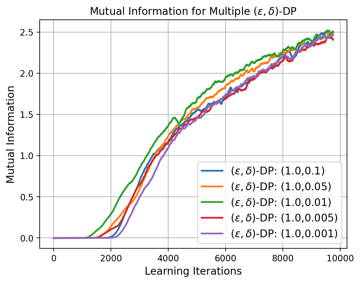
To investigate the impact of -DP on MI leakage and model performance, we repeat the previous experiment but with the -DP via Gaussian mechanism [40]. In this experiment, we maintained at a fixed value of and systematically varied within the range , representing a transition from higher worst-case privacy loss to lower levels. The resultant MI leakage, estimated by our estimator (MINE), between clients’ input data and Split-1 layer activations is presented in Figure 11. Interestingly, the variations in had negligible effects on average privacy loss, as primarily governs the worst-case scenario. Furthermore, Figure 12 displays the model’s prediction accuracy over the entire range of values. These metrics indicate that neither MAE nor MSE exhibit substantial variations within the considered range of values. The performance remains consistent and closely mirrors the outcomes observed when , as depicted in Figure 10.

IV-F Discussion
In Section IV, we used two SL strategies, SplitPersonal where we train neighbourhood-level personalized split networks, and SplitGlobal where a single global Split-2 is trained at SP for all personalized Split-1 models at GSs. Networks trained under both strategies achieved better or comparable performance compared to a centrally trained network, as seen in Table II. When predicting across neighbourhood clients, SplitGlobal model was able to get lower errors as compared to SplitPersonal, as shown in Table III, which is expected.
In Section IV-C, we tested the trained models on data from clients not used during the training stage. The results in Table IV show that the trained models performed well in this scenario; however, additional training using the new client’s data improved performance. This is essential as new clients are constantly added to the system, and we might have very little data on them. Additionally, in Section IV-D, we compare the performance of models trained on the same clients vs training on random clients every epoch against unseen data and found that the models trained on random clients performed better. As with the availability of large amounts of smart meter data, training using all of it is often not feasible. Instead, training using a random subset of clients every epoch can lead to a model with good generalization capabilities. Furthermore, this model can be refined using unseen clients’ data for added performance.
In Section IV-E, we analyzed the extent of privacy leakage arising from the sharing of clients’ activations using MINE. In Fig. 8, we showed that even without the added noise, the Split-1 activations have significantly low MI w.r.t. the inputs due to their non-linear and complex relationship induced by the Split-1 model. Moreover, based on the estimated MI, a client can decide whether to forward the current batch activations to GS or not to mitigate privacy leakage. We further analyze the effects of introducing differential privacy as an additional layer of security on the model’s performance. In Fig. 10, we see that with a moderate privacy budget of , the models performed similarly to the non-DP case and saw performance degradation only when , leading to strong privacy. With a trained model, the electricity service provider can perform individual-level predictions (requiring respective clients’ involvement) and neighbourhood-level predictions using the cumulative load trend from the grid station servicing the neighbourhood. The LSTM-based FL models [22, 19] proposed so far were able to make 1h to 24h ahead predictions; our transformer-based model can perform accurate predictions from 24h - 720h [16], although our experiments were limited to 96h ahead predictions only.
V Conclusion
In this article, we propose a split learning framework to train a DL time series prediction model using the client smart meter data without compromising individual clients’ privacy. Our proposed SL frameworks use the smart meters to perform a forward pass through the Split-1 network only, while the rest of the training is relegated to GS and SP entities. This ensures that the main functionalities of the smart meter remain unhindered. Once trained, the entire model is retained by the energy provider and can be used to perform load predictions for a single smart meter or the entire neighbourhood. The experimental results have shown the performance of the trained models to be better or on par with a centrally trained model. To analyze the extent of information leakage through the Split-1 network, we used mutual information neural estimation to approximate the MI between the input and output of the Split-1 network. The analysis showed that the MI leakage through the Split-1 network is limited. Furthermore, as an added layer of security, we analyzed the addition of -DP and -DP to our framework under multiple privacy budgets. We found that the models performed similarly to the non-DP case under a medium privacy budget while observing low-performance degradation under relatively low privacy budgets.
References
- [1] G. Notton and C. Voyant, “Forecasting of intermittent solar energy resource,” in Advances in Renewable Energies and Power Technologies. Elsevier, 2018, pp. 77–114.
- [2] A. Arif, N. Javaid, M. Anwar, A. Naeem, H. Gul, and S. Fareed, “Electricity load and price forecasting using machine learning algorithms in smart grid: A survey,” in Workshops of the International Conference on Advanced Information Networking and Applications. Springer, 2020, pp. 471–483.
- [3] N. Truonga, K. Suna, S. Wanga, F. Guittona, and Y. Guoa, “Privacy preservation in federated learning: Insights from the gdpr perspective,” 2020. [Online]. Available: https://arxiv.org/abs/2011.05411
- [4] A. Reinhardt, D. Burkhardt, M. Zaheer, and R. Steinmetz, “Electric appliance classification based on distributed high resolution current sensing,” in 37th Annual IEEE Conference on Local Computer Networks-Workshops. IEEE, 2012, pp. 999–1005.
- [5] C. J. Hoofnagle, B. Van Der Sloot, and F. Z. Borgesius, “The european union general data protection regulation: what it is and what it means,” Information & Communications Technology Law, vol. 28, no. 1, pp. 65–98, 2019.
- [6] K. Bonawitz, H. Eichner, W. Grieskamp, D. Huba, A. Ingerman, V. Ivanov, C. Kiddon, J. Konečnỳ, S. Mazzocchi, B. McMahan et al., “Towards federated learning at scale: System design,” Proceedings of Machine Learning and Systems, vol. 1, pp. 374–388, 2019.
- [7] P. Vepakomma, O. Gupta, T. Swedish, and R. Raskar, “Split learning for health: Distributed deep learning without sharing raw patient data,” arXiv preprint arXiv:1812.00564, 2018.
- [8] L. Sehovac and K. Grolinger, “Deep learning for load forecasting: Sequence to sequence recurrent neural networks with attention,” IEEE Access, vol. 8, pp. 36 411–36 426, 2020.
- [9] Y. Tian, L. Sehovac, and K. Grolinger, “Similarity-based chained transfer learning for energy forecasting with big data,” IEEE Access, vol. 7, pp. 139 895–139 908, 2019.
- [10] M. N. Fekri, H. Patel, K. Grolinger, and V. Sharma, “Deep learning for load forecasting with smart meter data: Online adaptive recurrent neural network,” Applied Energy, vol. 282, p. 116177, 2021.
- [11] S. Ryu and Y. Yu, “Quantile-mixer: A novel deep learning approach for probabilistic short-term load forecasting,” IEEE Transactions on Smart Grid, pp. 1–1, 2023.
- [12] A. Vaswani, N. Shazeer, N. Parmar, J. Uszkoreit, L. Jones, A. N. Gomez, L. Kaiser, and I. Polosukhin, “Attention is all you need,” Advances in neural information processing systems, vol. 30, 2017.
- [13] Y. Rao, W. Zhao, Z. Zhu, J. Lu, and J. Zhou, “Global filter networks for image classification,” Advances in Neural Information Processing Systems, vol. 34, pp. 980–993, 2021.
- [14] H. Wu, J. Xu, J. Wang, and M. Long, “Autoformer: Decomposition transformers with auto-correlation for long-term series forecasting,” Advances in Neural Information Processing Systems, vol. 34, pp. 22 419–22 430, 2021.
- [15] H. Zhou, S. Zhang, J. Peng, S. Zhang, J. Li, H. Xiong, and W. Zhang, “Informer: Beyond efficient transformer for long sequence time-series forecasting,” in Proceedings of the AAAI Conference on Artificial Intelligence, vol. 35, 2021, Conference Proceedings, pp. 11 106–11 115.
- [16] T. Zhou, Z. Ma, Q. Wen, X. Wang, L. Sun, and R. Jin, “Fedformer: Frequency enhanced decomposed transformer for long-term series forecasting,” in International Conference on Machine Learning. PMLR, Conference Proceedings, pp. 27 268–27 286.
- [17] S. Li, X. Jin, Y. Xuan, X. Zhou, W. Chen, Y.-X. Wang, and X. Yan, “Enhancing the locality and breaking the memory bottleneck of transformer on time series forecasting,” Advances in neural information processing systems, vol. 32, 2019.
- [18] I. Yazici, O. F. Beyca, and D. Delen, “Deep-learning-based short-term electricity load forecasting: A real case application,” Engineering Applications of Artificial Intelligence, vol. 109, p. 104645, 2022. [Online]. Available: https://www.sciencedirect.com/science/article/pii/S0952197621004516
- [19] A. Taïk and S. Cherkaoui, “Electrical load forecasting using edge computing and federated learning,” in ICC 2020-2020 IEEE International Conference on Communications (ICC). IEEE, 2020, Conference Proceedings, pp. 1–6.
- [20] J. Li, Y. Ren, S. Fang, K. Li, and M. Sun, “Federated learning-based ultra-short term load forecasting in power internet of things,” in 2020 IEEE International Conference on Energy Internet (ICEI). IEEE, 2020, Conference Proceedings, pp. 63–68.
- [21] H. Liu, X. Zhang, X. Shen, and H. Sun, “A federated learning framework for smart grids: Securing power traces in collaborative learning,” arXiv preprint arXiv:2103.11870, 2021.
- [22] M. N. Fekri, K. Grolinger, and S. Mir, “Distributed load forecasting using smart meter data: Federated learning with recurrent neural networks,” International Journal of Electrical Power & Energy Systems, vol. 137, p. 107669, 2022.
- [23] Y. Yang, Z. Wang, S. Zhao, and J. Wu, “An integrated federated learning algorithm for short-term load forecasting,” Electric Power Systems Research, vol. 214, p. 108830, 2023.
- [24] Y. Liu, Z. Dong, B. Liu, Y. Xu, and Z. Ding, “Fedforecast: A federated learning framework for short-term probabilistic individual load forecasting in smart grid,” International Journal of Electrical Power & Energy Systems, vol. 152, p. 109172, 2023. [Online]. Available: https://www.sciencedirect.com/science/article/pii/S0142061523002296
- [25] M. A. Husnoo, A. Anwar, N. Hosseinzadeh, S. N. Islam, A. N. Mahmood, and R. Doss, “A secure federated learning framework for residential short term load forecasting,” IEEE Transactions on Smart Grid, pp. 1–1, 2023.
- [26] H. Liu, X. Zhang, H. Sun, and M. Shahidehpour, “Boosted multi-task learning for inter-district collaborative load forecasting,” IEEE Transactions on Smart Grid, pp. 1–1, 2023.
- [27] Y. Sakuma and H. Nishi, “Hierarchical multiobjective distributed deep learning for residential short-term electric load forecasting,” IEEE Access, vol. 10, pp. 69 950–69 962, 2022.
- [28] S. Abuadbba, K. Kim, M. Kim, C. Thapa, S. A. Camtepe, Y. Gao, H. Kim, and S. Nepal, “Can we use split learning on 1d cnn models for privacy preserving training?” in Proceedings of the 15th ACM Asia Conference on Computer and Communications Security, 2020, Conference Proceedings, pp. 305–318.
- [29] C. Dwork and A. Roth, “The algorithmic foundations of differential privacy,” Foundations and Trends® in Theoretical Computer Science, vol. 9, no. 3–4, pp. 211–407, 2014.
- [30] L. Jiang, Y. Wang, W. Zheng, C. Jin, Z. Li, and S. G. Teo, “Lstmsplit: Effective split learning based lstm on sequential time-series data,” arXiv preprint arXiv:2203.04305, 2022.
- [31] M. I. Belghazi, A. Baratin, S. Rajeswar, S. Ozair, Y. Bengio, A. Courville, and R. D. Hjelm, “Mine: mutual information neural estimation,” arXiv preprint arXiv:1801.04062, 2018.
- [32] M. Abadi, A. Chu, I. Goodfellow, H. B. McMahan, I. Mironov, K. Talwar, and L. Zhang, “Deep learning with differential privacy,” in Proceedings of the 2016 ACM SIGSAC conference on computer and communications security, 2016, Conference Proceedings, pp. 308–318.
- [33] E. Erdogan, A. Kupcu, and A. E. Cicek, “Splitguard: Detecting and mitigating training-hijacking attacks in split learning,” arXiv preprint arXiv:2108.09052, 2021.
- [34] A. Paverd, A. Martin, and I. Brown, “Modelling and automatically analysing privacy properties for honest-but-curious adversaries,” Tech. Rep, 2014.
- [35] Z. Ji, Z. C. Lipton, and C. Elkan, “Differential privacy and machine learning: a survey and review,” arXiv preprint arXiv:1412.7584, 2014.
- [36] A. De, “Lower bounds in differential privacy,” in Theory of Cryptography: 9th Theory of Cryptography Conference, TCC 2012, Taormina, Sicily, Italy, March 19-21, 2012. Proceedings 9. Springer, 2012, pp. 321–338.
- [37] D. Pasquini, G. Ateniese, and M. Bernaschi, “Unleashing the tiger: Inference attacks on split learning,” in Proceedings of the 2021 ACM SIGSAC Conference on Computer and Communications Security, 2021, Conference Proceedings, pp. 2113–2129.
- [38] M. D. Donsker and S. S. Varadhan, “Asymptotic evaluation of certain markov process expectations for large time. iv,” Communications on Pure and Applied Mathematics, vol. 36, no. 2, pp. 183–212, 1983.
- [39] A. Paszke, S. Gross, F. Massa, A. Lerer, J. Bradbury, G. Chanan, T. Killeen, Z. Lin, N. Gimelshein, and L. Antiga, “Pytorch: An imperative style, high-performance deep learning library,” Advances in neural information processing systems, vol. 32, 2019.
- [40] N. Holohan, S. Braghin, P. Mac Aonghusa, and K. Levacher, “Diffprivlib: the ibm differential privacy library,” arXiv preprint arXiv:1907.02444, 2019.
- [41] “Implementation code of split load forecasting for smart grid,” 2022. [Online]. Available: https://github.com/AsifIqbal8739/SplitLoadForecasting
- [42] Y. Liu, X. Zhu, J. Wang, and J. Xiao, “A quantitative metric for privacy leakage in federated learning,” in ICASSP 2021-2021 IEEE International Conference on Acoustics, Speech and Signal Processing (ICASSP). IEEE, 2021, Conference Proceedings, pp. 3065–3069.