Principal Component Pursuit for Pattern Identification in Environmental Mixtures
1 Abstract
Background and Aims:
Environmental health researchers often aim to identify sources or behaviors that give rise to potentially harmful environmental exposures. We have adapted principal component pursuit (PCP)—a robust and well-established technique for dimensionality reduction in computer vision and signal processing—to identify patterns in environmental mixtures. PCP decomposes the exposure mixture into a low-rank matrix containing consistent patterns of exposure across pollutants and a sparse matrix isolating unique or extreme exposure events.
Methods:
We adapted PCP to accommodate non-negative data, missing data, and values below a given limit of detection (LOD). We simulated data to represent environmental mixtures of two sizes with increasing proportions LOD and three noise structures. We applied PCP-LOD to evaluate its performance compared with principal component analysis (PCA).
We next applied PCP-LOD to an exposure mixture of 21 persistent organic pollutants (POPs) measured in 1,000 U.S. adults from the 2001–2002 National Health and Nutrition Examination Survey (NHANES). We applied singular value decomposition to the estimated low-rank matrix to characterize the patterns.
Results:
PCP-LOD recovered the true number of patterns through cross-validation for all simulations; based on an a priori specified criterion, PCA recovered the true number of patterns in 32% of simulations. PCP-LOD achieved lower relative predictive error than PCA for all simulated datasets with up to 50% of the data LOD. When 75% of values were LOD, PCP-LOD outperformed PCA only when noise was low.
In the POP mixture, PCP-LOD identified a rank-three underlying structure and separated 6% of values as extreme events. One pattern represented comprehensive exposure to all POPs. The other patterns grouped chemicals based on known structure and toxicity.
Discussion:
PCP-LOD serves as a useful tool to express multi-dimensional exposures as consistent patterns that, if found to be related to adverse health, are amenable to targeted public health messaging.
2 Introduction
To assess exposure to multiple chemicals simultaneously, researchers must consider the high dimensionality of environmental exposures and the complex correlation structure across chemicals. Environmental epidemiologists may turn to dimension reduction or variable selection methods to weaken (or eliminate) correlations within the exposure matrix. When researchers are interested in identifying patterns within environmental exposure mixtures, they often employ dimension reduction techniques [1]. Research questions concerning pattern identification commonly aim to represent underlying sources or behaviors that give rise to multi-pollutant exposures. Interpretable results may prove actionable if identified patterns reveal preventable or modifiable circumstances that lead to exposure. Their identification enables better informed policies and targeted interventions.
Research questions concerning pattern identification in environmental mixtures usually involve unsupervised statistical techniques whose solutions are obtained independently of any outcomes. Researchers apply common methods, such as principal component analysis (PCA) and factor analysis, to describe the variability in correlated chemicals in terms of underlying (i.e., latent) components. PCA is the most common dimensionality reduction tool used to identify patterns in environmental mixtures [2, 3, 4, 5, 6], but it has several limitations. First, various selection criteria exist to choose the number of components selected as patterns, such as the first principal components that explain a certain amount of variance, all components with singular values greater than one, or the components whose variances appear to the left of an ‘elbow’ in a scree plot [7]. However, there is no guarantee that these criteria will agree [8]. This leaves the burden on the researcher to determine the appropriate number of components, which is often based on implicit assumptions that are not always explicitly stated. Further, PCA has no guarantee of an interpretable solution [9]. Its identified components are orthogonal by design, while patterns of environmental exposures are almost certainly not, and its solution, both chemical loadings and individual scores, may contain negative numbers, while actual chemical concentrations cannot [10]. Finally, as a least squares method, PCA is susceptible to outliers, which may severely influence the solution [11]. Researchers also regularly employ dimension reduction methods beyond PCA, such as factor analysis or non-negative matrix factorization (NMF), for pattern recognition in environmental mixtures; these techniques work a bit differently than PCA, but they have similar drawbacks or introduce new ones (e.g., non-negativity may produce identifiability problems).
When analyzing high-dimensional datasets, a major challenge is how to recover low-dimensional patterns from noisy, incomplete, or erroneous measurements [12]. In environmental health, observations below the analytic limit of detection (LOD) provide an example of incomplete data. Depending on the laboratory, these observations may be marked as LOD and not reported, or they may be reported as measured with less certainty than those LOD [13, 14]. Identification of exposure patterns in datasets with large proportions of observations LOD proves challenging [15].
Traditional methods to handle observations LOD include single and multiple imputation, the most common implementation being imputation with LOD/ [16]. This method was proposed in 1990 as providing more accurate estimation of the mean and standard deviation than imputation with LOD/2 and improved computational efficiency over a maximum likelihood method [17]. However, predictive accuracy is not often the goal in environmental epidemiology, and computational speed is no longer a barrier to new methods. Furthermore, substitution of values LOD with a fixed value (e.g., LOD/), especially when some information is available, will impact the distribution of the data, potentially severely impacting exposure pattern identification in the study population [18].
Here, we introduce a novel technique to identify patterns in environmental mixtures, adapting a robust and well-established method for data dimensionality reduction and pattern recognition in computer vision applications, principal component pursuit (PCP). PCP decomposes the exposure data matrix into a low-rank matrix (to identify underlying patterns of exposure across the pollutants) and a sparse matrix (to identify unusual, unique, or extreme exposure events) [19]. PCP has several advantages over PCA in the area of pattern detection in environmental mixtures. In a recent PCP extension, square root PCP (), Zhang et al. [20] derived a new formulation with a universal choice of regularization parameter. Thus, the user is not required to choose or tune hyperparameters. We combined this with a separate extension introducing a non-convex penalty on the low-rank matrix that performs well with data that may not have a strong underlying structure [21, 22]. Estimation of the sparse matrix is especially advantageous. Traditional methods are sensitive to unusual or extreme exposure events; the patterns identified by PCP are not influenced by outlying values. Instead, exposures that are not explained by patterns in the low-rank matrix are separated in the sparse matrix and available for to the researcher.
To our knowledge, this is the first time that PCP has been considered in pattern identification in environmental health or epidemiology. Additionally, we have included three novel extensions designed uniquely for chemical mixtures: (1) a distinct penalty for observations LOD (PCP-LOD) that has improved distributional assumptions over single imputation and adapts to study-specific confidence in measurement, (2) a non-negativity constraint on the low-rank matrix to improve interpretability of results, and (3) procedures to accommodate missing values. We also implemented a cross-validation approach (see 3.1) so that the choice of estimated components is not as subjective as in other methods. In this work, we conducted a simulation study based on real multi-pollutant exposures, simulating an increasing proportion of observations measured LOD and varying levels and structure of added noise. We use these to compare PCP-LOD performance to that of PCA with values LOD imputed as LOD/. Finally, we applied PCP-LOD to an environmental health dataset of persistent organic pollutants (POPs) measured in the 2001–2002 cycle of the National Health and Nutrition Examination Study (NHANES) to identify consistent patterns of POP exposure while isolating unique or extreme events.
3 Methods
3.1 Principal component pursuit
We present PCP as a robust method for dimensionality reduction and pattern identification [19]. Given an exposure data matrix , where is the number of observations and is the number of pollutants, PCP seeks to express as a superposition of two matrices: a low-rank matrix where , and a sparse matrix where most entries are zero. Because is of rank , its rank can correspond to underlying patterns in exposure, such as specific sources or certain behaviors. is still defined in terms of the original variables, i.e., patterns are not directly estimated. PCP may be paired with various matrix factorization techniques (e.g., SVD, PCA, factor analysis, or NMF) to extract chemical loadings and individual scores. The rank of or the number or location of nonzero entries in do not need to be a priori defined.
We incorporated two PCP extensions that suit features of environmental mixtures data. First, Zhang et al. [20] recently proposed with a noise-independent universal choice of regularization parameters. Previous formulations of PCP required knowledge of the true noise level to determine the appropriate parameters [23, 24, 22]. This is problematic in environmental mixtures where we cannot know or accurately estimate the underlying noise level, and it would leave the researcher with the subjective task of tuning parameters on a per-dataset basis. Zhang et al. provide a more practical approach to pattern recognition in environmental mixtures.
As first proposed, PCP minimizes a weighted combination of the nuclear norm of , , and the norm of , [25, 19, 23]. Notably, this formulation has the desirable quality of convexity, meaning that every local optimum is a global optimum. This, together with the particular structure of the and nuclear norms guarantees that the resulting optimization problem can be solved efficiently [26, 27, 28]. In practice, however, the nuclear norm assumes a stronger low-rank structure (i.e., slowly decaying singular values) than what is the case in many real-life environmental mixtures (e.g., POPs or air pollution). To address unsatisfactory performance with the nuclear norm, we replaced it with a rank- projection. While the nuclear norm is convex, the rank- projection is not. However, closely related non-convex formulations are accompanied by theoretical guarantees of equivalent performance with the convex implementation [21, 22]. Combining a non-convex rank projection with , we solve the following optimization problem:
| (1) |
where denotes the original data matrix. The two parameters, and , are not tuned by the researcher; instead, they are each set using single universal values, from Candès et al. [19], and from Zhang et al. [20] which have been shown theoretically to yield near-optimal estimation performance. The indicator function constrains to be of rank ; the norm is the sum of the absolute values of the entries of and encourages to be sparse; the final term is the error between the predicted and the observed values, which favors a solution that is close to the original data.
3.1.1 Environmental Health-Relevant Extensions
To better adapt non-convex () for use with environmental data, we extended this method in three ways. First, we modified the algorithm to allow for missing values. This proves beneficial to environmental datasets which often include participants with missing exposure measurements. It also enables the cross-validation procedure outlined in Section 3.4. Next, we constrained the low-rank matrix to be non-negative. Non-negativity in allows for individual pattern scores and chemical loadings on patterns on the same support as the original chemical distributions. We tailored the third extension to observations LOD. We introduced a diverging penalty, , in the solution to accommodate values LOD when they are not available to the users, as is most commonly the case. This penalty treats all estimated values from zero to the LOD as equally good approximations (Equation 3, line 2), removing the error term from the objective function:
| (2) |
with
| (3) |
Here, is a matrix of LOD values, and represents the observation-specific LOD. This is an attribute of the data specified by the researcher; it can be common across all chemicals, chemical-specific, or chemical- and individual-specific, depending on the measurements. If all observations are LOD, this equation simplifies to Equation 1. For estimated values LOD (Equation 3, line 3) or (Equation 3, line 4), we include more stringent penalties than in Equation 1, which act to push estimates to the known range, while for observations below the LOD (Equation 3, line 2), we place no penalty on estimated values lying between and the LOD.
3.2 Simulations
We simulated 100 exposure matrices for all combinations of two mixture sizes, three noise structures, and three detection proportions (1800 total). We generated datasets of 500 observations each, where presents an exposure profile with mixture components. We specified underlying patterns and investigated two mixture sizes ( and ). We first simulated chemical loadings () to represent realistic environmental patterns where some chemicals were distinct to a single pattern and some chemicals appeared in multiple patterns. Each pattern included chemicals that loaded distinctly and chemicals that overlapped with a second pattern. Distinct chemicals were given a loading of 1 on the single pattern on which they loaded and a loading of 0 for the remaining patterns. One third of the chemicals appeared in only one pattern; two thirds of the chemicals appeared in two patterns. This design corresponds to multiple environmental sources giving rise to the chemicals in the mixture. Overlapping chemicals were drawn from a Dirichlet distribution so that their loadings would sum to 1 over all patterns. Of the four loadings across the four patterns for each chemical, two were drawn from and two were set to zero. This introduced variability into the overlapping chemical loadings (Figure 1(a)).


We next generated individual scores (). We drew scores independently from . We created the simulated data from matrix products of individual scores by chemical loadings with added noise, replacing negative values with zero. We generated noise in one of three ways, (1) low Gaussian noise (), (2) high Gaussian noise (), (3) or low Gaussian noise with high sparse events. Figure 1(b) shows an example simulated correlation matrix. Finally, we designated a quantile (25th, 50th, or 75th) and set all values below the threshold as LOD.
3.3 Study population
For pattern recognition in an environmental mixture with varying detection limits across chemicals, we chose a mixture of dioxins, furans, and polychlorinated biphenyls (PCBs) measured in U.S. adults from the 2001–2002 NHANES cycle. NHANES inclusion criteria have been reported previously [29]. For the chosen cycle, 11,039 participants were interviewed. One third of participants aged 12 years and older were eligible for environmental chemical analysis. We removed individuals below 18 years of age or without any POP measurements, resulting in a final study sample of 1,000. Eighteen PCBs, seven dioxins, and nine furans were measured. Exposure assessment of POPs in NHANES has been described previously [30, 31]. Of the POPs measured, 21 detected in at least 50% of all samples were included in our analyses. All POP values were lipid-adjusted by the U.S. Centers for Disease Control and Prevention (CDC) [32].
3.4 Implementation & Evaluation
We determined the appropriate rank for PCP-LOD and the number of components to retain from PCA in the same manner for all experiments. For PCA, we a priori defined our component retention criterion as the first components that explained of the variance in the data, as seen previously in environmental mixtures applications (e.g., Gibson et al. [4]). While it is possible to perform cross-validation on PCA [33, 34], it is not a common practice in applied environmental health research. For PCP-LOD we used the default parameters for and and cross-validated to select the rank of the matrix. We set an initial grid of rank values from 1 to 10 for all scenarios. We performed this cross-validation approach on a single representative dataset for each combination of simulated mixture sizes ( = 16 and 48), proportions LOD (25%, 50%, and 75%), and noise structures (low, high, and sparse) and for the POP mixture.
To cross-validate PCP-LOD on a single dataset, , we repeated the following steps 100 times for each rank . (1) We randomly corrupted 20% of the mixture as missing (i.e., set the value to NA) to serve as a held-out test set, denoted , yielding the corrupted matrix . (2) We ran PCP-LOD on to obtain and . (3) We recorded the relative recovery error of compared with the observed data in the held-out set, calculated via the Frobenius norm, . Finally, for each rank, we aggregated the average relative recovery error across 100 runs and chose the optimal rank, , as that with the lowest mean relative recovery error on the held-out set. We subsequently ran PCP-LOD on the full dataset with the selected rank .
We ran PCP-LOD and PCA on all simulated datasets. We compared PCP-LOD and PCA to assess their relative performance when faced with large proportions of non-detectable observations. For PCP-LOD we estimated the rank of , the sparsity of , and their relative change to assess stability of the solution across increasing proportions of data LOD. Because the sparse matrix may contain non-zero values so close to zero as to be considered zero, we set a threshold above which to regard values as legitimate extreme exposures. We evaluated sparse events two standard deviations of the model residuals (), per chemical, from zero, i.e., , where indicates values above the LOD in the simulated data.
For both PCP-LOD and PCA, we calculated relative predictive error as the ratio of the error to the truth in terms of their Frobenius norm: . For PCP-LOD we interpreted as the predicted values, and for PCA we constructed predicted values as the product of the score matrix (i.e., the coordinates of the rotated data on the principal components) by the rotation matrix (i.e., right eigenvectors), truncated at the chosen rank. We defined the ‘truth’ as simulated values before noise or sparse events were added. Finally, we assessed the stability of the identified patterns using the relative prediction error of the singular value decomposition (SVD).
3.5 Application
Prior to the application to the NHANES POP mixture, we examined distributional plots and descriptive statistics for all variables. We scaled all exposure concentrations by their standard deviations to make variances comparable across chemicals. The solution, thus, cannot be influenced by high-variance pollutants. We used PCP-LOD to separate unique events from underlying patterns. Following PCP, we extracted individual scores and pattern loadings from using SVD. We compared scores, loadings, and overall relative error with those obtained from PCA. We present unique events and interpret observed patterns. All analyses were conducted using R version 4.0.4 [35].
4 Results
4.1 Simulations
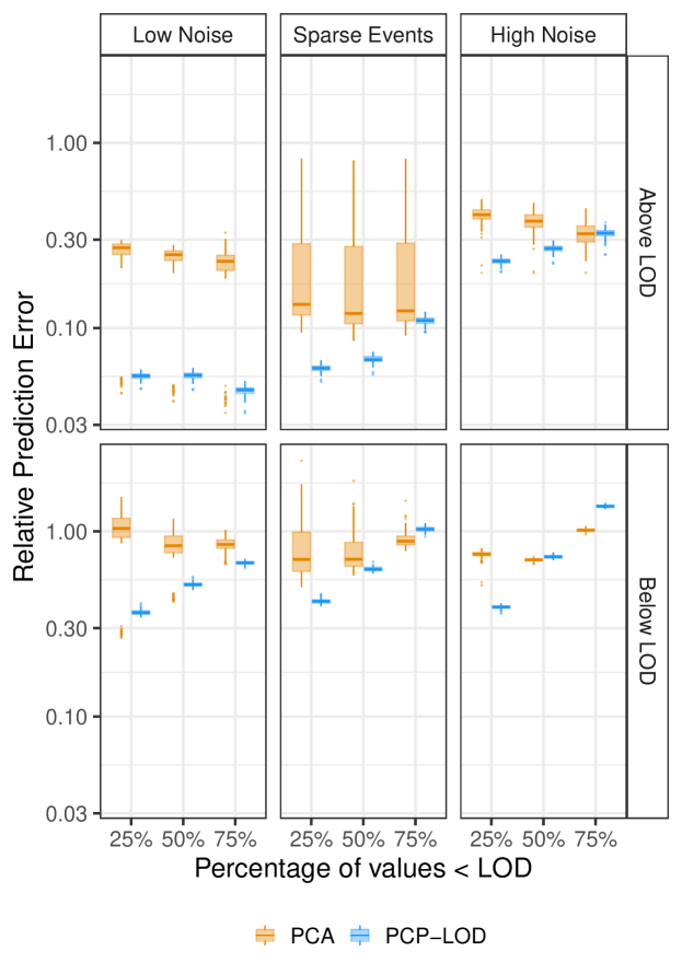
We ran PCP-LOD and PCA on all simulated datasets. PCP-LOD had lower relative prediction error across the majority of mixture sizes ( = 16 and 48), proportions LOD (25%, 50%, and 75%), and noise structures (low, high, and sparse). PCP-LOD outperformed PCA on all simulations with low noise, simulations with high noise with up to 50% LOD, and simulations with low noise and added sparse events with up to 50% LOD (Figure 2). Figures 2 and 3 present simulations where = 16; corresponding figures where = 48 are included in Supplemental Figures S1 and S2.


PCP-LOD was more affected by the proportion of data LOD, which can be seen in the larger step size between box plots in Figure 2. The decline in PCP-LOD predictive accuracy as the proportion of values LOD increased appears because of poorer performance on values LOD in high noise scenarios (Figure 3). Relative prediction error for values LOD was approximately constant for PCP-LOD and PCA. Supplemental Tables S1, S2, and S3 contain the median and inter-quartile range (IQR) of relative error for predicted values overall and stratified by LOD.
Next, we assessed the stability of the identified patterns using the SVD of the simulated data before noise or sparse events were added and compared this with the SVD of the matrix and of PCA results. Figure 4 depicts the relative prediction error comparing the left eigenvectors (comparable to scaled individual scores) of the PCP-LOD and PCA solutions with those of the simulated ‘truth.’ PCP-LOD’s median relative prediction error is generally lower than PCA’s for the larger mixture size and higher than PCA’s for the smaller mixture size. However, these patterns appear quite stable over increasing proportions of data LOD for both methods. PCP-LOD solutions achieved lower relative prediction error on chemical loadings (i.e., right eigenvectors) across all simulations (Supplemental Figure S3).
Across PCP-LOD solutions, between 2% and 10% of entries were non-sparse. We found decreasing sparsity as the proportion LOD increased, with 3% (IQR: 2%, 4%), 6% (IQR: 4%, 7%), and 7% (IQR: 3%, 8%) unique events, on average, found in simulations with 25%, 50%, and 75% LOD, respectively. For simulations that included sparse events in the noise structure, PCP-LOD correctly included 69% (IQR: 67%, 71%), 70% (IQR: 68%, 72%), and 65% (IQR: 62%, 67%) of sparse values in the matrix, on average for simulations with 25%, 50%, and 75% LOD, respectively.
4.2 Application
Thirty-four POPs were measured in the NHANES 2001–2002 cycle. Detection frequency is presented in Figure 5. Fourteen PCBs, four furans, and three dioxins were detected in 50% of samples. Exposure levels of POPs were all positively correlated (Figure 6(a)).


We applied PCP-LOD to identify underlying patterns of POP exposure and extreme exposure events that were not explained by these patterns without making a priori assumptions concerning the number of patterns or sparse events. PCP-LOD returned a low-rank matrix of rank three, which corresponds with three patterns of POP exposure in the matrix. Figure 6(b) depicts ’s correlation matrix along side the correlation matrix of the raw data (Figure 6(a)). By removing sparse events and residual noise, PCP-LOD increased the correlations between POPs. To characterize underlying patterns, we extracted principal components from the low-rank matrix using SVD.
The three components distinguished by PCP-LOD included one component of overall POP exposure, a component that separated dioxins and furans from PCBs, and a third component that separated higher molecular weight PCBs from lower molecular weight PCBs (Figure 7). The first component explained 79.4% of the variance in the low-rank matrix, the second explained 14.6%, and the third explained 6.0%.
PCP-LOD partitioned the variation that was unexplained by the low-rank structure into a sparse matrix of large outlying values and the remaining residuals. The matrix contained mostly zero values, with 5.7% of entries being non-sparse. Sparse observations were generally weakly correlated, with the absolute value of r 0.15 for 70% of Spearman correlations between sparse chemical exposure events. Table 1 summarizes the number of individuals with uniquely high or low exposure events. Figure 8 describes participant-specific sparse events. Most participants had no extreme exposures (44%) or only extremely low exposures (18%). Twenty-two percent had one high unique event on a single chemical, and 16% had between two and six high exposures across 21 chemicals left unexplained by the identified patterns.
| High Unique Events | |||||||||
| 0 | 1 | 2 | 3 | 4 | 5 | 6 | |||
| Low Unique Events | 0 | 439 | 141 | 41 | 11 | 5 | 0 | 1 | 638 |
| 1 | 147 | 46 | 30 | 13 | 5 | 1 | 0 | 242 | |
| 2 | 27 | 19 | 11 | 6 | 3 | 1 | 0 | 67 | |
| 3 | 8 | 11 | 9 | 8 | 2 | 1 | 1 | 40 | |
| 4 | 0 | 1 | 2 | 3 | 2 | 0 | 1 | 9 | |
| 5 | 0 | 0 | 0 | 1 | 0 | 0 | 1 | 2 | |
| 6 | 0 | 0 | 0 | 0 | 1 | 1 | 0 | 2 | |
| 621 | 218 | 93 | 42 | 18 | 4 | 4 | 1000 | ||
| Column sums of uniquely high events. | |||||||||
| Row sums of uniquely low events. | |||||||||

PCA conducted on the POP mixture chose three components that explained 80% of the variance and returned loadings and scores much the same as those from (results not shown). Using the three chosen components, PCA’s relative prediction error on values LOD was 0.30, similar to PCP-LOD’s relative error of 0.32 when comparing only with the original data. However, when including in the solution (), PCP-LOD’s relative error on values LOD was 0.07. This is more comparable to the PCA solution when including all 21 components, 0.06, which does not accomplish any dimension reduction.
5 Discussion
We propose PCP-LOD as a new approach to identify patterns—and extreme events left unexplained by patterns—underlying environmental chemical mixtures in the presence of values LOD. Our simulation studies highlighted three main advantages of PCP-LOD over PCA at identifying patterns in environmental mixtures: (1) reduced error in estimated patterns of exposure, (2) identification of extreme or unique events, and (3) improved estimation of values LOD.
Patterns identified by PCP-LOD are additionally more robust to noise and incomplete data than more traditional pattern identification methods because patterns in are not influenced by events in . PCP-LOD estimated the underlying low-rank structure of with lower relative error than PCA under all realistic simulation scenarios. PCA outperformed PCP-LOD for two error structures when 75% of the dataset was simulated as LOD. In this case, PCP-LOD used 25% to re-construct 75% of the data, and poorer performance was expected. However, it is unlikely that an environmental health researcher will face a chemical mixture with 75% of all values LOD. In our application to POPs detected in over 50% of measurements among NHANES participants, 76% of all observations were LOD. In the entire POP mixture of 34 chemicals, with five chemicals never detected, 52% of all observations were LOD. We observed the highest relative prediction error across all simulations for values LOD in simulated datasets. This held for PCA, as well, and applies to all methods to address censored or missing data.
In our simulations and application to NHANES data, we did not make use of the non-negativity constraint, as SVD returns solutions with negative values. However, we paired PCP-LOD with SVD to make results comparable with those of PCA. This is not a constraint of PCP-LOD, as it may be paired with various dimension reduction techniques. Because of the non-negativity constraint on the matrix, for example, PCP-LOD can be paired with NMF to provide results interpretable on an additive scale with a parts-based representation. [36].
The three components underlying the NHANES mixture distinguished by PCP-LOD represent one pattern of exposure to all POPs and two patterns grouped by known structural and toxicological properties. More than 90% of human exposure to PCBs, dioxins, and furans is through the food supply, mainly meat, dairy, and seafood [37, 38, 39]. Thus, the first component of comprehensive exposure may be interpreted as a dietary source of these POPs. The second component separated dioxins and furans, which are generally more toxic, from PCBs [40]. Accordingly, we can understand the second component as a measure of toxicity. The third component separated lower molecular weight PCBs from higher molecular weight PCBs, where larger numbers indicate more chlorine atoms and larger molecules. Higher chlorinated congeners tend to bioaccumulate more than lower chlorinated congeners [41, 42]. Depending on the research question, any or all of these components could be included in subsequent analyses with health outcomes.
In the original POP mixture, individuals with high values on any chemicals were likely to have high values on other chemicals, or equivalently, individuals with low values on any chemicals were likely to have low values on other chemicals. PCP-LOD captured this in a component representing overall mixture exposure. After removing the underlying patterns in the mixture described in , high (or low) exposure events on individual chemicals did not indicate high (or low) exposure to other chemicals, i.e., sparse events in were not highly correlated. About half (51%) of the unique low exposure events were LOD in the original mixture; these values LOD were not explained by overall low exposure or by the other identified patterns.
The ability to identify and separate extreme events is a unique feature offered by PCP-LOD and cannot be found in other methods. These unique or extreme events not captured in may themselves be risk factors (e.g., wildfires—unique events not explained by commonly recognized air pollution sources—for asthma emergency admissions)[43], or they may modify an association with one of the components (e.g., a Saharan dust episode might modify the association with traffic-related pollution) [44]. Next steps could entail including exposures along with identified patterns from in a health model with some form of penalization (e.g., lasso or elastic net).
While PCP-LOD addresses several drawbacks of existing methods, it does not overcome all limitations of pattern identification in environmental mixtures. First, in multi-pollutant exposures the ‘true’ originating mechanism is almost never known, thus PCP-LOD cannot provide the ‘correct’ answer. PCP-LOD, like other methods employed in our field, should be used in conjunction with subject area expertise. The interpretability of results relies on this expert knowledge. This limitation applies, however, to all methods to address research questions concerning patterns of environmental exposures. Second, including scores obtained from any dimension reduction technique paired with PCP-LOD in a health model ignores the uncertainty inherent in the solution selection, resulting in underestimated confidence intervals and, potentially, spurious results [3]. Third, some datasets will likely be high-dimensional, with a large number of correlated chemical measurements for each participant. In this situation, PCP-LOD still performs well, provided the rank of the target matrix is small enough compared to (e.g., , where is a constant) [23]. Additionally, our application findings should be interpreted in light of their limitations. First, as is the case when using chemical biomarkers, our study is susceptible to exposure measurement error. In a noisy setting, any method will exhibit an inaccuracy in the estimated left singular vectors, which is commensurate with the noise level. Nevertheless, even in this setting, the results produced by PCP-LOD are stable with respect to noise [23]. Second, our results may not be generalizable beyond the study population. While NHANES includes a nationally-representative sample of the general non-institutionalized US population [45], we did not account for the complex sampling design and weights of the study [46]. Thus, the PCP-LOD-identified patterns may represent sources or behaviors distinct to the participants.
PCP-LOD also has numerous strengths when compared with existing methods to identify exposure patterns in environmental mixtures, which require strong assumptions and have key limitations. As a consequence, their use has resulted in heterogeneous and inconsistent findings across studies [1]. Moreover, results from methods that are not generalizable or interpretable hinder their use in the design and development of regulations, policies, and targeted interventions. Original PCP has few assumptions, namely that is not sparse and that is not low-rank [19]. This is an appealing feature of a tool when the underlying truth is not known. PCP-LOD directly addresses several additional limitations of existing methods: (1) its solution is not necessarily orthogonal, allowing correlations between patterns, (2) its solution is non-negative, so patterns can exist in an interpretable space, (3) its parameters do not require tuning by the researcher, meaning that the choice of number of patterns in is not subjective, and (4) PCP-LOD is robust to extreme values because of the novel matrix.
To our knowledge, this work represents the first instance of decomposing the structure among chemicals in an additive manner. By separating the unique events from underlying patterns, PCP-LOD provides the opportunity to include extreme events in analyses, where they previously may have been suppressed or discarded. The theory-backed parameter selection and cross-validation enhances reproducibility of PCP-LOD, ensuring that two different research groups with the same dataset will identify the same optimal number of patterns. PCP-LOD may be employed when environmental epidemiologists have research questions concerning sources or behaviors leading to chemical exposure or patterns underlying exposure to multi-pollutant mixtures, especially when data are noisy, incomplete, or may contain extreme exposure events.
Acknowledgements
This work was partially supported by the National Institutes of Environmental Health (NIEHS) individual fellowship grant F31 ES030263, as well as PRIME R01 ES028805 and P30 ES009089.
6 Supplemental Materials
| 25% LOD | 50% LOD | 75% LOD | ||||||||
|---|---|---|---|---|---|---|---|---|---|---|
| Simulated Data | Method | |||||||||
| Low noise | PCA | 0.27 | 0.30 | 0.31 | 0.28 | 0.31 | 0.32 | 0.36 | 0.38 | 0.39 |
| PCP-LOD | 0.07 | 0.08 | 0.10 | 0.12 | 0.13 | 0.14 | 0.24 | 0.26 | 0.27 | |
| High noise | PCA | 0.40 | 0.43 | 0.45 | 0.40 | 0.42 | 0.45 | 0.55 | 0.57 | 0.59 |
| PCP-LOD | 0.24 | 0.30 | 0.37 | 0.35 | 0.38 | 0.42 | 0.63 | 0.67 | 0.71 | |
| Low noise | PCA | 0.15 | 0.21 | 0.31 | 0.19 | 0.23 | 0.33 | 0.35 | 0.37 | 0.44 |
| + sparse events | PCP-LOD | 0.08 | 0.09 | 0.12 | 0.15 | 0.16 | 0.17 | 0.36 | 0.38 | 0.40 |
| 25% LOD | 50% LOD | 75% LOD | ||||||||
|---|---|---|---|---|---|---|---|---|---|---|
| Simulated Data | Method | |||||||||
| Low noise | PCA | 0.25 | 0.27 | 0.29 | 0.23 | 0.25 | 0.26 | 0.21 | 0.23 | 0.25 |
| PCP-LOD | 0.06 | 0.07 | 0.09 | 0.06 | 0.07 | 0.08 | 0.05 | 0.05 | 0.07 | |
| High noise | PCA | 0.39 | 0.41 | 0.43 | 0.35 | 0.38 | 0.41 | 0.31 | 0.35 | 0.36 |
| PCP-LOD | 0.23 | 0.29 | 0.36 | 0.27 | 0.32 | 0.38 | 0.33 | 0.36 | 0.41 | |
| Low noise | PCA | 0.13 | 0.19 | 0.29 | 0.12 | 0.18 | 0.27 | 0.12 | 0.18 | 0.27 |
| + sparse events | PCP-LOD | 0.06 | 0.08 | 0.11 | 0.07 | 0.08 | 0.11 | 0.11 | 0.12 | 0.14 |
| 25% LOD | 50% LOD | 75% LOD | ||||||||
|---|---|---|---|---|---|---|---|---|---|---|
| Simulated Data | Method | |||||||||
| Low noise | PCA | 0.92 | 1.04 | 1.17 | 0.78 | 0.85 | 0.93 | 0.82 | 0.85 | 0.90 |
| PCP-LOD | 0.36 | 0.37 | 0.38 | 0.51 | 0.52 | 0.54 | 0.68 | 0.70 | 0.73 | |
| High noise | PCA | 0.67 | 0.72 | 0.75 | 0.64 | 0.67 | 0.70 | 0.99 | 1.01 | 1.03 |
| PCP-LOD | 0.39 | 0.45 | 0.52 | 0.66 | 0.70 | 0.73 | 1.10 | 1.25 | 1.36 | |
| Low noise | PCA | 0.65 | 0.77 | 1.03 | 0.67 | 0.74 | 0.88 | 0.84 | 0.89 | 0.95 |
| + sparse events | PCP-LOD | 0.41 | 0.42 | 0.44 | 0.60 | 0.62 | 0.63 | 0.88 | 0.97 | 1.03 |


References
- Gibson et al. [2019a] Elizabeth A Gibson, Jeff Goldsmith, and Marianthi-Anna Kioumourtzoglou. Complex mixtures, complex analyses: an emphasis on interpretable results. Current environmental health reports, pages 1–9, 2019a.
- Pang et al. [2016] Yuanjie Pang, Roger D Peng, Miranda R Jones, Kevin A Francesconi, Walter Goessler, Barbara V Howard, Jason G Umans, Lyle G Best, Eliseo Guallar, Wendy S Post, et al. Metal mixtures in urban and rural populations in the US: The Multi-Ethnic Study of Atherosclerosis and the Strong Heart Study. Environmental research, 147:356–364, 2016.
- Kioumourtzoglou et al. [2014] Marianthi-Anna Kioumourtzoglou, Brent A Coull, Francesca Dominici, Petros Koutrakis, Joel Schwartz, and Helen Suh. The impact of source contribution uncertainty on the effects of source-specific PM2.5 on hospital admissions: A case study in Boston, MA. Journal of Exposure Science and Environmental Epidemiology, 24(4):365–371, 2014.
- Gibson et al. [2019b] Elizabeth A Gibson, Yanelli Nunez, Ahlam Abuawad, Ami R Zota, Stefano Renzetti, Katrina L Devick, Chris Gennings, Jeff Goldsmith, Brent A Coull, and Marianthi-Anna Kioumourtzoglou. An overview of methods to address distinct research questions on environmental mixtures: an application to persistent organic pollutants and leukocyte telomere length. Environmental Health, 18(1):76, 2019b.
- Robinson et al. [2018] Oliver Robinson, Ibon Tamayo, Montserrat De Castro, Antonia Valentin, Lise Giorgis-Allemand, Norun Hjertager Krog, Gunn Marit Aasvang, Albert Ambros, Ferran Ballester, Pippa Bird, et al. The urban exposome during pregnancy and its socioeconomic determinants. Environmental health perspectives, 126(7):077005, 2018.
- Manzano-León et al. [2015] Natalia Manzano-León, Jesús Serrano-Lomelin, Brisa N Sánchez, Raúl Quintana-Belmares, Elizabeth Vega, Inés Vázquez-López, Leonora Rojas-Bracho, Maria Tania López-Villegas, Felipe Vadillo-Ortega, Andrea De Vizcaya Ruiz, et al. Tnf and il-6 responses to particulate matter in vitro: Variation according to pm size, season, and polycyclic aromatic hydrocarbon and soil content. Environmental health perspectives, 124(4):406–412, 2015.
- Jolliffe [1986] Ian T Jolliffe. Principal components in regression analysis. In Principal component analysis, pages 129–155. Springer, 1986.
- Jolliffe and Cadima [2016] Ian T Jolliffe and Jorge Cadima. Principal component analysis: a review and recent developments. Philosophical Transactions of the Royal Society A: Mathematical, Physical and Engineering Sciences, 374(2065):20150202, 2016.
- Lever et al. [2017] Jake Lever, Martin Krzywinski, and Naomi Altman. Points of significance: Principal component analysis, 2017.
- Friedman et al. [2001] Jerome Friedman, Trevor Hastie, and Robert Tibshirani. The elements of statistical learning, volume 1. Springer series in statistics New York, NY, USA:, 2001.
- Wold et al. [1987] Svante Wold, Kim Esbensen, and Paul Geladi. Principal component analysis. Chemometrics and intelligent laboratory systems, 2(1-3):37–52, 1987.
- Gull and Daniell [1978] Stephen F Gull and Geoff J Daniell. Image reconstruction from incomplete and noisy data. Nature, 272(5655):686–690, 1978.
- Helsel [2005] Dennis R Helsel. More than obvious: better methods for interpreting nondetect data. Environmental science & technology, 39(20):419A–423A, 2005.
- Helsel et al. [2005] Dennis R Helsel et al. Nondetects and data analysis. Statistics for censored environmental data. Wiley-Interscience, 2005.
- EPA [2000] U.S. EPA. Guidance for data quality assessment. practical methods for data analysis. EPA QA/G-9, QA00 version. Washington, DC, U.S. Environmental Protection Agency, Office of Environmental Information., 2000. [https://www.epa.gov/sites/production/files/2015-06/documents/g9-final.pdf; accessed 29-April-2021].
- Barr et al. [2006] Dana B Barr, Doug Landsittel, Marcia Nishioka, Kent Thomas, Brian Curwin, James Raymer, Kirby C Donnelly, Linda McCauley, and P Barry Ryan. A survey of laboratory and statistical issues related to farmworker exposure studies. Environmental health perspectives, 114(6):961–968, 2006.
- Hornung and Reed [1990] Richard W Hornung and Laurence D Reed. Estimation of average concentration in the presence of nondetectable values. Applied occupational and environmental hygiene, 5(1):46–51, 1990.
- Helsel [1990] Dennis R Helsel. Less than obvious-statistical treatment of data below the detection limit. Environmental science & technology, 24(12):1766–1774, 1990.
- Candès et al. [2011] Emmanuel J Candès, Xiaodong Li, Yi Ma, and John Wright. Robust principal component analysis? Journal of the ACM (JACM), 58(3):1–37, 2011.
- Zhang et al. [2021] Junhui Zhang, Jingkai Yan, and John Wright. Square root principal component pursuit: Tuning-free noisy robust matrix recovery. arXiv preprint arXiv:2106.09211, 2021.
- Netrapalli et al. [2014] Praneeth Netrapalli, UN Niranjan, Sujay Sanghavi, Animashree Anandkumar, and Prateek Jain. Non-convex robust pca. arXiv preprint arXiv:1410.7660, 2014.
- Chen et al. [2020] Yuxin Chen, Jianqing Fan, Cong Ma, and Yuling Yan. Bridging convex and nonconvex optimization in robust pca: Noise, outliers, and missing data. arXiv preprint arXiv:2001.05484, 2020.
- Zhou et al. [2010] Zihan Zhou, Xiaodong Li, John Wright, Emmanuel Candes, and Yi Ma. Stable principal component pursuit. In Information Theory Proceedings (ISIT), 2010 IEEE International Symposium on, pages 1518–1522. IEEE, 2010.
- Chen and Wainwright [2015] Yudong Chen and Martin J Wainwright. Fast low-rank estimation by projected gradient descent: General statistical and algorithmic guarantees. arXiv preprint arXiv:1509.03025, 2015.
- Chandrasekaran et al. [2011] Venkat Chandrasekaran, Sujay Sanghavi, Pablo A Parrilo, and Alan S Willsky. Rank-sparsity incoherence for matrix decomposition. SIAM Journal on Optimization, 21(2):572–596, 2011.
- Lin et al. [2010] Zhouchen Lin, Minming Chen, and Yi Ma. The augmented lagrange multiplier method for exact recovery of corrupted low-rank matrices. arXiv preprint arXiv:1009.5055, 2010.
- Boyd et al. [2004] Stephen Boyd, Stephen P Boyd, and Lieven Vandenberghe. Convex optimization. Cambridge university press, 2004.
- Wright and Ma [2021] John Wright and Yi Ma. High-Dimensional Data Analysis with Low-Dimensional Models: Principles, Computation, and Applications. Cambridge University Press, 2021.
- Zipf et al. [2013] George Zipf, Michele Chiappa, Kathryn S Porter, Yechiam Ostchega, Brenda G Lewis, and Jennifer Dostal. Health and nutrition examination survey plan and operations, 1999-2010. Vital and Health Statistics, 1(56), 2013.
- CDC [2002] CDC. Laboratory procedure manual: Pcbs and persistent pesticides in serum. 2001—2002. https://www.cdc.gov/nchs/data/nhanes/nhanes_01_02/l28poc_b_met_pcb_pesticides.pdf, 2002. [Online; accessed 28-November-2018].
- CDC [2002] CDC. Laboratory procedure manual: Pcdds, pcdfs, and cpcbs in serum. 2001—2002. https://www.cdc.gov/nchs/data/nhanes/nhanes_01_02/l28poc_b_met_dioxin_pcb.pdf, 2002. [Online; accessed 28-November-2018].
- Akins et al. [1989] James R Akins, Kay Waldrep, and John T Bernert Jr. The estimation of total serum lipids by a completely enzymatic ‘summation’method. Clinica chimica acta, 184(3):219–226, 1989.
- Diana and Tommasi [2002] Giancarlo Diana and Chiara Tommasi. Cross-validation methods in principal component analysis: a comparison. Statistical Methods and Applications, 11(1):71–82, 2002.
- Krzanowski [1987] WJ Krzanowski. Cross-validation in principal component analysis. Biometrics, pages 575–584, 1987.
- R Core Team [2019] R Core Team. R: A Language and Environment for Statistical Computing. R Foundation for Statistical Computing, Vienna, Austria, 2019. URL https://www.R-project.org/.
- Lee and Seung [1999] Daniel D Lee and H Sebastian Seung. Learning the parts of objects by non-negative matrix factorization. Nature, 401(6755):788–791, 1999.
- Faroon and Olson [2000] Obaid Faroon and James N Olson. Toxicological profile for polychlorinated biphenyls (pcbs). 2000.
- Organization et al. [1999] World Health Organization et al. Dioxins and their effects on human health. In Dioxins and their effects on human health. 1999.
- Loganathan and Masunaga [2020] Bommanna G Loganathan and Shigeki Masunaga. Pcbs, dioxins, and furans: human exposure and health effects. In Handbook of toxicology of chemical warfare agents, pages 267–278. Elsevier, 2020.
- on the Evaluation of Carcinogenic Risks to Humans et al. [2012] IARC Working Group on the Evaluation of Carcinogenic Risks to Humans et al. Chemical agents and related occupations. IARC monographs on the evaluation of carcinogenic risks to humans, 100:225–248, 2012.
- Steele et al. [1986] G Steele, P Stehr-Green, and E Welty. Estimates of the biologic half-life of polychlorinated biphenyls in human serum. New England journal of medicine (USA), 1986.
- Hopf et al. [2009] Nancy B Hopf, Avima M Ruder, and Paul Succop. Background levels of polychlorinated biphenyls in the us population. Science of the total environment, 407(24):6109–6119, 2009.
- Delfino et al. [2008] Ralph J Delfino, Sean Brummel, Jun Wu, Hal Stern, Bart Ostro, Michael Lipsett, Arthur Winer, Donald H Street, Lixia Zhang, Thomas Tjoa, et al. The relationship of respiratory and cardiovascular hospital admissions to the southern california wildfires of 2003. Occupational and environmental medicine, 66(3):189–97, 2008.
- Karanasiou et al. [2012] A Karanasiou, N Moreno, T Moreno, M Viana, F De Leeuw, and X Querol. Health effects from sahara dust episodes in europe: literature review and research gaps. Environment international, 47:107–114, 2012.
- Johnson et al. [2013] Clifford L Johnson, Ryne Paulose-Ram, Cynthia L Ogden, Margaret D Carroll, Deanna Kruszan-Moran, Sylvia M Dohrmann, and Lester R Curtin. National health and nutrition examination survey. analytic guidelines, 1999-2010. 2013.
- Curtin et al. [2012] Lester R Curtin, Leyla K Mohadjer, Sylvia M Dohrmann, Jill M Montaquila, Deanna Kruszan-Moran, Lisa B Mirel, Margaret D Carroll, Rosemarie Hirsch, Susan Schober, and Clifford L Johnson. The national health and nutrition examination survey: Sample design, 1999-2006. Vital and health statistics. Series 2, Data evaluation and methods research, (155):1–39, 2012.