WUCG-22-11
Primordial black holes from Higgs inflation with a Gauss-Bonnet coupling
Abstract
Primordial black holes (PBHs) can be the source for all or a part of today’s dark matter density. Inflation provides a mechanism for generating the seeds of PBHs in the presence of a temporal period where the velocity of an inflaton field rapidly decreases toward 0. We compute the primordial power spectra of curvature perturbations generated during Gauss-Bonnet (GB) corrected Higgs inflation in which the inflaton field has not only a nonminimal coupling to gravity but also a GB coupling. For a scalar-GB coupling exhibiting a rapid change during inflation, we show that curvature perturbations are sufficiently enhanced by the appearance of an effective potential containing the structures of plateau-type, bump-type, and their intermediate type. We find that there are parameter spaces in which PBHs can constitute all dark matter for these three types of . In particular, models with bump- and intermediate-types give rise to the primordial scalar and tensor power spectra consistent with the recent Planck data on scales relevant to the observations of cosmic microwave background. This property is attributed to the fact that the number of e-foldings acquired around the bump region of can be as small as a few, in contrast to the plateau-type where typically exceeds the order of 10.
I Introduction
If there were over-density regions in the early universe, primordial black holes (PBHs) may form as a result of the gravitational collapse during the radiation-dominated epoch Zel’dovich and Novikov (1967); Hawking (1971); Carr and Hawking (1974). Unlike astrophysical black holes, the PBHs can have a wide range of masses and can be the source for all or a part of dark matter (DM) Chapline (1975); Meszaros (1975) (see Refs. Khlopov (2010); Sasaki et al. (2018); Carr and Kuhnel (2020); Green and Kavanagh (2021); Villanueva-Domingo et al. (2021); Carr and Kuhnel (2022); Escrivà et al. (2022); Karam et al. (2022) for recent reviews). Although PBHs have not been observationally discovered yet, the detection of gravitational waves from binary black holes Abbott et al. (2016, 2019, 2021a, 2021b) suggested a possibility that they may arise from non-stellar origins Bird et al. (2016); Sasaki et al. (2016); Clesse and García-Bellido (2017); Wang et al. (2018). In addition, PBHs have been also considered as possible seeds of supermassive black holes in the center of galaxies Bean and Magueijo (2002). Various observations have given the upper limit to their abundance as a function of mass . In particular, the mass window in which all DM can be explained by PBHs exists in the range , where is a solar mass (see Ref. Carr et al. (2021) for a recent study).
Inflation can provide a possible framework for generating the seed of PBHs on scales smaller than the observed cosmic microwave background (CMB) temperature anisotropies Ivanov et al. (1994); Garcia-Bellido et al. (1996); Bullock and Primack (1997); Yokoyama (1997, 1998); Kawasaki et al. (1998, 2006); Kohri et al. (2008); Saito et al. (2008); Bugaev and Klimai (2008); Alabidi and Kohri (2009); Drees and Erfani (2011, 2012); Martin et al. (2013); Kohri et al. (2013); Kawasaki et al. (2013); Clesse and García-Bellido (2015); Kawasaki and Tada (2016); Kawasaki et al. (2016); Pi et al. (2018); Garcia-Bellido and Ruiz Morales (2017); Kannike et al. (2017); Germani and Prokopec (2017); Ando et al. (2018); Ezquiaga et al. (2018); Motohashi and Hu (2017); Di and Gong (2018); Ballesteros and Taoso (2018); Garcia-Bellido et al. (2017); Hertzberg and Yamada (2018); Inomata et al. (2018); Cai et al. (2018a); Drees and Xu (2021); Atal et al. (2019, 2020); Mishra and Sahni (2020); Cheong et al. (2021); Fu et al. (2019); Dalianis et al. (2020); Ashoorioon et al. (2021); Lin et al. (2020); Yi et al. (2021); Palma et al. (2020); Braglia et al. (2020); Kefala et al. (2021); Ballesteros et al. (2020); Aldabergenov et al. (2020, 2021); Inomata et al. (2021, 2022a); Dalianis et al. (2021); Cai et al. (2022a); Lin et al. (2021); Kawai and Kim (2021a); Zhang (2022); Ahmed et al. (2022); Cai et al. (2022b); Pi and Wang (2022); Cheong et al. (2022); Kawai and Kim (2022). If there is an intermediate stage in which the velocity of an inflaton field rapidly decreases toward 0 during inflation, it is possible to enhance curvature perturbations at particular scales. In the presence of an inflection point in the inflaton potential around which the derivative is close to 0, the field velocity decreases as in the ultra-slow-roll (USR) regime, where is a scale factor Garcia-Bellido and Ruiz Morales (2017); Kannike et al. (2017); Germani and Prokopec (2017); Ezquiaga et al. (2018); Motohashi and Hu (2017); Di and Gong (2018); Ballesteros and Taoso (2018); Hertzberg and Yamada (2018); Drees and Xu (2021); Ballesteros et al. (2020). In many of these models, we require a tuning of model parameters to generate a plateau region of the potential. Moreover, if the number of e-foldings acquired in the USR regime exceeds the order 10, the scalar spectral index on CMB scales tends to be inconsistent with the value constrained by the Planck data Akrami et al. (2020).
There are also models containing one or more bumps/dips or steps in the potential Atal et al. (2019, 2020); Mishra and Sahni (2020); Kefala et al. (2021); Inomata et al. (2021, 2022a); Dalianis et al. (2021); Cai et al. (2022a, b); Pi and Wang (2022). In this case, the scalar field rapidly loses its kinetic energy around them, resulting in a strong enhancement of curvature perturbations. It is also known that oscillating features can appear in the scalar power spectrum especially for the step-type potential. One advantage of these models is that the number of e-foldings during transition can be as small as the order 1. This allows a possibility for the compatibility of models with the observed values of and tensor-to-scalar ratio . There are also multi-field inflationary models leading to the enhancement of curvature perturbations at particular scales Yokoyama (1997); Garcia-Bellido et al. (1996); Kawasaki et al. (1998, 2013); Kohri et al. (2013); Ando et al. (2018); Aldabergenov et al. (2020, 2021); Palma et al. (2020); Braglia et al. (2020); Cheong et al. (2022); Kawai and Kim (2022). In this case, we need to address whether the presence of entropy perturbations does not contradict with CMB constraints on the isocurvature mode. The possibility for producing the seed of PBHs during preheating after inflation was also discussed in Refs. Green and Malik (2001); Bassett and Tsujikawa (2001); Suyama et al. (2005); Martin et al. (2020).
One of the advantages of PBHs as DM is that the origin of DM can be explained within the framework of Standard Model (SM) of particle physics. A minimal model of inflation without introducing additional scalar degrees of freedom to those appearing in SM is known as Higgs inflation, in which the Higgs field is nonminimally coupled to gravity Bezrukov and Shaposhnikov (2008); Bezrukov et al. (2009, 2011) (see Refs. Futamase and Maeda (1989); Fakir and Unruh (1990) for early related works). Indeed, this model is perfectly consistent with observational bounds on and constrained by the CMB data Komatsu and Futamase (1999); Tsujikawa and Gumjudpai (2004); Linde et al. (2011); Ade et al. (2014); Tsujikawa et al. (2013). If we allow the runnings of Higgs self-coupling and nonminimal coupling , then it is possible to have an inflection point in the Higgs potential. This gives rise to a plateau region in which the enhancement of curvature perturbations occurs to generate the seed of PBHs Ezquiaga et al. (2018); Drees and Xu (2021); Yi et al. (2021); Lin et al. (2021). In this scenario the typical number of e-foldings acquired during the USR regime is of order 10, which results in the values of CMB observables deviating from those in standard Higgs inflation. The model can be consistent with the current CMB observations, but it is typically outside the contour constrained by the Planck data Ezquiaga et al. (2018).
Recently, Kawai and Kim Kawai and Kim (2021a) proposed a single-field inflationary scenario in which the inflaton field is coupled to a Gauss-Bonnet (GB) curvature invariant of the form . A scalar-field dependent GB coupling can give rise to an inflection point in an effective potential of the inflaton. On the other hand, we have to caution that a large contribution from the scalar-GB coupling to the inflaton energy density modifies the primordial scalar power spectrum on CMB scales Hwang and Noh (2005); Guo et al. (2007); Satoh and Soda (2008); Guo and Schwarz (2009, 2010); Kawai and Kim (2021b). Moreover, the scalar-GB coupling leads to the propagation speeds of scalar and tensor perturbations different from the speed of light Kobayashi et al. (2011); Kase and Tsujikawa (2019). Since the Laplacian instabilities associated with negative squared propagation speeds may arise, we need to make sure whether the stability conditions are not violated during inflation.
In Ref. Kawai and Kim (2021a), the scalar-GB coupling was proposed to generate the seed of PBHs around the inflection point . Since approaches constants in the two asymptotic regimes and , the scalar-GB coupling is important only in the vicinity of . A temporal USR region can arise from the balance between the GB term and the scalar potential. The enhancement of curvature perturbations in such a transient epoch was studied for natural inflation Kawai and Kim (2021a) and for -attractor Zhang (2022). In these papers, the authors mostly focused on the USR regime realized by a plateau-type effective potential. In this case, the CMB observables are subject to modifications by the presence of a plateau-region with the number of e-foldings of order 10. Hence it is nontrivial to produce the large amplitude of primordial scalar perturbations responsible for the seed of PBHs, while satisfying CMB constraints on and .
In this paper, we will address this issue in Higgs inflation with a scalar-GB coupling mentioned above. We will not incorporate the runnings of Higgs and nonminimal couplings to focus on effects of the scalar-GB coupling on the background and perturbations. We show that, besides the plateau-type effective potential, it is possible to realize a bump- or step-type effective potential. In this latter case, the field velocity around decreases faster in comparison to the USR regime with a smaller number of e-foldings of order 1. The primordial scalar power spectrum can also have a sharp feature with a peak amplitude enhanced by a factor of . In such cases, PBHs can be the source for all DM in the mass range . Moreover, the bump-type effective potential can give rise to the values of and inside the observational contour constrained by the Planck CMB data. There are also intermediate-type potentials between plateau- and bump-types consistent with the CMB constraints, while generating the seed of PBHs. Thus, our inflationary scenario provides a versatile possibility for realizing various shapes of the effective scalar potential. We note that each shape of potentials was discussed separately in different contexts in the literature.
This paper is organized as follows. In Sec. II, we obtain the background equations of motion in Higgs inflation with a scalar-GB coupling and revisit the scalar and tensor power spectra generated in slow-roll Higgs inflation with . In Sec. III, we derive an effective potential of the inflaton field and classify it into three classes: (1) plateau-type, (2) bump-type, and (3) intermediate-type. In Sec. IV, we compute the primordial scalar power spectra for three sets of model parameters with which there are neither ghost nor Laplacian instabilities. We show that the bump-type is favored over the plateau-type for the consistency with CMB observables. In Sec. V, we calculate the PBH abundance relative to the relic DM density and show that our model produces a sufficient amount of PBHs that can be the source for all DM. Sec. VI is devoted to conclusions. Throughout the paper, we use the natural units ().
II Inflationary model with a Gauss-Bonnet term
We begin with theories given by the action
| (1) |
where is a determinant of the metric tensor , is the reduced Planck mass, is a nonminimal coupling constant, is a scalar field with the covariant derivative operator , and is the Ricci scalar. The scalar field has a potential of the form
| (2) |
where is a positive coupling constant. The dynamics of nonminimally coupled inflation with the potential (2) was originally addressed in Refs. Futamase and Maeda (1989); Fakir and Unruh (1990) (see also Refs. Salopek et al. (1989); Makino and Sasaki (1991); Kaiser (1995); Komatsu and Futamase (1999); Tsujikawa and Gumjudpai (2004)). It can also accommodate the Higgs potential in the large field regime , where GeV Bezrukov and Shaposhnikov (2008); Bezrukov et al. (2009, 2011). Provided that the nonminimal coupling is in the range
| (3) |
the self-coupling of order can be consistent with the amplitude of observed CMB temperature anisotropies333If we consider quantum corrections arising from the renormalization group running of the standard model, the Higgs self-coupling can be much smaller than 0.01 or even negative at inflationary energy scales De Simone et al. (2009); Hamada et al. (2014, 2015); Bezrukov et al. (2015, 2018). In this paper, we do not consider the runnings of coupling constants or ..
The scalar field is coupled to a GB curvature invariant defined by
| (4) |
with a -dependent coupling function , where and are the Ricci and Riemann tensors, respectively. The action (1) belongs to a subclass of Horndeski theories with second-order field equations of motion Horndeski (1974); Kobayashi et al. (2011); Deffayet et al. (2011); Charmousis et al. (2012) (see Appendix. A). In this case, there is only one propagating scalar degree of freedom besides two tensor polarizations. As we will study in Sec. III, it is possible to enhance scalar perturbations at particular scales for a specific choice of . The action (1) corresponds to Higgs inflation corrected by the Higgs-GB coupling. This allows a possibility for generating the seed of PBHs as the source for all DM within the framework of SM of particle physics.
We note that the limit in the action (1) with the potential of natural inflation corresponds to the model studied by Kawai and Kim Kawai and Kim (2021a). In our model, the basic mechanism for the generation of seeds of PBHs is similar to that advocated in Ref. Kawai and Kim (2021a). However, natural inflation is in tension with the observation of CMB temperature anisotropies Akrami et al. (2020). Instead, we would like to construct an explicit inflationary model consistent with CMB observations, while enhancing curvature perturbations on scales relevant to PBHs. As we will show later, this is indeed possible for Higgs inflation with in the presence of the scalar-GB coupling.
For the background, we consider a spatially flat Friedmann-Lemaître-Robertson-Walker (FLRW) line element given by
| (5) |
where is a time-dependent scale factor. On this background, the Friedmann and scalar-field equations of motion are
| (6) | |||
| (7) |
where a dot represents a derivative with respect to , is the Hubble expansion rate, and we use the notations and . Taking the time derivative of Eq. (6) and using Eq. (7), we obtain the closed-form differential equations
| (8) | |||
| (9) |
where
| (10) | |||||
| (11) |
Notice that is an effective potential of the scalar field. Numerically, we solve Eqs. (8) and (9) for and with the initial conditions of , , and consistent with the Hamiltonian constraint (6).
II.1 Linear perturbations and stability conditions
To study the evolution of cosmological perturbations during inflation, we consider a perturbed line element containing scalar perturbations , , and tensor perturbations as
| (12) |
In full Horndeski theories including the action (1) as a special case, the linear perturbation equations of motion were already derived in the literature Kobayashi et al. (2011). On using the Hamiltonian and momentum constraints to eliminate and and integrating the action (1) by parts, the second-order action of scalar perturbations is given by Kobayashi et al. (2011); De Felice and Tsujikawa (2011a); Kawai and Kim (2021b)
| (13) |
where
| (14) |
with
| (15) | |||
| (16) |
In the tensor sector, the reduced action is of the form
| (17) |
where and are defined in Eq. (15). To avoid the ghost and Laplacian instabilities of scalar and tensor perturbations, we require the following conditions
| (18) |
On using the background Eq. (6), we can express and in the forms
| (19) |
Provided that decreases during inflation in the region , we have for . In such cases, both and are positive and hence the ghost instabilities are absent. In the absence of the scalar-GB coupling, both and are equivalent to 1. However, the deviations of and from 1 arise in theories with , so we need to numerically compute and for a given coupling to ensure the absence of Laplacian instabilities.
II.2 Higgs slow-roll inflation with
We briefly revisit the background dynamics and perturbation spectra generated during Higgs slow-roll inflation for . From Eqs. (6) and (9), we have
| (20) | |||
| (21) |
Let us consider the large coupling regime with and . During slow-roll inflation, the dominant term in Eq. (20) is the potential , while the dominant contributions to Eq. (21) are second and fourth terms. Then, Eqs. (20) and (21) approximately reduce to
| (22) |
The field value at the end of inflation is determined by the condition . Using the two equations in (22), we have and hence . The number of e-foldings counted backward from the end of inflation can be estimated as
| (23) |
where we exploited Eq. (22) in the second approximate equality. For , we obtain the simple relation .
For perturbations deep inside the Hubble radius (with the wavenumber ), they are initially in the Bunch-Davies vacuum state. On the inflationary background, and approach constants after the sound horizon crossing. The power spectra of scalar and tensor perturbations generated during the quasi de Sitter period are given, respectively, by Kobayashi et al. (2011)
| (24) |
In theories with , we have and hence both and should be evaluated at .
Since and in the regimes and , the power spectra (24) reduce to
| (25) | |||
| (26) |
where we used the approximate background Eq. (22). We note that the subscript is omitted in Eqs. (25) and (26). Then, we obtain the scalar spectral index and the tensor-to-scalar ratio , as
| (27) | |||||
| (28) |
Taking for scales relevant to the observed CMB temperature anisotropies, we obtain and . These values are consistent with the bounds (68 % CL) and (95 % CL) constrained by the Planck 2018 data Akrami et al. (2020). The Planck normalization with gives the constraint . If , then .
The above results are valid for slow-roll inflation with . In the presence of the scalar-GB coupling, the background dynamics and perturbation spectra are subject to modifications. In subsequent sections, we will address this issue along with the problem of generating the source for PBHs.
III Effective potentials with plateau and bump
Let us proceed to the case in which the scalar-GB coupling is present. If is a smooth function whose time variation is small during inflation, the inflaton field can slowly evolve along the potential. In such a case, the primordial power spectra of scalar and tensor perturbations are given by Eq. (24). Since is proportional to , a smaller inflaton velocity generally leads to a larger amplitude of . In the context of slow-roll inflation, however, this enhancement of is limited by a small time variation of .
If the scalar-GB coupling generates a period in which the field velocity temporally approaches 0, it is possible to realize the large enhancement of for scales smaller than those of the observed CMB temperature anisotropies. One possible choice of is a dilatonic coupling of the form Gross and Sloan (1987); Metsaev and Tseytlin (1987); Gasperini et al. (1997); Kawai et al. (1998); Cartier et al. (2001); Calcagni et al. (2005); Guo et al. (2007). However, this type of continuously varying functions affects not only the scalar perturbation on particular scales but also that on other scales including CMB. Moreover, it can happen that the dominance of the scalar-GB coupling over the potential and nonminimal couplings leads to the violation of stability conditions (18).
Instead, we consider the step-like coupling given by Kawai and Kim (2021a); Zhang (2022); Khan and Yogesh (2022)
| (29) |
where , , and are constants. Around the field value , this coupling rapidly changes from the asymptotic constant (for ) to the other asymptotic constant (for ). Since the GB curvature invariant is a topological term, the scalar-GB coupling does not affect the cosmological dynamics in the two asymptotic regimes with constant . Provided that is in the range , where is the field value about 60 e-foldings before the end of inflation (with the field value ), it should be possible to enhance the scalar power spectrum for scales smaller than those of observed CMB temperature anisotropies. In Sec. IV, we will study whether the sufficient generation of seeds for PBHs is possible, while satisfying observational constraints on and on CMB scales.
Provided that the field kinetic term is sufficiently small during inflation, we can ignore the -dependent terms in Eq. (10). Then, the -derivative of the effective potential is approximately given by
| (30) |
From Eq. (6), the Hubble parameter is approximately given by
| (31) |
Substituting Eq. (31) into Eq. (30) and integrating it with respect to , the effective potential can be numerically known as a function of .
In the following, we classify the effective potential into three classes: (1) plateau-type, (2) bump-type, and (3) intermediate-type. The set 1, 2, 3 model parameters shown in Table 1 are the typical examples of plateau-, bump-, and intermediate-types, respectively. The nonminimal coupling constant is fixed to be in all cases.
Since PBHs are treated as the main component of DM in this paper, we consider the PBH mass range . This gives a constraint on the value of . The two constants and determine the types of mentioned above. Instead of the parameter , we will use the combination
| (32) |
which appears later in Eq. (36). The values of are chosen to be close or not far away from the right hand side (RHS) of Eq. (36), see the last two columns in Table 1. The Higgs self-coupling is determined by the observed amplitude of primordial curvature perturbations on CMB scales. As we see in Table 1, is of order 0.01 for three sets of model parameters.
| \addstackgap [.5] | RHS of Eq. (36) | |||||
|---|---|---|---|---|---|---|
| \addstackgap [.5] Set 1 | 5000 | 0.0244211 | 0.0380 | 1000 | 1.564709 | 1.556127 |
| \addstackgap [.5] Set 2 | 5000 | 0.0110810 | 0.0760 | 5000 | 0.249909 | 0.176768 |
| \addstackgap [.5] Set 3 | 5000 | 0.0152511 | 0.0600 | 1600 | 0.376125 | 0.366512 |
III.1 Plateau type
Thanks to the existence of the scalar-GB coupling, there is a stationary fixed point at which vanishes Kawai and Kim (2021a). From Eq. (30) with Eq. (31), there is the following relation
| (33) |
This is known as the USR regime in which the scalar-field equation (9) reduces to Garcia-Bellido and Ruiz Morales (2017); Kannike et al. (2017); Germani and Prokopec (2017); Motohashi and Hu (2017)
| (34) |
The solution to this equation is given by
| (35) |
where is the number of e-foldings counted forward. Hence rapidly decreases toward 0 in the USR regime.
Setting for the coupling (29), the moment at which vanishes coincides with the instant at transition of . For the potential , the condition (33) translates to
| (36) |
which gives a constraint between and . During the USR regime, the variation of the scalar field is of order . On using Eqs. (22) and (35), we can estimate the order of as
| (37) |
where is the number of e-foldings acquired during the USR phase.
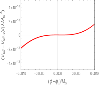
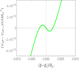
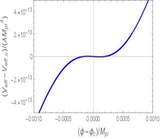
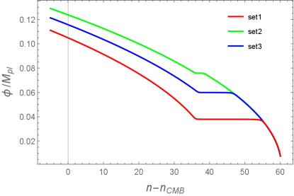
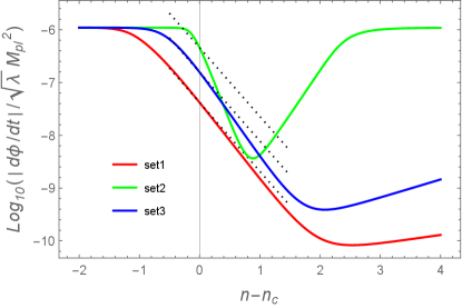
In the left panel of Fig. 1, we plot in the vicinity of for the Set 1 model parameters given in Table 1. In this case, is chosen to be close to the RHS of Eq. (36). There is a plateau of in the region , where . In the left panel of Fig. 2, we show the evolution of versus the number of e-foldings for the parameter Set 1 as a red line. The field value at the end of inflation is numerically derived by the condition , which gives .
The initial field value for realizing the total number of e-foldings by the end of inflation corresponds to (at which ). In this case, the first slow-roll stage of inflation is followed by the USR period starting at . After the inflaton approaches the plateau of around , the field derivative rapidly decreases as , see the right panel of Fig. 2. For the model parameters of Set 1, the number of e-foldings acquired during the USR epoch is 18.6. Finally, the scalar field exits from the USR regime, after which starts to increase.
As the plateau region of gets wider, the number of e-foldings acquired during the USR phase tends to be larger. For exceeding the order 10, the CMB observables like and are subject to modifications in comparison to those derived for . We will discuss this issue in Sec. IV.
III.2 Bump type
For the plateau-type effective potential, the scalar-GB coupling balances the contributions arising from the potential and nonminimal couplings in the scalar-field equation of motion. On the other hand, it should be possible that the scalar-GB term temporarily becomes larger than the contributions from other terms. This causes an instantaneous slowdown of the inflaton velocity in a manner different from the USR case discussed in Sec. III.1. We call this class as a bump-type model, in which the derivative of has the following feature
| (38) |
The parameter Set 2 in Table 1 gives rise to an effective potential of the bump-type, which is illustrated in the middle panel of Fig. 1. In this case, exhibits some deviation from the value on the RHS of Eq. (36). The effective potential has a local maximum as well as a local minimum in the vicinity of . We note that similar toy models have been studied in Refs. Atal et al. (2019, 2020); Inomata et al. (2022a); Cai et al. (2022a, b) in different contexts.
If is larger than the RHS of Eq. (36), the scalar-GB coupling dominates over the contributions from the potential and nonminimal couplings. However, the period of the dominance must be sufficiently short to end inflation properly. This requires that the parameter is quite large. In the limit , and behave as
| (39) | |||
| (40) |
where . This type of step-like behavior for large may induce Laplacian instabilities of cosmological perturbations, so we will address this issue in Sec. IV by computing the values of and .
For the Set 2 model parameters corresponding to the bump-type effective potential, we plot the evolution of and as a green line in Fig. 2. Unlike the plateau model, the field velocity decreases faster than due to the existence of the region around . When the field reaches a local maximum of , however, this period of the rapid decrease of soon comes to end. After this short epoch, the scalar field quickly returns back to the slow-roll evolution. As we see in the left panel of Fig. 2, the number of e-foldings acquired during the transient phase around is only a few, which is much smaller than in the USR case.
III.3 Intermediate type
Besides the two types of discussed above, there is also an intermediate case between the plateau- and bump-types. In this case the effective potential is not exactly flat in the vicinity of , but it has a small peak and trough with a slight negative value of around . The Set 3 parameters in Table 1 give rise to such a shape of , see the right panel of Fig. 1.
As we plot as a blue line in Fig. 2, the field derivative initially decreases in proportion to , which is followed by a temporal period in which the decreasing rate of becomes faster than . In this latter regime, the scalar field loses its velocity by climbing up the potential hill with . After the field reaches the local maximum of , starts to grow toward the slow-roll regime. Since the effective potential has neither an exactly flat region nor a sharp bump, the number of e-foldings acquired around is between those of plateau- and bump-types. In Set 3 model parameters, we have .
IV Generation of the seed for PBHs
In this section, we study how the power spectrum of curvature perturbations is enhanced by the presence of the scalar-GB coupling (29). As we discussed in Sec. III, the inflaton effective potential can be classified into three classes: (1) plateau-type, (2) bump-type, and (3) intermediate-type. Examples of the model parameters corresponding to each type of are given in Table 1 as Sets 1, 2, 3, respectively. In Sec. IV.1, we first discuss whether each model satisfies the stability conditions (18). In Sec. IV.2, we compute the primordial scalar power spectra by paying particular attention to the enhancement of curvature perturbations around . In Sec. IV.3, we confront our models with the observed scalar spectral index and tensor-to-scalar ratio on CMB scales.
IV.1 Stability conditions
Let us first study whether the stability conditions (18) can be satisfied during the whole stage of inflation. As we alluded in Sec. II.1, the no-ghost parameter in the tensor sector is positive for . For the three sets of model parameters in Table 1, the field derivative is negative without reaching 0, see the right panel of Fig. 2. Then, we have even during the transient epoch around . From Eq. (19), the other no-ghost parameter is also positive for . Thus, the ghost instabilities are absent for both tensor and scalar perturbations, whose property is also confirmed numerically.
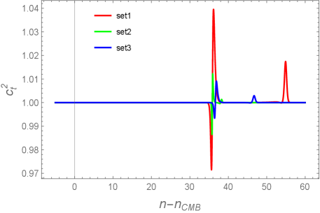
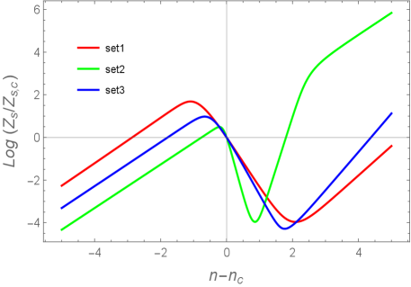
The scalar-GB coupling generally gives rise to the tensor and scalar propagation speeds different from 1. In the left panel of Fig. 3, we show the evolution of versus the number of e-foldings for the three sets of model parameters in Table 1. Just after the entry to the transient regime around , exhibits the deviation from 1. During the USR stage realized for the Set 1 model parameters, the field velocity is significantly suppressed and hence approaches 1. Just after the inflaton field exits from the USR regime, there is the temporal deviation of from 1. In the subsequent slow-roll regime, again goes back to 1. For the bump-type potential, which corresponds to the Set 2 model parameters, the time variation of occurs instantly in the vicinity of . In all the cases shown in the left panel of Fig. 3, the deviation of from 1 is insignificant () and hence the stability condition is always satisfied.
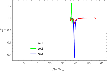
In the right panel of Fig. 3, we plot versus for the same sets of model parameters as those used in the left. For scalar perturbations, the no-ghost quantity is proportional to . Since appears in the denominator of in Eq. (14), a smaller does not imply a value of closer to 1. Indeed, during the transient regime around , the scalar propagation speeds deviate from 1 in all the three cases shown in Fig. 3. For Set 1, the minimum value of reached during the USR regime is about 0.91. The bump-type potential corresponds to the Set 2 model parameters, in which case temporally increases to the superluminal region and then quickly evolves to the minimum around . For Set 3, decreases to the minimum around 0.35 and returns back to the value close to 1 in the slow-roll regime. Since the positivity of holds in all these cases, there are no Laplacian instabilities for scalar perturbations.
Depending on the model parameters, there are cases in which the scalar sound speed enters the region . Since such models should be excluded by the Laplacian instability, we will focus on the case in subsequent sections.
IV.2 Primordial scalar power spectrum
To study the evolution of curvature perturbations during inflation, we introduce the “sound-horizon” time defined by
| (41) |
where . Then, the second-order action (13) of scalar perturbations reduces to
| (42) |
where a prime represents the derivative with respect to . We decompose the curvature perturbation into the Fourier modes as
| (43) |
where is a comoving wavenumber, and and are annihilation and creation operators, respectively. Introducing the rescaled field
| (44) |
we obtain the following differential equation
| (45) |
For the perturbations deep inside the sound-horizon (), is suppressed relative to . For such modes, we choose a positive-frequency solution in a Bunch-Davies vacuum state, i.e.,
| (46) |
as an initial condition. In practice, we set the initial time for each wavenumber that corresponds to 6 e-foldings before the sound-horizon crossing, i.e., at . Numerically we integrate Eq. (45) by the end of inflation (characterized by the time ) and compute the scalar power spectrum given by
| (47) |
We evaluate for three sets of model parameters given in Table 1. At the 60 e-foldings before the end of inflation, the observed amplitude on CMB scales is used to give a constraint among the model parameters. The two constants and in Table 1 are chosen to realize the sufficient enhancement of around .
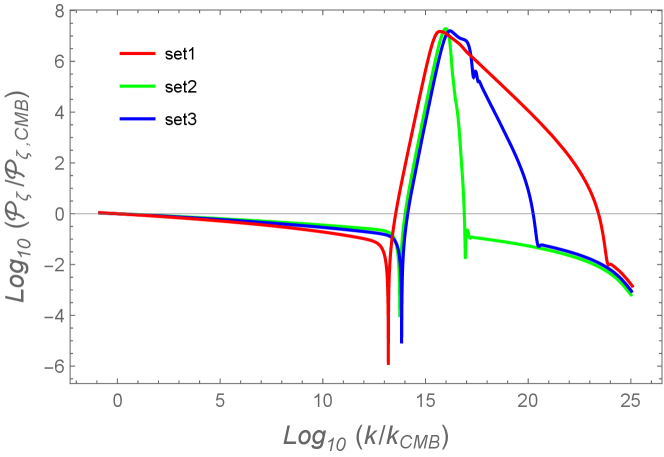
In Fig. 4, we show the primordial scalar power spectrum for three sets of model parameters. In comparison to the value of on the CMB scale (characterized by the comoving wavenumber of order Mpc), there is an enhancement of by a factor of . While the heights of peaks are similar between the three sets of parameters, the widths of are different from each other. The latter property is mostly attributed to the fact that the number of e-foldings acquired around are different between the plateau-, bump-, and intermediate-types.
Let us try to understand how the enhancement of around occurs in detail. For the perturbations outside the sound horizon (), Eq. (45) is approximately given by
| (48) |
The solution to this equation can be generally expressed in the form
| (49) |
where and are constants. On using the approximations and in the regimes and , the no-ghost parameter in Eq. (19) approximately reduces to
| (50) |
which is positive. Since we are considering the scalar-field evolution with , the quantity has the dependence
| (51) |
During the slow-roll regime in which the contribution from the scalar-GB coupling is negligible, the field derivative changes slowly with . In the limit that is constant, we have and hence the last term of Eq. (49) decays in proportion to on the quasi de-Sitter background (where ). Then, after the sound horizon crossing, approaches a constant value .
On the other hand, the field derivative exhibits a temporal rapid decrease during the transition around . Since the scalar-field solution in the USR regime arising from the plateau-type effective potential is given by , neglecting the time dependence of leads to the approximate relation . Then, the last term in Eq. (49) increases in proportion to . This means that the decaying mode in the slow-roll regime is replaced by the rapidly growing mode in the USR regime. Since also decreases rapidly for bump- and intermediate-type potentials, the curvature perturbation can be strongly enhanced around as well.
In the left panel of Fig. 5, we plot versus for three sets of model parameters in Table 1. During the initial slow-roll regime, the evolution of is approximately given by in all these three cases. For Set 1, which corresponds to the plateau-type potential, we find that decreases as in the vicinity of as expected. As we see in the right panel of Fig. 3, the deviation of from 1 is insignificant for Set 1 model parameters and hence the evolution of is hardly affected by the variation of .
The bump-type potential realized by Set 2 model parameters leads to a larger decreasing rate of around in comparison to the plateau-type because of the stronger suppression of (see the right panel of Fig. 2). For Set 2, the scalar sound speed temporally enters the region with a shorter transient period around in comparison to Set 1. For Set 3, which corresponds to the intermediate-type potential, the decreasing rate of is between those of the plateau- and bump-types. In all these cases, ’s begin to increase after reaching their minima, whose behavior is correlated with the evolution of plotted in Fig. 2.
In the superhorizon regime, the enhancement of depends on the integral of with respect to . On the other hand, we recall that we ignored the term in Eq. (45) relative to in the above argument. To understand which modes of are subject to the amplification, we explicitly compute as
| (52) |
where
| (53) |
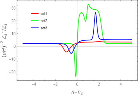
In the regime of slow-roll inflation, we have the approximate relation and hence soon approaches a constant after the Hubble radius crossing (). During the transient regime around , the quantities defined in Eq. (53) can be larger than order 1. In the right panel of Fig. 5, we plot versus for three sets of model parameters. For Set 1, starts to evolve from the value close to 2, temporally shows some decrease, and again increases to the value around 4. This means that, for the wavenumbers in the range , there is the enhancement of when the scalar field evolves along the plateau region of . For the perturbations which crossed the Hubble radius in the preceding slow-roll period, the last integral in Eq. (49) has already decayed sufficiently around the time at which approaches . Hence the enhanced modes of are those crossed the Hubble radius during the transient epoch around .
For Set 2, we observe in Fig. 5 that quickly reaches the value around 25 in the range . This means that curvature perturbations up to the wavenumber , which include subhorizon modes, can be amplified. In comparison to Set 1, the shorter transient period around still limits the range of for enhanced modes, see Fig. 4. Nevertheless, the height of peak of in Set 2 is similar to that in Set 1 thanks to the rapid increase of . For Set 3, the enhanced scalar power spectrum spans in the ranges of between those of Sets 1 and 2. In this case, the rapid decrease of seen in the right panel of Fig. 3 generates a sharp peak in . This gives rise to a shape of whose peak structure is different from those in other two cases. As we will see in Sec. V, the PBH abundance generated by these three sets of primordial power spectra can be sufficiently large to serve as almost all DM.
IV.3 CMB constraints
The existence of the transient regime with strongly suppressed values of modifies the spectra of scalar and tensor perturbations on scales relevant to the observed CMB temperature anisotropies. Besides Eq. (45), we also numerically solve the equation of tensor perturbations following from the second-order action (17). We then compute the CMB observables like , , and around the e-foldings backward from the end of inflation.
As we see in Fig. 2, the inflaton field stays nearly constant in the region around . In this transient regime, the acquired number of e-foldings is different depending on the model parameters. For larger , the field value around the CMB scale tends to be smaller. Since stays nearly constant during the transient regime, we can simply replace the relation (which was derived for in the limit ) with and . Then, it follows that
| (54) |
In the USR case corresponding to the Set 1 model parameters in Fig. 2, we have with and hence from Eq. (54). This shows good agreement with the numerical value of .
From Eqs. (25) and (26), the scalar power spectrum on CMB scales is known by the replacement , while the tensor power spectrum is hardly subject to modifications by the scalar-GB coupling. Applying the change to Eqs. (25), (27), and (28), we obtain
| (55) | |||||
| (56) | |||||
| (57) |
For larger , these observables exhibit more significant deviations from those in standard Higgs inflation. The values of in Table 1 are chosen to match the amplitude constrained by the Planck CMB data.
| \addstackgap [.5] | ||
|---|---|---|
| \addstackgap [.5] Set 1 | 0.951415 | 0.00757526 |
| \addstackgap [.5] Set 2 | 0.965142 | 0.00347235 |
| \addstackgap [.5] Set 3 | 0.960055 | 0.00476115 |
| \addstackgap [.5] Higgs inflation | 0.966527 | 0.00323724 |
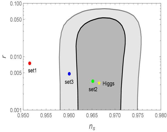
For the Set 1 model parameters in Table 1, substituting and into the analytic estimations of Eqs. (56) and (57) gives and . These are close to the numerically derived values presented in the first column of Table 2. In Fig. 6, we show the and observational bounds constrained from Planck 2018 data combined with the data of B-mode polarizations available from the BICEP2/Keck field (BK14) and baryon acoustic oscillations (BAO) Akrami et al. (2020). The theoretical values of and for Set 1 are outside the observational contour, so the plateau-type effective potential with is disfavored from the data. Unless we choose an unusually large value of exceeding 68, the model with does not enter the inside of the contour.
For Set 2, the number of e-foldings acquired around the bump region of is as small as , so the CMB observables are similar to those in standard Higgs inflation, see the second and fourth columns in Table 2. As we observe in Fig. 6, the model with Set 2 is inside the observational contour. For Set 3, we numerically obtain the values of and given in the third column of Table 2, with . In this case, the model is between and observational contours in the () plane. For , the number of e-foldings acquired around should be in the ranges
| (58) | |||
| (59) |
for the consistency with observations of and at and confidence levels, respectively. Thus, the bump-type model with a few is favored over the plateau-type model with from the viewpoint of CMB constraints.
On using the Planck normalized value in Eq. (55) together with Eq. (56), we obtain the following relations
| (60) |
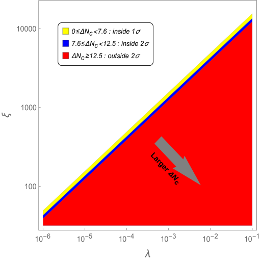
Fixing to be 60, the scalar spectral index is in the range for . This means that, from Eq. (60), the ratio is in the range . As increases, gets larger. The and confidence regions of , which are given by Eqs. (58) and (59) respectively, translate to
| (61) | |||
| (62) |
In Fig. 7, these parameter spaces are plotted as yellow () and blue () regions in the plane. The red region is outside the observational contour. The allowed parameter spaces shown in Fig. 7 will be useful to put further constraints on the values of and from future collider experiments.
V PBH abundance
After inflation the perturbations reenter the Hubble radius, whose epoch depends on the comoving wavenumber . In Sec. IV, we showed that the presence of the scalar-GB coupling can lead to the sufficient amplification of curvature perturbations during inflation for particular wavelengths smaller than the CMB scale ( Mpc). Such overdense regions can collapse to form PBHs after the horizon reentry.
The horizon mass associated with the Hubble distance is given by . The mass of PBHs at its formation time can be expressed as Green et al. (2004)
| (63) |
where is the ratio of how much of the inner region of the Hubble radius collapses into PBHs. We will consider the case in which the formation of PBHs occurs during the radiation-dominated epoch. The Hubble parameter at is related to today’s Hubble constant as Kawai and Kim (2021a)
| (64) |
where the subscript “0” represents today’s values and is the relativistic degrees of freedom. The wavenumber at horizon reentry corresponds to , whose relation can be used to eliminate in Eq. (64). Solving Eq. (64) for and substituting it into Eq. (63), it follows that
| (65) |
where we used the values , , and GeV.
The abundance of PBHs can be estimated by using the Press-Schechter theory. Assuming a Gaussian distribution for the coarse-grained density fluctuation , the probability that is higher than a certain threshold value at is given by Green et al. (2004); Young et al. (2014); Harada et al. (2013); Germani and Musco (2019)
| (66) |
where
| (67) |
The window function determines how the density contrast around is coarse-grained, where is the density and is its background part. We choose the Gaussian window function of the form
| (68) |
where the distance is taken to be . Then, the variance of is given by
| (69) |
Since the PBH density decreases as after its formation, today’s PBH density can be estimated as
| (70) |
Since is related to as , today’s density parameter of PBHs corresponding to Eq. (70) is
| (71) |
with total PBH density parameter . Then, we obtain the ratio of the PBH abundance in a mass range to the entire density of cold DM (today’s density parameter ) as
| (72) |
where km sec-1 Mpc-1.
In the following, we use the values Carr (1975), , , and for the computations of and . With a given wavenumber at horizon reentry, the PBH mass is known from Eq. (65). The variance (69) is affected by the primordial spectrum enhanced at some particular scales during inflation. This modifies the PBH mass function through the change of in Eq. (66).
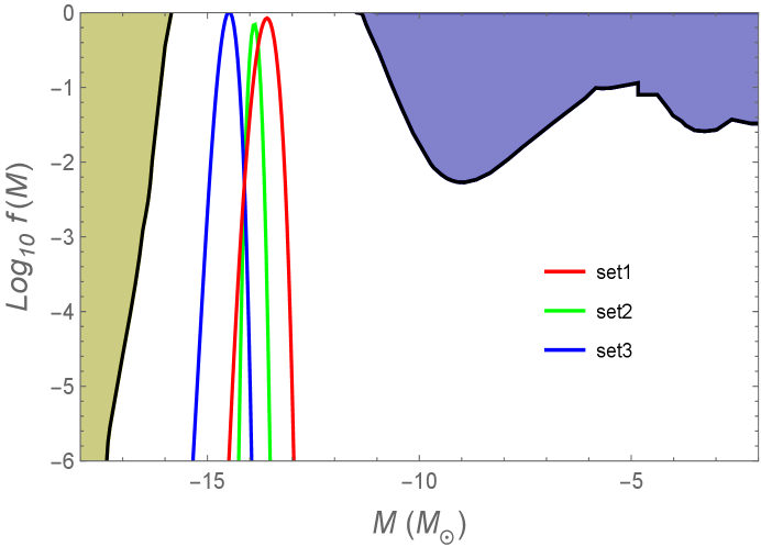
In Fig. 8, we plot versus for the three sets of model parameters presented in Table 1. In these three cases, the mass functions span in the range . As we observe in Fig. 4, the wavenumber corresponding to the peak positions of is smallest for Set 1, while largest for Set 3. From Eq. (65), the PBH mass decreases for larger . Then, the mass corresponding to the peaks of is smallest for Set 3, while largest for Set 1. The maximum values of are found to be , , and for Sets 1, 2, 3, respectively, so PBHs are the source for practically all cold DM in these three cases.
In Fig. 8, we also show the regions excluded by the black hole evaporation and by microlensing observations. The models with Sets 1, 2, 3 are also consistent with such constraints. While we have considered the PBH mass range , it is also possible to produce PBHs with the mass by choosing different sets of model parameters. The heights of peaks of can be also lower than the order 0.1 to be consistent with the microlensing data. Thus, our model allows versatile possibilities for generating PBHs in broad mass ranges.
Finally, we explicitly derive a relation between and the critical field value . This is useful for estimating the mass of PBH and determining the model parameters. After the transient regime the inflationary dynamics rapidly approaches the slow-roll solution, so we can exploit Eq. (23) as a good approximation. Then, we obtain
| (73) |
where and represent the moments at which the CMB and PBH scales leave the Hubble horizon, respectively. From Eq. (65), we can estimate as
| (74) |
where we used the values , , and in the last equality. Substituting Eq. (74) into Eq. (73), it follows that
| (75) |
In the USR case corresponding to Set 1 model parameters, for example, we have and , and hence from Eq. (75). This is in good agreement with the exact value of , i.e., . For the PBH mass range in which PBHs can be the source for all DM, the corresponding region of is given by
| (76) |
We recall that, for the plateau-type potential, and are related to according to Eqs. (36) and (37), respectively. By using these relations with Eq. (75), the orders of parameters and are known for given values of and . We caution that the relations (36) and (37) lose their accuracy for the bump-type potential, but they are still useful to estimate the orders of and . To know the precise values of and with which curvature perturbations are sufficiently enhanced for scales relevant to PBHs, the numerical analysis is required as we performed in Sec. IV. Basically, and determine the height of enhancement of and the length of transient period, respectively.
VI Conclusions
We studied a mechanism for producing the seed of PBHs in Higgs inflation in the presence of a scalar-GB coupling. This provides a minimal scenario of inflation within a framework of standard model of particle physics, while allowing for the compatibility with observed CMB temperature anisotropies. In comparison to original Higgs inflation, however, the scalar-GB coupling can modify theoretical predictions of the scalar spectral index and tensor-to-scalar ratio on CMB scales. We explored the possibility for enhancing curvature perturbations at some particular scales to generate the seed for PBHs, while the model is still compatible with the CMB observations.
The enhancement of curvature perturbations during inflation is possible when the inflaton velocity rapidly decreases toward 0 during some transient epoch. If there is a period in which the scalar-GB coupling quickly changes, it is possible to generate particular shapes in the inflaton effective potential . For this purpose, we considered a coupling function of the form , where is the field value at transition. Since approaches constants in two asymptotic regimes and , the scalar-GB coupling affects the dynamics of background and perturbations only in the vicinity of . Depending on the model parameters, the effective potential can be classified into three classes: (1) plateau-type, (2) bump-type, (3) intermediate-type.
A typical example of the plateau-type is the Set 1 model parameters given in Table 1, in which case the scalar-GB coupling almost balances the potential and nonminimal coupling terms around . For this type the effective potential has a nearly flat region, as seen in the left panel of Fig. 1. During the USR regime, the field derivative decreases as . As we observe in the left panel of Fig. 2 for Set 1, the number of e-foldings acquired around is as large as 20. The Set 2 model parameters in Table 1 give rise to a bump-type potential illustrated in the middle panel of Fig. 1. In this case, the existence of an explicit peak in leads to the approach of toward 0 even faster than the USR case. For Set 2, the number of e-foldings acquired around is as small as a few. The Set 3 model parameters in Table 1 correspond to the intermediate-type potential plotted in the right panel of Fig. 1. For this type, both the decreasing rate of and are between those of plateau- and bump-types.
The evolution of scalar perturbations during inflation crucially depends on the quantity defined in Eq. (44). After the sound horizon crossing, the solution to the Fourier-transformed curvature perturbation is expressed in the form (49). In all the three types of mentioned above, rapidly decreases in the vicinity of . Since the last integral in Eq. (49) becomes a rapidly growing mode during the transient regime, there is the strong enhancement of for the modes exiting the sound horizon around . For the effective potential closer to the bump-type, the quantity , which appears in the equation of motion for , can exceed the order of during the rapid transition. Then, the bump-type potential also leads to the amplification of some subhorizon modes. Still, the shapes of primordial scalar power spectra mostly depend on the number of e-foldings , in such a way that the peak tends to be sharper for smaller .
The primordial power spectra plotted in Fig. 4 correspond to those of Set 1, 2, 3 model parameters. In all these cases, the peak values of are about times as large as the amplitude of on CMB scales. With these model parameters, all the stability conditions given in Eq. (18) are consistently satisfied and hence there are neither ghost nor Laplacian instabilities. We note that the inflaton-GB coupling gives rise to the scalar propagation speed different from 1, whose property also affects the shapes of .
The existence of the transient epoch around modifies the scalar power spectrum and tensor-to-scalar ratio on CMB scales. In standard Higgs inflation, the expressions of , , and are given, respectively, by Eqs. (25), (27), and (28), where is the number of e-foldings counted backward from the end of inflation. In the presence of the scalar-GB coupling, these observables are subject to the modification , where corresponds to the number of e-foldings on CMB scales. This means that, for smaller , the models can exhibit better compatibility with the observational bounds on and . As we see in Fig. 6, the bump-type with (Set 2) is well inside the observational contour constrained from CMB and other data, while the plateau-type with (Set 1) is outside the contour. The intermediate-type model with (Set 3) is between and contours. These results show that the bump-type is generally favored over the plateau-type from the CMB constraints.
In Fig. 8, we plot the PBH fraction function versus the mass for three sets of model parameters in Table 1. In all these cases we have in the mass range . Thus, the GB corrected Higgs inflation allows the possibility for generating the amount of PBHs serving as almost all DM, while being compatible with the observed temperature anisotropies on CMB scales especially for the bump-type effective potential. We note that, in our model, it is also possible to generate PBHs in the larger mass range with the fraction .
The enhanced primordial curvature perturbations on particular scales may induce gravitational waves at nonlinear order, which affects the spectrum of gravitational wave background Kohri and Terada (2018) (see also Ref. Papanikolaou et al. (2021)). In addition, while a Gaussian distribution was used for the coarse-grained density fluctuation in this paper, it was reported that the distribution function of curvature fluctuations may have a peculiar shape deviating from the Gaussian Namjoo et al. (2013); Franciolini et al. (2018); Cai et al. (2018b); Atal and Germani (2019); Atal et al. (2019, 2020); Passaglia et al. (2019); Taoso and Urbano (2021); Biagetti et al. (2021); Davies et al. (2022); Cai et al. (2022a, b). Recently, it was shown that the PBH scenario in single-field inflation with an USR regime can induce large one-loop corrections to the scalar power spectrum on CMB scales Kristiano and Yokoyama (2022); Inomata et al. (2022b). Since the analysis is limited to a canonical scalar field with a plateau-type potential, the results of Ref. Kristiano and Yokoyama (2022) are not applied to our model in which the enhancement of curvature perturbations occurs by the presence of the inflaton-GB coupling. However, it is worth computing one-loop corrections to in our model, especially for the bump-type effective potential. We leave these interesting issues for future works.
Acknowledgments
We thank Tomohiro Fujita for useful discussions and comments. We also thank Bradley Kavanagh for giving us permission to use observational constraints given in Fig. 8. ST is supported by the Grant-in-Aid for Scientific Research Fund of the JSPS Nos. 19K03854 and 22K03642.
Appendix A Appendix: Correspondence with Horndeski theory
The inflationary model studied in this paper belongs to a subclass of Horndeski theory given by the action Horndeski (1974); Deffayet et al. (2011); Kobayashi et al. (2011); Charmousis et al. (2012)
| (77) |
where
| (78) | |||||
with being the Einstein tensor. Four functions ’s () depend on the scalar field and its kinetic term , where we use the notation . The action (1) can be accommodated by the following coupling functions Kobayashi et al. (2011)
| (79) | |||
| (80) | |||
| (81) | |||
| (82) |
where . In full Horndeski theories, the background and perturbation equations of motion on the flat FLRW background were already derived in Refs. Kobayashi et al. (2011); De Felice and Tsujikawa (2011b); De Felice et al. (2011). In this paper, we applied those results to the theory given by the coupling functions (79)-(82).
References
- Zel’dovich and Novikov (1967) Y. B. Zel’dovich and I. D. Novikov, Soviet Astronomy 10, 602 (1967).
- Hawking (1971) S. Hawking, Mon. Not. Roy. Astron. Soc. 152, 75 (1971).
- Carr and Hawking (1974) B. J. Carr and S. W. Hawking, Mon. Not. Roy. Astron. Soc. 168, 399 (1974).
- Chapline (1975) G. F. Chapline, Nature 253, 251 (1975).
- Meszaros (1975) P. Meszaros, Astron. Astrophys. 38, 5 (1975).
- Khlopov (2010) M. Y. Khlopov, Res. Astron. Astrophys. 10, 495 (2010), arXiv:0801.0116 [astro-ph] .
- Sasaki et al. (2018) M. Sasaki, T. Suyama, T. Tanaka, and S. Yokoyama, Class. Quant. Grav. 35, 063001 (2018), arXiv:1801.05235 [astro-ph.CO] .
- Carr and Kuhnel (2020) B. Carr and F. Kuhnel, Ann. Rev. Nucl. Part. Sci. 70, 355 (2020), arXiv:2006.02838 [astro-ph.CO] .
- Green and Kavanagh (2021) A. M. Green and B. J. Kavanagh, J. Phys. G 48, 043001 (2021), arXiv:2007.10722 [astro-ph.CO] .
- Villanueva-Domingo et al. (2021) P. Villanueva-Domingo, O. Mena, and S. Palomares-Ruiz, Front. Astron. Space Sci. 8, 87 (2021), arXiv:2103.12087 [astro-ph.CO] .
- Carr and Kuhnel (2022) B. Carr and F. Kuhnel, SciPost Phys. Lect. Notes 48, 1 (2022), arXiv:2110.02821 [astro-ph.CO] .
- Escrivà et al. (2022) A. Escrivà, F. Kuhnel, and Y. Tada, arXiv:2211.05767 [astro-ph.CO] .
- Karam et al. (2022) A. Karam, N. Koivunen, E. Tomberg, V. Vaskonen, and H. Veermäe, arXiv:2205.13540 [astro-ph.CO] .
- Abbott et al. (2016) B. P. Abbott et al. (LIGO Scientific, Virgo), Phys. Rev. Lett. 116, 061102 (2016), arXiv:1602.03837 [gr-qc] .
- Abbott et al. (2019) B. P. Abbott et al. (LIGO Scientific, Virgo), Phys. Rev. X 9, 031040 (2019), arXiv:1811.12907 [astro-ph.HE] .
- Abbott et al. (2021a) R. Abbott et al. (LIGO Scientific, Virgo), Phys. Rev. X 11, 021053 (2021a), arXiv:2010.14527 [gr-qc] .
- Abbott et al. (2021b) R. Abbott et al. (LIGO Scientific, VIRGO, KAGRA), arXiv:2111.03606 [gr-qc] .
- Bird et al. (2016) S. Bird, I. Cholis, J. B. Muñoz, Y. Ali-Haïmoud, M. Kamionkowski, E. D. Kovetz, A. Raccanelli, and A. G. Riess, Phys. Rev. Lett. 116, 201301 (2016), arXiv:1603.00464 [astro-ph.CO] .
- Sasaki et al. (2016) M. Sasaki, T. Suyama, T. Tanaka, and S. Yokoyama, Phys. Rev. Lett. 117, 061101 (2016), [Erratum: Phys.Rev.Lett. 121, 059901 (2018)], arXiv:1603.08338 [astro-ph.CO] .
- Clesse and García-Bellido (2017) S. Clesse and J. García-Bellido, Phys. Dark Univ. 15, 142 (2017), arXiv:1603.05234 [astro-ph.CO] .
- Wang et al. (2018) S. Wang, Y.-F. Wang, Q.-G. Huang, and T. G. F. Li, Phys. Rev. Lett. 120, 191102 (2018), arXiv:1610.08725 [astro-ph.CO] .
- Bean and Magueijo (2002) R. Bean and J. Magueijo, Phys. Rev. D 66, 063505 (2002), arXiv:astro-ph/0204486 .
- Carr et al. (2021) B. Carr, K. Kohri, Y. Sendouda, and J. Yokoyama, Rept. Prog. Phys. 84, 116902 (2021), arXiv:2002.12778 [astro-ph.CO] .
- Ivanov et al. (1994) P. Ivanov, P. Naselsky, and I. Novikov, Phys. Rev. D 50, 7173 (1994).
- Garcia-Bellido et al. (1996) J. Garcia-Bellido, A. D. Linde, and D. Wands, Phys. Rev. D 54, 6040 (1996), arXiv:astro-ph/9605094 .
- Bullock and Primack (1997) J. S. Bullock and J. R. Primack, Phys. Rev. D 55, 7423 (1997), arXiv:astro-ph/9611106 .
- Yokoyama (1997) J. Yokoyama, Astron. Astrophys. 318, 673 (1997), arXiv:astro-ph/9509027 .
- Yokoyama (1998) J. Yokoyama, Phys. Rev. D 58, 083510 (1998), arXiv:astro-ph/9802357 .
- Kawasaki et al. (1998) M. Kawasaki, N. Sugiyama, and T. Yanagida, Phys. Rev. D 57, 6050 (1998), arXiv:hep-ph/9710259 .
- Kawasaki et al. (2006) M. Kawasaki, T. Takayama, M. Yamaguchi, and J. Yokoyama, Phys. Rev. D 74, 043525 (2006), arXiv:hep-ph/0605271 .
- Kohri et al. (2008) K. Kohri, D. H. Lyth, and A. Melchiorri, JCAP 04, 038 (2008), arXiv:0711.5006 [hep-ph] .
- Saito et al. (2008) R. Saito, J. Yokoyama, and R. Nagata, JCAP 06, 024 (2008), arXiv:0804.3470 [astro-ph] .
- Bugaev and Klimai (2008) E. Bugaev and P. Klimai, Phys. Rev. D 78, 063515 (2008), arXiv:0806.4541 [astro-ph] .
- Alabidi and Kohri (2009) L. Alabidi and K. Kohri, Phys. Rev. D 80, 063511 (2009), arXiv:0906.1398 [astro-ph.CO] .
- Drees and Erfani (2011) M. Drees and E. Erfani, JCAP 04, 005 (2011), arXiv:1102.2340 [hep-ph] .
- Drees and Erfani (2012) M. Drees and E. Erfani, JCAP 01, 035 (2012), arXiv:1110.6052 [astro-ph.CO] .
- Martin et al. (2013) J. Martin, H. Motohashi, and T. Suyama, Phys. Rev. D 87, 023514 (2013), arXiv:1211.0083 [astro-ph.CO] .
- Kohri et al. (2013) K. Kohri, C.-M. Lin, and T. Matsuda, Phys. Rev. D 87, 103527 (2013), arXiv:1211.2371 [hep-ph] .
- Kawasaki et al. (2013) M. Kawasaki, N. Kitajima, and T. T. Yanagida, Phys. Rev. D 87, 063519 (2013), arXiv:1207.2550 [hep-ph] .
- Clesse and García-Bellido (2015) S. Clesse and J. García-Bellido, Phys. Rev. D 92, 023524 (2015), arXiv:1501.07565 [astro-ph.CO] .
- Kawasaki and Tada (2016) M. Kawasaki and Y. Tada, JCAP 08, 041 (2016), arXiv:1512.03515 [astro-ph.CO] .
- Kawasaki et al. (2016) M. Kawasaki, A. Kusenko, Y. Tada, and T. T. Yanagida, Phys. Rev. D 94, 083523 (2016), arXiv:1606.07631 [astro-ph.CO] .
- Pi et al. (2018) S. Pi, Y.-l. Zhang, Q.-G. Huang, and M. Sasaki, JCAP 05, 042 (2018), arXiv:1712.09896 [astro-ph.CO] .
- Garcia-Bellido and Ruiz Morales (2017) J. Garcia-Bellido and E. Ruiz Morales, Phys. Dark Univ. 18, 47 (2017), arXiv:1702.03901 [astro-ph.CO] .
- Kannike et al. (2017) K. Kannike, L. Marzola, M. Raidal, and H. Veermäe, JCAP 09, 020 (2017), arXiv:1705.06225 [astro-ph.CO] .
- Germani and Prokopec (2017) C. Germani and T. Prokopec, Phys. Dark Univ. 18, 6 (2017), arXiv:1706.04226 [astro-ph.CO] .
- Ando et al. (2018) K. Ando, K. Inomata, M. Kawasaki, K. Mukaida, and T. T. Yanagida, Phys. Rev. D 97, 123512 (2018), arXiv:1711.08956 [astro-ph.CO] .
- Ezquiaga et al. (2018) J. M. Ezquiaga, J. Garcia-Bellido, and E. Ruiz Morales, Phys. Lett. B 776, 345 (2018), arXiv:1705.04861 [astro-ph.CO] .
- Motohashi and Hu (2017) H. Motohashi and W. Hu, Phys. Rev. D 96, 063503 (2017), arXiv:1706.06784 [astro-ph.CO] .
- Di and Gong (2018) H. Di and Y. Gong, JCAP 07, 007 (2018), arXiv:1707.09578 [astro-ph.CO] .
- Ballesteros and Taoso (2018) G. Ballesteros and M. Taoso, Phys. Rev. D 97, 023501 (2018), arXiv:1709.05565 [hep-ph] .
- Garcia-Bellido et al. (2017) J. Garcia-Bellido, M. Peloso, and C. Unal, JCAP 09, 013 (2017), arXiv:1707.02441 [astro-ph.CO] .
- Hertzberg and Yamada (2018) M. P. Hertzberg and M. Yamada, Phys. Rev. D 97, 083509 (2018), arXiv:1712.09750 [astro-ph.CO] .
- Inomata et al. (2018) K. Inomata, M. Kawasaki, K. Mukaida, and T. T. Yanagida, Phys. Rev. D 97, 043514 (2018), arXiv:1711.06129 [astro-ph.CO] .
- Cai et al. (2018a) Y.-F. Cai, X. Tong, D.-G. Wang, and S.-F. Yan, Phys. Rev. Lett. 121, 081306 (2018a), arXiv:1805.03639 [astro-ph.CO] .
- Drees and Xu (2021) M. Drees and Y. Xu, Eur. Phys. J. C 81, 182 (2021), arXiv:1905.13581 [hep-ph] .
- Atal et al. (2019) V. Atal, J. Garriga, and A. Marcos-Caballero, JCAP 09, 073 (2019), arXiv:1905.13202 [astro-ph.CO] .
- Atal et al. (2020) V. Atal, J. Cid, A. Escrivà, and J. Garriga, JCAP 05, 022 (2020), arXiv:1908.11357 [astro-ph.CO] .
- Mishra and Sahni (2020) S. S. Mishra and V. Sahni, JCAP 04, 007 (2020), arXiv:1911.00057 [gr-qc] .
- Cheong et al. (2021) D. Y. Cheong, S. M. Lee, and S. C. Park, JCAP 01, 032 (2021), arXiv:1912.12032 [hep-ph] .
- Fu et al. (2019) C. Fu, P. Wu, and H. Yu, Phys. Rev. D 100, 063532 (2019), arXiv:1907.05042 [astro-ph.CO] .
- Dalianis et al. (2020) I. Dalianis, S. Karydas, and E. Papantonopoulos, JCAP 06, 040 (2020), arXiv:1910.00622 [astro-ph.CO] .
- Ashoorioon et al. (2021) A. Ashoorioon, A. Rostami, and J. T. Firouzjaee, JHEP 07, 087 (2021), arXiv:1912.13326 [astro-ph.CO] .
- Lin et al. (2020) J. Lin, Q. Gao, Y. Gong, Y. Lu, C. Zhang, and F. Zhang, Phys. Rev. D 101, 103515 (2020), arXiv:2001.05909 [gr-qc] .
- Yi et al. (2021) Z. Yi, Y. Gong, B. Wang, and Z.-h. Zhu, Phys. Rev. D 103, 063535 (2021), arXiv:2007.09957 [gr-qc] .
- Palma et al. (2020) G. A. Palma, S. Sypsas, and C. Zenteno, Phys. Rev. Lett. 125, 121301 (2020), arXiv:2004.06106 [astro-ph.CO] .
- Braglia et al. (2020) M. Braglia, D. K. Hazra, F. Finelli, G. F. Smoot, L. Sriramkumar, and A. A. Starobinsky, JCAP 08, 001 (2020), arXiv:2005.02895 [astro-ph.CO] .
- Kefala et al. (2021) K. Kefala, G. P. Kodaxis, I. D. Stamou, and N. Tetradis, Phys. Rev. D 104, 023506 (2021), arXiv:2010.12483 [astro-ph.CO] .
- Ballesteros et al. (2020) G. Ballesteros, J. Rey, M. Taoso, and A. Urbano, JCAP 07, 025 (2020), arXiv:2001.08220 [astro-ph.CO] .
- Aldabergenov et al. (2020) Y. Aldabergenov, A. Addazi, and S. V. Ketov, Eur. Phys. J. C 80, 917 (2020), arXiv:2006.16641 [hep-th] .
- Aldabergenov et al. (2021) Y. Aldabergenov, A. Addazi, and S. V. Ketov, Phys. Lett. B 814, 136069 (2021), arXiv:2008.10476 [hep-th] .
- Inomata et al. (2021) K. Inomata, E. McDonough, and W. Hu, Phys. Rev. D 104, 123553 (2021), arXiv:2104.03972 [astro-ph.CO] .
- Inomata et al. (2022a) K. Inomata, E. McDonough, and W. Hu, JCAP 02, 031 (2022a), arXiv:2110.14641 [astro-ph.CO] .
- Dalianis et al. (2021) I. Dalianis, G. P. Kodaxis, I. D. Stamou, N. Tetradis, and A. Tsigkas-Kouvelis, Phys. Rev. D 104, 103510 (2021), arXiv:2106.02467 [astro-ph.CO] .
- Cai et al. (2022a) Y.-F. Cai, X.-H. Ma, M. Sasaki, D.-G. Wang, and Z. Zhou, Phys. Lett. B 834, 137461 (2022a), arXiv:2112.13836 [astro-ph.CO] .
- Lin et al. (2021) J. Lin, S. Gao, Y. Gong, Y. Lu, Z. Wang, and F. Zhang, arXiv:2111.01362 [gr-qc] .
- Kawai and Kim (2021a) S. Kawai and J. Kim, Phys. Rev. D 104, 083545 (2021a), arXiv:2108.01340 [astro-ph.CO] .
- Zhang (2022) F. Zhang, Phys. Rev. D 105, 063539 (2022), arXiv:2112.10516 [gr-qc] .
- Ahmed et al. (2022) W. Ahmed, M. Junaid, and U. Zubair, Nucl. Phys. B 984, 115968 (2022), arXiv:2109.14838 [astro-ph.CO] .
- Cai et al. (2022b) Y.-F. Cai, X.-H. Ma, M. Sasaki, D.-G. Wang, and Z. Zhou, arXiv:2207.11910 [astro-ph.CO] .
- Pi and Wang (2022) S. Pi and J. Wang, arXiv:2209.14183 [astro-ph.CO] .
- Cheong et al. (2022) D. Y. Cheong, K. Kohri, and S. C. Park, JCAP 10, 015 (2022), arXiv:2205.14813 [hep-ph] .
- Kawai and Kim (2022) S. Kawai and J. Kim, arXiv:2209.15343 [astro-ph.CO] .
- Akrami et al. (2020) Y. Akrami et al. (Planck), Astron. Astrophys. 641, A10 (2020), arXiv:1807.06211 [astro-ph.CO] .
- Green and Malik (2001) A. M. Green and K. A. Malik, Phys. Rev. D 64, 021301 (2001), arXiv:hep-ph/0008113 .
- Bassett and Tsujikawa (2001) B. A. Bassett and S. Tsujikawa, Phys. Rev. D 63, 123503 (2001), arXiv:hep-ph/0008328 .
- Suyama et al. (2005) T. Suyama, T. Tanaka, B. Bassett, and H. Kudoh, Phys. Rev. D 71, 063507 (2005), arXiv:hep-ph/0410247 .
- Martin et al. (2020) J. Martin, T. Papanikolaou, and V. Vennin, JCAP 01, 024 (2020), arXiv:1907.04236 [astro-ph.CO] .
- Bezrukov and Shaposhnikov (2008) F. L. Bezrukov and M. Shaposhnikov, Phys. Lett. B 659, 703 (2008), arXiv:0710.3755 [hep-th] .
- Bezrukov et al. (2009) F. L. Bezrukov, A. Magnin, and M. Shaposhnikov, Phys. Lett. B 675, 88 (2009), arXiv:0812.4950 [hep-ph] .
- Bezrukov et al. (2011) F. Bezrukov, A. Magnin, M. Shaposhnikov, and S. Sibiryakov, JHEP 01, 016 (2011), arXiv:1008.5157 [hep-ph] .
- Futamase and Maeda (1989) T. Futamase and K.-i. Maeda, Phys. Rev. D 39, 399 (1989).
- Fakir and Unruh (1990) R. Fakir and W. G. Unruh, Phys. Rev. D 41, 1783 (1990).
- Komatsu and Futamase (1999) E. Komatsu and T. Futamase, Phys. Rev. D 59, 064029 (1999), arXiv:astro-ph/9901127 .
- Tsujikawa and Gumjudpai (2004) S. Tsujikawa and B. Gumjudpai, Phys. Rev. D 69, 123523 (2004), arXiv:astro-ph/0402185 .
- Linde et al. (2011) A. Linde, M. Noorbala, and A. Westphal, JCAP 03, 013 (2011), arXiv:1101.2652 [hep-th] .
- Ade et al. (2014) P. A. R. Ade et al. (Planck), Astron. Astrophys. 571, A22 (2014), arXiv:1303.5082 [astro-ph.CO] .
- Tsujikawa et al. (2013) S. Tsujikawa, J. Ohashi, S. Kuroyanagi, and A. De Felice, Phys. Rev. D 88, 023529 (2013), arXiv:1305.3044 [astro-ph.CO] .
- Hwang and Noh (2005) J.-c. Hwang and H. Noh, Phys. Rev. D 71, 063536 (2005), arXiv:gr-qc/0412126 .
- Guo et al. (2007) Z.-K. Guo, N. Ohta, and S. Tsujikawa, Phys. Rev. D 75, 023520 (2007), arXiv:hep-th/0610336 .
- Satoh and Soda (2008) M. Satoh and J. Soda, JCAP 09, 019 (2008), arXiv:0806.4594 [astro-ph] .
- Guo and Schwarz (2009) Z.-K. Guo and D. J. Schwarz, Phys. Rev. D 80, 063523 (2009), arXiv:0907.0427 [hep-th] .
- Guo and Schwarz (2010) Z.-K. Guo and D. J. Schwarz, Phys. Rev. D 81, 123520 (2010), arXiv:1001.1897 [hep-th] .
- Kawai and Kim (2021b) S. Kawai and J. Kim, Phys. Rev. D 104, 043525 (2021b), arXiv:2105.04386 [hep-ph] .
- Kobayashi et al. (2011) T. Kobayashi, M. Yamaguchi, and J. Yokoyama, Prog. Theor. Phys. 126, 511 (2011), arXiv:1105.5723 [hep-th] .
- Kase and Tsujikawa (2019) R. Kase and S. Tsujikawa, Int. J. Mod. Phys. D 28, 1942005 (2019), arXiv:1809.08735 [gr-qc] .
- Salopek et al. (1989) D. S. Salopek, J. R. Bond, and J. M. Bardeen, Phys. Rev. D 40, 1753 (1989).
- Makino and Sasaki (1991) N. Makino and M. Sasaki, Prog. Theor. Phys. 86, 103 (1991).
- Kaiser (1995) D. I. Kaiser, Phys. Rev. D 52, 4295 (1995), arXiv:astro-ph/9408044 .
- De Simone et al. (2009) A. De Simone, M. P. Hertzberg, and F. Wilczek, Phys. Lett. B 678, 1 (2009), arXiv:0812.4946 [hep-ph] .
- Hamada et al. (2014) Y. Hamada, H. Kawai, K.-y. Oda, and S. C. Park, Phys. Rev. Lett. 112, 241301 (2014), arXiv:1403.5043 [hep-ph] .
- Hamada et al. (2015) Y. Hamada, H. Kawai, K.-y. Oda, and S. C. Park, Phys. Rev. D 91, 053008 (2015), arXiv:1408.4864 [hep-ph] .
- Bezrukov et al. (2015) F. Bezrukov, J. Rubio, and M. Shaposhnikov, Phys. Rev. D 92, 083512 (2015), arXiv:1412.3811 [hep-ph] .
- Bezrukov et al. (2018) F. Bezrukov, M. Pauly, and J. Rubio, JCAP 02, 040 (2018), arXiv:1706.05007 [hep-ph] .
- Horndeski (1974) G. W. Horndeski, Int. J. Theor. Phys. 10, 363 (1974).
- Deffayet et al. (2011) C. Deffayet, X. Gao, D. A. Steer, and G. Zahariade, Phys. Rev. D 84, 064039 (2011), arXiv:1103.3260 [hep-th] .
- Charmousis et al. (2012) C. Charmousis, E. J. Copeland, A. Padilla, and P. M. Saffin, Phys. Rev. Lett. 108, 051101 (2012), arXiv:1106.2000 [hep-th] .
- De Felice and Tsujikawa (2011a) A. De Felice and S. Tsujikawa, JCAP 04, 029 (2011a), arXiv:1103.1172 [astro-ph.CO] .
- Gross and Sloan (1987) D. J. Gross and J. H. Sloan, Nucl. Phys. B 291, 41 (1987).
- Metsaev and Tseytlin (1987) R. R. Metsaev and A. A. Tseytlin, Nucl. Phys. B 293, 385 (1987).
- Gasperini et al. (1997) M. Gasperini, M. Maggiore, and G. Veneziano, Nucl. Phys. B 494, 315 (1997), arXiv:hep-th/9611039 .
- Kawai et al. (1998) S. Kawai, M.-a. Sakagami, and J. Soda, Phys. Lett. B 437, 284 (1998), arXiv:gr-qc/9802033 .
- Cartier et al. (2001) C. Cartier, J.-c. Hwang, and E. J. Copeland, Phys. Rev. D 64, 103504 (2001), arXiv:astro-ph/0106197 .
- Calcagni et al. (2005) G. Calcagni, S. Tsujikawa, and M. Sami, Class. Quant. Grav. 22, 3977 (2005), arXiv:hep-th/0505193 .
- Khan and Yogesh (2022) H. A. Khan and Yogesh, Phys. Rev. D 105, 063526 (2022), arXiv:2201.06439 [astro-ph.CO] .
- Green et al. (2004) A. M. Green, A. R. Liddle, K. A. Malik, and M. Sasaki, Phys. Rev. D 70, 041502 (2004), arXiv:astro-ph/0403181 .
- Young et al. (2014) S. Young, C. T. Byrnes, and M. Sasaki, JCAP 07, 045 (2014), arXiv:1405.7023 [gr-qc] .
- Harada et al. (2013) T. Harada, C.-M. Yoo, and K. Kohri, Phys. Rev. D 88, 084051 (2013), [Erratum: Phys.Rev.D 89, 029903 (2014)], arXiv:1309.4201 [astro-ph.CO] .
- Germani and Musco (2019) C. Germani and I. Musco, Phys. Rev. Lett. 122, 141302 (2019), arXiv:1805.04087 [astro-ph.CO] .
- Kavanagh (2019) B. J. Kavanagh, “bradkav/pbhbounds: Release version,” (2019).
- Carr (1975) B. J. Carr, Astrophys. J. 201, 1 (1975).
- Kohri and Terada (2018) K. Kohri and T. Terada, Phys. Rev. D 97, 123532 (2018), arXiv:1804.08577 [gr-qc] .
- Papanikolaou et al. (2021) T. Papanikolaou, V. Vennin, and D. Langlois, JCAP 03, 053 (2021), arXiv:2010.11573 [astro-ph.CO] .
- Namjoo et al. (2013) M. H. Namjoo, H. Firouzjahi, and M. Sasaki, EPL 101, 39001 (2013), arXiv:1210.3692 [astro-ph.CO] .
- Franciolini et al. (2018) G. Franciolini, A. Kehagias, S. Matarrese, and A. Riotto, JCAP 03, 016 (2018), arXiv:1801.09415 [astro-ph.CO] .
- Cai et al. (2018b) Y.-F. Cai, X. Chen, M. H. Namjoo, M. Sasaki, D.-G. Wang, and Z. Wang, JCAP 05, 012 (2018b), arXiv:1712.09998 [astro-ph.CO] .
- Atal and Germani (2019) V. Atal and C. Germani, Phys. Dark Univ. 24, 100275 (2019), arXiv:1811.07857 [astro-ph.CO] .
- Passaglia et al. (2019) S. Passaglia, W. Hu, and H. Motohashi, Phys. Rev. D 99, 043536 (2019), arXiv:1812.08243 [astro-ph.CO] .
- Taoso and Urbano (2021) M. Taoso and A. Urbano, JCAP 08, 016 (2021), arXiv:2102.03610 [astro-ph.CO] .
- Biagetti et al. (2021) M. Biagetti, V. De Luca, G. Franciolini, A. Kehagias, and A. Riotto, Phys. Lett. B 820, 136602 (2021), arXiv:2105.07810 [astro-ph.CO] .
- Davies et al. (2022) M. W. Davies, P. Carrilho, and D. J. Mulryne, JCAP 06, 019 (2022), arXiv:2110.08189 [astro-ph.CO] .
- Kristiano and Yokoyama (2022) J. Kristiano and J. Yokoyama, arXiv:2211.03395 [hep-th] .
- Inomata et al. (2022b) K. Inomata, M. Braglia, and X. Chen, arXiv:2211.02586 [astro-ph.CO] .
- De Felice and Tsujikawa (2011b) A. De Felice and S. Tsujikawa, Phys. Rev. D 84, 083504 (2011b), arXiv:1107.3917 [gr-qc] .
- De Felice et al. (2011) A. De Felice, T. Kobayashi, and S. Tsujikawa, Phys. Lett. B 706, 123 (2011), arXiv:1108.4242 [gr-qc] .