Primordial black holes and induced gravitational waves from inflation in the Horndeski theory of gravity
Abstract
We investigate the production of primordial black holes (PBHs) and scalar-induced gravitational waves (GWs) for cosmological models in the Horndeski theory of gravity. The cosmological models of our interest incorporate the derivative self-interaction of the scalar field and the kinetic coupling between the scalar field and gravity. We show that the scalar power spectrum of the primordial fluctuations can be enhanced on small scales due to these additional interactions. Thus, the formation of PBHs and the production of induced GWs are feasible for our model. Parameterizing the scalar power spectrum with a local Gaussian peak, we first estimate the abundance of PBHs and the energy spectrum of GWs produced in the radiation-dominated era. Then, to explain the small-scale enhancement in the power spectrum, we reconstruct the inflaton potential and self-coupling functions from the power spectrum and their spectral tilt. Our results show that the small-scale enhancement in the power spectrum can be explained by the local feature, either a peak or dip, in the self-coupling function rather than the local feature in the inflaton potential.
I Introduction
Cosmic inflation, a period of accelerated expansion of the early universe, provides an excellent solution to cosmological problems, including the horizon, flatness, and monopole problems Guth:1980zm ; Linde:1981mu ; Albrecht:1982wi ; Sato:1980yn , and is a mechanism to generate the primordial seeds required to explain the observed large-scale structure in the universe Mukhanov:1981xt ; Hawking:1982cz ; Starobinsky:1982ee ; Guth:1982ec ; Bardeen:1983qw ; Kodama:1985bj . The most recent cosmic microwave background (CMB) data show that successful inflation models should predict a nearly scalar invariant and quasi-adiabatic Gaussian primordial curvature power spectrum with the amplitude of at the pivot scale and the spectral tilt of Ade:2013zuv . Inflation models also predict that the second-order scalar perturbations during inflation can source the gravitational waves (GWs) Starobinsky:1979ty ; Allen:1987bk ; Sahni:1990tx ; Matarrese:1992rp ; Noh:2004bc ; Nakamura:2004rm ; Ananda:2006af ; Baumann:2007zm ; Alabidi:2012ex . Thus, GWs induced by the second-order scalar perturbations have attracted much attention in recent years Kohri:2018awv ; Cai:2018dig ; Fu:2019vqc ; Inomata:2018epa ; Inomata:2019zqy ; Domenech:2020kqm . Such scalar-induced GWs can be sizable if the curvature perturbations are enhanced at scales smaller than the CMB scale Ananda:2006af ; Baumann:2007zm ; Alabidi:2012ex .
The gravitational collapse of over-dense regions in the early universe can form black holes Zeldovich:1967lct ; Hawking:1971ei ; Carr:1974nx ; Carr:1975qj . In other words, the curvature perturbations exceeding a critical value collapses to form a primordial black hole (PBH) in the radiation-dominated (RD) era. The PBH formation is, therefore, a process of the threshold. In order to produce PBHs in the RD era, the primordial power spectrum for scalar modes at small scales should be enhanced by a factor of about with respect to its value at the CMB scale Carr:2009jm . Although there is no evidence, it was suggested that PBHs could be a natural candidate for dark matter (DM) Ivanov:1994pa ; Frampton:2010sw ; Belotsky:2014kca ; Carr:2016drx ; Inomata:2017okj ; Carr:2020xqk . PBHs with very light masses are anticipated to Hawking radiate energetically. If the evaporation of PBHs is halted at some point, there remain stable remnants with Planck mass and size, and such remnants of PBHs can also be a natural candidate for DM Adler:2001vs ; Chen:2002tu ; Chen:2004ft ; Scardigli:2010gm ; Dalianis:2019asr . The true nature of DM, however, remains unclear. Therefore, in this work, we focus on the idea of PBHs as DM, which has taken a new flight in recent years due to the absence of well-motivated particle candidates for DM and recent observations of GWs from the binary merger of black holes Bird:2016dcv ; Sasaki:2016jop . PBHs, if they are massive enough to avoid the Hawking evaporation, are considered to provide a significant fraction, if not all, of mysterious DM that dominate cosmic structures in the universe today.
The enhancement in the primordial curvature power spectrum is often associated with a local feature of inflaton potentials, particularly at small scales Ezquiaga:2017fvi ; Mishra:2019pzq ; Cheong:2019vzl . In other words, by specifying the form of inflaton potential, one can provoke a local feature like a peak in the curvature power spectrum on scales relevant for the production of PBHs and GWs. However, not every inflaton potentials induce such enhancement; hence a certain degree of fine-tuning is needed Hertzberg:2017dkh . On the other hand, non-standard models of inflation often introduce additional contributions to the primordial power spectra of scalar and tensor modes; therefore, they could, in principle, give rise to the production of PBHs and secondary GWs without adjusting the inflaton potential Lu:2019sti ; Yi:2020cut ; Gao:2020tsa ; Yi:2020kmq ; Lin:2020goi . Thus, to investigate the enhancement mechanism in the curvature perturbations, we employ a single field inflationary model proposed in Ref Tumurtushaa:2019bmc ; Bayarsaikhan:2020jww . The model acknowledges the effects of the derivative self-interaction of the scalar field and the kinetic coupling between the scalar field and gravity during inflation. However, it is challenging to achieve the correct values for the inflationary observable quantities, including the spectral indices and tensor-to-scalar ratio, on the CMB scale while enhancing the power spectrum on small scales such that the PBHs and GWs can be produced in the RD era. Still, this will be the focus of our work in this paper. The model we study is a subset of the so-called Horndeski theory of gravity Horndeski:1974wa , the most general four-dimensional scalar-tensor theory with equations of motion up to second order in derivatives of the scalar field, and its modern generalized Galileon formulation has been developed in Ref. Deffayet:2011gz ; Kobayashi:2011nu ; Gao:2011vs ; Gao:2012ib ; Deffayet:2013lga .
The organization of the paper is as follows. In Sec. II, we review the single-field potential-driven inflationary models with the derivative self-coupling of the scalar field and the kinetic coupling between the scalar field and gravity. In Sec. III, we discuss the enhancement mechanism of primordial curvature perturbations for our model and present the formulae for the PBHs abundance as DM in Sec. III.1 and the energy spectrum of GWs in Sec. III.2 produced in the RD era. In Sec. IV, we reconstruct the inflaton potential and self-coupling functions from the power spectrum and its spectral tilt. Finally, Sec. V is devoted to conclusion and discussion.
II Equations of motion and Inflationary predictions
The action of the cosmological models we investigate in this work is given as Tumurtushaa:2019bmc ; Bayarsaikhan:2020jww
| (1) |
where the and are dimensionless constants. Thus, by rescaling the and to replace the mass scale with the reduced Planck mass , one can decrease the number of free parameters. The second term inside the parentheses reflects the derivative self-interaction of the scalar field , while the third term indicates the kinetic coupling between the scalar field and gravity. and are the potential and self-coupling functions of the , respectively.
Varying Eq. (1) with respect to spacetime metric , we obtain the Einstein equation
| (2) |
where the energy-momentum tensor for the scalar field is given by
| (3) | ||||
Using the Bianchi identity in Eq. (2), we obtain the evolution equation for the scalar field as
| (4) |
In a spatially flat Friedman-Robertson-Walker universe with metric
| (5) |
where is a scale factor, the background equations of motion are obtained as
| (6) | |||
| (7) | |||
| (8) |
where and the dot denotes the derivative with respect to time.
In a slow-roll scenario, inflation occurs as the scalar (or inflaton) field rolls from some initial value to another value. and denote the beginning and end of inflation, respectively. For inflation to be successful, the rolling process must happen very slowly; therefore, during inflation, the potential energy of the scalar field is much larger than its kinetic energy, , and the friction is much larger than its acceleration, . To reflect the slow-roll inflation, we define the following new parameters,
| (9) |
and require , where . Then, Eq. (8) can be rewritten in terms of these newly defined parameters as
| (10) |
In the limit during inflation, the above equation reduces to .
In addition to Eq. (9), we introduce the following relation between the second and third terms inside the parenthesis in Eq. (1),
| (11) |
which weighs the contributions of each term. In other words, if the kinetic coupling between the scalar field and gravity is much stronger (or weaker) than the derivative self-interaction of the scalar field, then we get (). Consequently, the if both the second and third terms contribute equally during inflation. However, these terms cancel each other if the because of their opposite signs in Eq. (1), and results, in that case, should be that of the standard slow-roll inflation. We are interested in the limit in this work. Eq. (11) is rewritten as
| (12) |
and its implication is still the same. The importance of introducing the parameter is to determine the shape of using the observational constraints, which we will discuss in Sec. IV. Requiring the slow-roll conditions ( and ) to be satisfied during inflation, we rewrite Eqs. (6) and (7) as
| (13) |
where
| (14) |
The equations in Einstein gravity are recovered for in Eqs. (13), and the limit is known as the high friction limit Germani:2010gm ; Germani:2010ux ; Tsujikawa:2012mk ; Yang:2015zgh ; Yang:2015pga ; Sato:2017qau . Deviation from Einstein’s gravity is, therefore, reflected in . Using Eq. (13), we rewrite Eq. (9) in the following form,
| (15) |
where
| (16) |
Inflation ends when the slope of the potential gets steep enough such that the first slow-roll condition is violated. Thus, the field value at the end of inflation is estimated by solving . The amount of inflation is quantified by the number of -folds expressed as
| (17) |
The kinetic coupling between the scalar field and gravity and the inflaton self-interaction affect the dynamical evolution of the universe both at the background and perturbation level. Thus, their presence is imprinted in the observed power spectra of the scalar and tensor modes. Following Kobayashi:2011nu ; Gao:2011vs ; Gao:2012ib ; Tumurtushaa:2019bmc , we perform the perturbation analyses of both the scalar and tensor modes in the uniform field gauge, where .
Let us begin with the perturbations of tensor modes characterized by the tensor part of the metric perturbations . Then, the quadratic action for the tensor perturbations reads Kobayashi:2011nu ; Gao:2011vs ; Gao:2012ib ; Tumurtushaa:2019bmc
| (18) |
where
| (19) |
The evolution equation of the tensor perturbation modes is written as
| (20) |
where with , , and . Here, is conformal time and denotes the two polarization modes of the tensor perturbations. If one assumes the Bunch-Davies vacuum for the initial fluctuation modes at and the constant slow-roll parameters, the solution to the above equation is
| (21) |
The power spectrum of the tensor modes on the large scale, , is obtained as
| (22) |
The spectral tilt of the tensor power spectrum is computed at the time of horizon crossing as
| (23) |
Now, let us consider the perturbations for scalar modes . The quadratic action for the scalar perturbation is written as Kobayashi:2011nu ; Gao:2011vs ; Gao:2012ib ; Tumurtushaa:2019bmc
| (24) |
where
| (25) |
with
| (26) |
The perturbation equations for the scalar modes reads
| (27) |
where with , , and . Taking the Bunch-Davies vacuum for the initial fluctuations into account, we obtain the solution to the scalar perturbation equation as
| (28) |
The power spectrum of the scalar perturbations on large scales, , is computed as
| (29) |
where is given in Eq. (14). An implication of Eq. (29) is that the scalar power spectrum can be enhanced if the function is large enough, . Therefore, if the power spectrum is enhanced on scales smaller than the CMB scale due to the presence of , (i.) the PBHs can be formed, and (ii.) the induced GWs can also be generated. We devote the following sections to such possibilities.
The spectral tilt of the curvature perturbations at the time of horizon crossing gets
| (30) |
and the tensor-to-scalar ratio reads
| (31) |
As we mentioned earlier that the limit is equivalent to Einstein gravity. Thus, the above results reduce to that of the standard single-filed inflation in Einstein gravity: and . The deviation from GR is implied for the opposite case, and the predictions on , , and are suppressed by a factor of : , , and Tumurtushaa:2019bmc .
III The production of PBH and GW
Eq. (29) shows that the power spectrum of curvature perturbations can be enhanced if the function is large enough. On the other hand, sufficiently large curvature fluctuations can form PBHs due to the gravitational collapse when they reenter the horizon in the RD era Zeldovich:1967lct ; Hawking:1971ei ; Carr:1974nx ; Carr:1975qj , which consequently implies that the formation of PBH may be possible for our model. Since the CMB temperature and polarization measurements constrain the primordial perturbations to be very small at large scales, we are interested in enhancing the curvature power spectrum on scales smaller than the CMB scale, i.e., . Besides, the sufficiently large density fluctuations generated during inflation can also simultaneously produce a substantial amount of GWs in the RD era Ananda:2006af ; Baumann:2007zm . We investigate such possibilities of the PBH and GW productions in this section.
The enhancement mechanism of the power spectrum on small scales is often associated with a local feature of the inflaton potential Ezquiaga:2017fvi ; Mishra:2019pzq . However, as we mentioned in the Introduction, not every inflaton potentials induce such enhancement, which is a common drawback in these approaches. Therefore, to investigate the formation of PBHs and GWs, we first specify the primordial power spectrum instead of the inflaton potential. Then, construct the inflaton potential from the power spectrum. We propose the following parameterization of the primordial power spectrum Cai:2018dig ; Inomata:2018epa ; Kohri:2020qqd
| (32) |
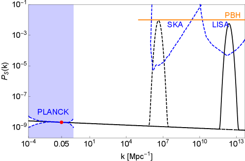
where is the amplitude of the CMB spectrum at the pivot scale and is the spectral tilt given in Eq. (30). The and are free parameters determining the height and width of the Gaussian peak, respectively. To form PBHs on scales smaller than the CMB scale (), the should be enhanced by a factor of about with respect to its value at the CMB scale, which is possible mainly due to the peak amplitude . In Fig. 1, we plot the dependence of Eq. (32) in light of the several observational limits and constraints adopted from Ref. Inomata:2018epa . In particular, the orange line at indicates the required amplitude of power spectra for the PBHs formation Green:2020jor . The figure also implies that the power spectra that have peaks at either or lead to the production of stochastic GW background in the frequency band targeted by the pulsar timing array (PTA) experiments and the space-based interferometers Inomata:2018epa .
Then, to explain the small scale enhancement as parameterized in Eq. (32), we will reconstruct the inflaton potential and the self-coupling functions in Sec. IV from the power spectrum in Eq. (32) and its spectral tilt in Eq. (30).
III.1 Primordial black holes as dark matter
When the curvature perturbations that left the Hubble horizon during inflation reenter the horizon in the RD era, they generate over-dense regions in the universe. The over-density would grow as the universe expands and eventually exceeds a critical value when the comoving size of such region becomes the order of the horizon size. Consequently, all the fluctuations inside the Hubble volume would immediately collapse to form PBHs Zeldovich:1967lct ; Hawking:1971ei ; Carr:1974nx ; Carr:1975qj . The mass of the formed PBHs is assumed to be proportional to the mass inside the Hubble volume, i.e., the horizon mass, at that time Ozsoy:2018flq
| (33) |
where the and denote the solar mass and efficiency of gravitational collapse, respectively. Although the value of depends on the details of gravitational collapse, it has a typical value of Carr:1975qj , which we adopt in this study.
The standard treatment of PBH formation is based on the Press-Schechter model of gravitational collapse Press:1973iz . The energy density fraction of PBHs of mass at the formation to the total mass of the universe is denoted by , where is the energy density of the universe and is the energy density of PBHs. The PBHs would be formed if the density contrast of the over-dense regions dominates a certain threshold value Green:2004wb ; Harada:2013epa ; Musco:2018rwt . The distribution function of the density perturbation is assumed to be governed by the Gaussian statistics. Thus, one can write the production rate of PBHs with mass as follows Ozsoy:2018flq
| (34) |
where the variance represents the coarse-grained density contrast with the smoothing scale and is defined as Young:2014ana ; Ozsoy:2018flq
| (35) |
where and denote the dimensionless power spectra of the primordial comoving curvature perturbations and density perturbations, respectively. For the window function , we adopt the Gaussian function . The current fraction of PBH abundance in total DM today can be determined by Ozsoy:2018flq
| (36) |
where is the current density parameter of DM and
| (37) |
where the effective number of relativistic degrees of freedom is deep inside the RD era and Ade:2013zuv .
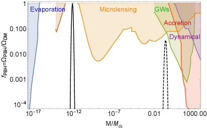
In the left panel of Fig. 2, we plot the current fraction of PBH abundance in total DM today as a function of mass from Eq. (III.1). The figure also presents the currently available constraints from different datasets over various mass ranges as summarized in Ref. Green:2020jor . The result shows that different peak scales in the scalar power spectrum lead to PBHs with different masses. The enhanced power spectra with the and correspond to PBHs with the peak mass around and , the solid and dashed black lines in the figure, respectively. The corresponding peak abundances are and . The peak abundance of PBHs depend on the critical density , and it gets smaller as the value increases and vice versa. For PBHs with the peak mass of and abundances of to form, the critical density contrast should be . Thus, PBHs with the peak mass around can explain almost all the DM in the universe today. When the same value is applied, the PBHs with the peak mass around can make up to of the observed DM abundance today.
III.2 Scalar-induced secondary gravitational waves
The sufficiently large density fluctuations generated during inflation can simultaneously produce a substantial amount of GWs when they reenter the horizon in the RD era Ananda:2006af ; Baumann:2007zm . To investigate the GWs background evolving in the RD era, we assume negligible effects of inflaton field on cosmic evolution after reheating Fu:2019vqc . The equations of motion for the GW amplitude in Fourier space is written as Ananda:2006af ; Baumann:2007zm
| (38) |
where the prime denotes the derivative with respect to conformal time . The conformal Hubble parameter is given in terms of the scale factor , where is the equation-of-state parameter. The source term , which is a convolution of two first-order scalar perturbations at different wave numbers, is given by Ananda:2006af ; Baumann:2007zm
| (39) |
where is the polarization tensor. In the RD era, the scalar part of metric perturbations in Fourier space satisfies Fu:2019vqc
| (40) |
which admits a solution Baumann:2007zm
| (41) |
where is the comoving curvature perturbations, giving rise to the curvature power spectrum of . The power spectrum is given by Eq. (29). Using the Green function method, one obtains the particular solutions for the Eq. (38) as
| (42) |
where the Green’s function obeys the equation of motion
| (43) |
The exact solution to Eq. (43) in the RD era is obtained to be Baumann:2007zm .
The power spectrum of the induced GWs is then defined as
| (44) |
and the fractional energy density per logarithmic wavenumber interval is
| (45) |
where , and the overline indicates the oscillation time average. As the relevant modes reenter the horizon, GWs are assumed to be induced instantaneously Baumann:2007zm . Thus, at the time of horizon reentry, we have ; hence it gets contributions from all scalar modes . One can see from Eqs.(44)–(45) that appears in the integrand in . The main contributions to are from that are closer to . Since the source decays as with , the induced GWs propagate freely soon after horizon reentry and . Thus, well inside the horizon Baumann:2007zm .
After combining Eqs. (39)–(45) and executing a straightforward yet tedious calculation, we obtain the power spectrum of the induced GWs in the RD era as Ananda:2006af ; Baumann:2007zm
| (46) |
where , , and is evaluated upon the horizon exit during inflation. Substituting Eq. (46) into Eq. (45), the fractional energy density of the GWs in the RD era becomes Kohri:2018awv ; Cai:2018dig ; Fu:2019vqc ; Lu:2019sti
| (47) |
where the full expression of is given by
| (48) |
The observed energy densities of GWs today are related to their values after the horizon reentry in the RD era as Inomata:2018epa
| (49) |
where with is the fractional energy density of radiation today, and is the GW energy density at the time of horizon reentry of the mode . A relation between the frequency and comoving wavenumber of induced GWs is
| (50) |
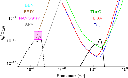
We plot Eq. (49) as a function of frequency in the right panel of Fig. 2 together with the sensitivity curves of various GW experiments and missions targeted at different frequency bands. The figure shows that the GWs with the mHz peak frequency are produced if the primordial power spectrum peaks at ; see the solid black line. The signal of induced GWs falls into the frequency range targeted by the space-borne GW detectors, including LISA Audley:2017drz , Taiji Hu:2017mde , TianQin Luo:2015ght . Similarly, the GWs with the nHz peak frequency can also be produced in the RD era if the primordial power spectrum peaks at ; hence, the predictions of our model can be proved by the PTA experiments, including EPTA Ferdman:2010xq , NANOGrav McLaughlin:2013ira , and SKA Moore:2014lga . Our results tell us that different peak scales in the scalar power spectrum correspond to different frequency of GWs; hence, the signals are probed by different experiments.
IV Inflaton potential and self-coupling functions
In Sec. II, we discussed that the primordial curvature power spectrum could be enhanced due to the self-interaction of the inflaton field and the kinetic coupling between the inflaton and gravity. Then, by proposing the power spectrum with a local Gaussian peak, we estimated the abundance of PBHs and the energy spectrum of induced GWs in Sec. III. Therefore, it is imperative for us to investigate the configuration of inflaton potential and self-coupling function that yields the power spectrum given in Eq. (32). In order words, in this section, we reconstruct the inflaton potential and self-coupling function for our model from the power spectrum and its spectral tilt. Our reconstruction method closely follows Refs. Chiba:2015zpa . We start from Eq. (17) to obtain
| (51) |
where is required. Consequently, we derive from Eqs. (30)–(31)
| (52) |
Since the potential and couplings are functions of the scalar field, we need a relation between and , which we obtain from Eq. (17) as
| (53) |
where and are scalar field values at the end of inflation and the horizon exit of the CMB mode, respectively. Thus, Eqs. (52)–(53) are the key equations for reconstructing and . In this work, we adopt the following form of ,
| (54) |
which is in good agreement with the CMB measurement Ade:2013zuv for and is extensively studied in the literature Chiba:2015zpa . Applying Eq. (54) to Eq. (52), we obtain
| (55) |
which can also be integrated to give
| (56) |
where is a positive constant of integration since . By comparing Eq. (29) with Eq. (32) in the limit, we obtain
| (57) |
where is defined from the end of inflation. The counts the -folds between the horizon exit of a mode during inflation and the end of inflation. The difference indicates how long after the CMB mode exit the horizon, the mode corresponding to PBHs would exit the horizon during inflation. Thus, the varies within an interval as the runs between , where the indicates the smallest scale that exits the horizon during inflation. The CMB data favor Ade:2013zuv . We solve Eq. (56) for using Eq. (57), and the solution is given by
| (58) |
where is an integration constant. The last term in Eq. (58) is negligible compared to the second term if we consider , and . Consequently, from Eq. (12), we obtain
| (59) |
After using Eq. (53), which allows us to interchange with , we get
| (60) | ||||
| (61) |
where
| (62) |
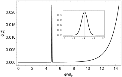
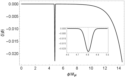
and . The peak in the power spectrum Eq. (32) is, therefore, explained by a local feature of the self-coupling function at . The Eqs. (60) and (61) are our key results of this section and describe the shape of the inflaton potential and self-coupling functions, respectively. It is worth noting here that the potential obtained in Eq. (60) is the same as that in the so-called “T-model” of inflation proposed in Ref. Kallosh:2013maa . In Fig. 3, we plot Eq (61) as functions of the scalar field for positive and negative values of . In conclusion, if the sign of is positive (negative), there appears a bump (dip) in the self-coupling function at . The value of determines the location of a peak in the power spectra. In other words, the peak scale at which the scalar power spectrum is enhanced can be easily adjusted by the value of .
V Conclusion
We have considered the cosmological model Eq. (1) that incorporates the derivative self-interaction of the scalar field and the kinetic coupling between the scalar field and gravity to investigate the formation of PBHs and induced GWs from inflationary quantum fluctuations. We have derived the inflationary observables and showed in Sec. II that such additional interactions leave their imprints in the primordial power spectrum hence the spectral tilts, as well as the tensor-to-scalar ratio. In particular, the power spectrum of the scalar perturbations Eq. (29) is enhanced compared to the case in GR, whereas the tensor spectrum Eq. (22) is suppressed. If the power spectra are enhanced on scales smaller than the CMB pivot scale, they lead to the formation of PBHs and the production of GWs in the RD era.
The enhancement of the power spectrum is often associated with the local feature of inflaton potentials. However, not every inflaton potentials induce such enhancement; hence a certain degree of fine-tuning is needed. To avoid such fine-tuning, we have specified and proposed the form of the power spectrum in Sec. III instead. The proposed power spectrum is parameterized with a local smooth Gaussian peak, as is seen in Eq. (32) and Fig. 1. The numerical results of Sec. III are presented in Fig. 2. Our findings can be summarized as follows. With the enhanced power spectra, PBHs are produced with the peak mass around and . The corresponding peak abundances are and . As a result, the PBHs with the peak mass around can explain almost all the DM in the universe today, while only up to of the observed DM can be explained by the PBHs with the peak mass around . Moreover, the induced GWs with the peak frequency around mHz and nHz can be produced. The induced GWs in our model can be tested by both the space-borne GW detectors and PTA observations.
To explain the enhancement in the power spectrum, we have reconstructed the inflaton potential and self-interaction functions in Sec. IV from the proposed power spectrum and its spectral tilt. The main results of Sec. IV are, therefore, Eqs. 60 and (61). The inflationary predictions of our model are consistent with Planck data Ade:2013zuv . The reconstructed inflaton potential has the same form as the so-called “ T-model” of inflation Kallosh:2013maa . The enhancement in the power spectrum can be explained by the local feature of the self-coupling function of the inflaton field. Depending on the sign, there appears a peak or dip in the small field range of the coupling functions. The precise location of the peak is adjusted by how long after the CMB mode the relevant mode that produces a peak in the power spectra leaves the horizon during inflation.
In conclusion, for our model, the PBHs and GWs are successfully produced as long as the primordial curvature power spectrum is enhanced on scales smaller than the CMB pivot scale. The enhancement mechanism is then explained by the local feature, either a peak or dip, of the inflaton self-coupling function rather than the local feature of the inflaton potential.
Acknowledgements.
PC and GT are supported by Ministry of Science and Technology (MoST) under grant No. 109-2112-M-002-019. SK was supported by the National Research Foundation of Korea (NRF-2016R1D1A1B04932574, NRF-2021R1A2C1005748) and by the 2020 scientific promotion porgram funded by Jeju National University.References
- (1) A. H. Guth, “The Inflationary Universe: A Possible Solution to the Horizon and Flatness Problems,” Phys. Rev. D 23, 347 (1981) [Adv. Ser. Astrophys. Cosmol. 3, 139 (1987)];
- (2) A. D. Linde, “A New Inflationary Universe Scenario: A Possible Solution of the Horizon, Flatness, Homogeneity, Isotropy and Primordial Monopole Problems,” Phys. Lett. 108B, 389 (1982) [Adv. Ser. Astrophys. Cosmol. 3, 149 (1987)]; A. D. Linde, “Chaotic Inflation,” Phys. Lett. 129B, 177 (1983);
- (3) A. Albrecht and P. J. Steinhardt, “Cosmology for Grand Unified Theories with Radiatively Induced Symmetry Breaking,” Phys. Rev. Lett. 48, 1220 (1982) [Adv. Ser. Astrophys. Cosmol. 3, 158 (1987)];
- (4) K. Sato, “First Order Phase Transition of a Vacuum and Expansion of the Universe,” Mon. Not. Roy. Astron. Soc. 195, 467 (1981);
- (5) V. F. Mukhanov and G. V. Chibisov, “Quantum Fluctuations and a Nonsingular Universe,” JETP Lett. 33, 532 (1981) [Pisma Zh. Eksp. Teor. Fiz. 33, 549 (1981)];
- (6) S. W. Hawking, “The Development of Irregularities in a Single Bubble Inflationary Universe,” Phys. Lett. 115B, 295 (1982);
- (7) A. A. Starobinsky, “Dynamics of Phase Transition in the New Inflationary Universe Scenario and Generation of Perturbations,” Phys. Lett. 117B, 175 (1982);
- (8) A. H. Guth and S. Y. Pi, “Fluctuations in the New Inflationary Universe,” Phys. Rev. Lett. 49, 1110 (1982);
- (9) J. M. Bardeen, P. J. Steinhardt and M. S. Turner, “Spontaneous Creation of Almost Scale - Free Density Perturbations in an Inflationary Universe,” Phys. Rev. D 28, 679 (1983);
- (10) H. Kodama and M. Sasaki, “Cosmological Perturbation Theory,” Prog. Theor. Phys. Suppl. 78, 1 (1984);
- (11) P. A. R. Ade et al. [Planck Collaboration], “Planck 2013 results. XVI. Cosmological parameters,” Astron. Astrophys. 571, A16 (2014); P. A. R. Ade et al. [Planck Collaboration], “Planck 2015 results. XIII. Cosmological parameters,” Astron. Astrophys. 594, A13 (2016); N. Aghanim et al. [Planck Collaboration], “Planck 2018 results. VI. Cosmological parameters,” arXiv:1807.06209 [astro-ph.CO];
- (12) A. A. Starobinsky, “Spectrum of relict gravitational radiation and the early state of the universe,” JETP Lett. 30 (1979), 682-685;
- (13) B. Allen, “The Stochastic Gravity Wave Background in Inflationary Universe Models,” Phys. Rev. D 37 (1988), 2078;
- (14) V. Sahni, “The Energy Density of Relic Gravity Waves From Inflation,” Phys. Rev. D 42 (1990), 453-463;
- (15) S. Matarrese, O. Pantano and D. Saez, “A General relativistic approach to the nonlinear evolution of collisionless matter,” Phys. Rev. D 47 (1993), 1311-1323; S. Matarrese, O. Pantano and D. Saez, “General relativistic dynamics of irrotational dust: Cosmological implications,” Phys. Rev. Lett. 72 (1994), 320-323; S. Matarrese, S. Mollerach and M. Bruni, “Second order perturbations of the Einstein-de Sitter universe,” Phys. Rev. D 58 (1998), 043504; C. Carbone and S. Matarrese, “A Unified treatment of cosmological perturbations from super-horizon to small scales,” Phys. Rev. D 71 (2005), 043508;
- (16) H. Noh and J. c. Hwang, “Second-order perturbations of the Friedmann world model,” Phys. Rev. D 69 (2004), 104011;
- (17) K. Nakamura, “Second-order gauge invariant cosmological perturbation theory: Einstein equations in terms of gauge invariant variables,” Prog. Theor. Phys. 117 (2007), 17-74;
- (18) K. N. Ananda, C. Clarkson and D. Wands, “The Cosmological gravitational wave background from primordial density perturbations,” Phys. Rev. D 75 (2007), 123518;
- (19) D. Baumann, P. J. Steinhardt, K. Takahashi and K. Ichiki, “Gravitational Wave Spectrum Induced by Primordial Scalar Perturbations,” Phys. Rev. D 76 (2007), 084019;
- (20) L. Alabidi, K. Kohri, M. Sasaki and Y. Sendouda, “Observable Spectra of Induced Gravitational Waves from Inflation,” JCAP 09 (2012), 017;
- (21) K. Kohri and T. Terada, “Semianalytic calculation of gravitational wave spectrum nonlinearly induced from primordial curvature perturbations,” Phys. Rev. D 97 (2018) no.12, 123532;
- (22) R. g. Cai, S. Pi and M. Sasaki, “Gravitational Waves Induced by non-Gaussian Scalar Perturbations,” Phys. Rev. Lett. 122 (2019) no.20, 201101; R. G. Cai, S. Pi, S. J. Wang and X. Y. Yang, “Resonant multiple peaks in the induced gravitational waves,” JCAP 05 (2019), 013; S. Pi and M. Sasaki, “Gravitational Waves Induced by Scalar Perturbations with a Lognormal Peak,” JCAP 09 (2020), 037;
- (23) C. Fu, P. Wu and H. Yu, “Scalar induced gravitational waves in inflation with gravitationally enhanced friction,” Phys. Rev. D 101 (2020) no.2, 023529;
- (24) K. Inomata and T. Nakama, “Gravitational waves induced by scalar perturbations as probes of the small-scale primordial spectrum,” Phys. Rev. D 99 (2019) no.4, 043511;
- (25) K. Inomata, K. Kohri, T. Nakama and T. Terada, “Gravitational Waves Induced by Scalar Perturbations during a Gradual Transition from an Early Matter Era to the Radiation Era,” JCAP 10 (2019), 071;
- (26) G. Domènech, S. Pi and M. Sasaki, “Induced gravitational waves as a probe of thermal history of the universe,” JCAP 08 (2020), 017;
- (27) Y. B. ;. N. Zel’dovich, I. D., “The Hypothesis of Cores Retarded during Expansion and the Hot Cosmological Model,” Soviet Astron. AJ (Engl. Transl. ), 10 (1967), 602;
- (28) S. Hawking, “Gravitationally collapsed objects of very low mass,” Mon. Not. Roy. Astron. Soc. 152 (1971), 75;
- (29) B. J. Carr and S. W. Hawking, “Black holes in the early Universe,” Mon. Not. Roy. Astron. Soc. 168 (1974), 399-415;
- (30) B. J. Carr, “The Primordial black hole mass spectrum,” Astrophys. J. 201 (1975), 1-19;
- (31) B. J. Carr, K. Kohri, Y. Sendouda and J. Yokoyama, “New cosmological constraints on primordial black holes,” Phys. Rev. D 81 (2010), 104019;
- (32) P. Ivanov, P. Naselsky and I. Novikov, “Inflation and primordial black holes as dark matter,” Phys. Rev. D 50 (1994), 7173-7178;
- (33) P. H. Frampton, M. Kawasaki, F. Takahashi and T. T. Yanagida, “Primordial Black Holes as All Dark Matter,” JCAP 04 (2010), 023;
- (34) K. M. Belotsky, A. D. Dmitriev, E. A. Esipova, V. A. Gani, A. V. Grobov, M. Y. Khlopov, A. A. Kirillov, S. G. Rubin and I. V. Svadkovsky, “Signatures of primordial black hole dark matter,” Mod. Phys. Lett. A 29 (2014) no.37, 1440005;
- (35) B. Carr, F. Kuhnel and M. Sandstad, “Primordial Black Holes as Dark Matter,” Phys. Rev. D 94 (2016) no.8, 083504;
- (36) K. Inomata, M. Kawasaki, K. Mukaida, Y. Tada and T. T. Yanagida, “Inflationary Primordial Black Holes as All Dark Matter,” Phys. Rev. D 96 (2017) no.4, 043504;
- (37) B. Carr and F. Kuhnel, “Primordial Black Holes as Dark Matter: Recent Developments,” Ann. Rev. Nucl. Part. Sci. 70 (2020), 355-394;
- (38) R. J. Adler, P. Chen and D. I. Santiago, “The Generalized uncertainty principle and black hole remnants,” Gen. Rel. Grav. 33 (2001), 2101-2108;
- (39) P. Chen and R. J. Adler, “Black hole remnants and dark matter,” Nucl. Phys. B Proc. Suppl. 124 (2003), 103-106;
- (40) P. Chen, “Inflation induced Planck-size black hole remnants as dark matter,” New Astron. Rev. 49 (2005), 233-239;
- (41) F. Scardigli, C. Gruber and P. Chen, “Black Hole Remnants in the Early Universe,” Phys. Rev. D 83 (2011), 063507;
- (42) I. Dalianis and G. Tringas, “Primordial black hole remnants as dark matter produced in thermal, matter, and runaway-quintessence postinflationary scenarios,” Phys. Rev. D 100 (2019) no.8, 083512;
- (43) S. Bird, I. Cholis, J. B. Muñoz, Y. Ali-Haïmoud, M. Kamionkowski, E. D. Kovetz, A. Raccanelli and A. G. Riess, “Did LIGO detect dark matter?,” Phys. Rev. Lett. 116 (2016) no.20, 201301;
- (44) M. Sasaki, T. Suyama, T. Tanaka and S. Yokoyama, “Primordial Black Hole Scenario for the Gravitational-Wave Event GW150914,” Phys. Rev. Lett. 117 (2016) no.6, 061101 [erratum: Phys. Rev. Lett. 121 (2018) no.5, 059901];
- (45) J. M. Ezquiaga, J. Garcia-Bellido and E. Ruiz Morales, “Primordial Black Hole production in Critical Higgs Inflation,” Phys. Lett. B 776 (2018), 345-349;
- (46) S. S. Mishra and V. Sahni, “Primordial Black Holes from a tiny bump/dip in the Inflaton potential,” JCAP 04 (2020), 007;
- (47) D. Y. Cheong, S. M. Lee and S. C. Park, “Primordial black holes in Higgs- inflation as the whole of dark matter,” JCAP 01 (2021), 032;
- (48) M. P. Hertzberg and M. Yamada, “Primordial Black Holes from Polynomial Potentials in Single Field Inflation,” Phys. Rev. D 97 (2018) no.8, 083509;
- (49) Y. Lu, Y. Gong, Z. Yi and F. Zhang, “Constraints on primordial curvature perturbations from primordial black hole dark matter and secondary gravitational waves,” JCAP 12 (2019), 031;
- (50) Z. Yi, Q. Gao, Y. Gong and Z. h. Zhu, “Primordial black holes and scalar-induced secondary gravitational waves from inflationary models with a noncanonical kinetic term,” Phys. Rev. D 103 (2021) no.6, 063534;
- (51) Q. Gao, Y. Gong and Z. Yi, “Primordial black holes and secondary gravitational waves from natural inflation,” [arXiv:2012.03856 [gr-qc]];
- (52) Z. Yi, Y. Gong, B. Wang and Z. h. Zhu, “Primordial black holes and secondary gravitational waves from the Higgs field,” Phys. Rev. D 103 (2021) no.6, 063535;
- (53) J. Lin, Q. Gao, Y. Gong, Y. Lu, C. Zhang and F. Zhang, “Primordial black holes and secondary gravitational waves from and inflation,” Phys. Rev. D 101 (2020) no.10, 103515;
- (54) G. Tumurtushaa, “Inflation with Derivative Self-interaction and Coupling to Gravity,” Eur. Phys. J. C 79, no.11, 920 (2019);
- (55) B. Bayarsaikhan, S. Koh, E. Tsedenbaljir and G. Tumurtushaa, “Constraints on dark energy models from the Horndeski theory,” JCAP 11 (2020), 057;
- (56) G. W. Horndeski, “Second-order scalar-tensor field equations in a four-dimensional space,” Int. J. Theor. Phys. 10, 363-384 (1974);
- (57) C. Deffayet, X. Gao, D. A. Steer and G. Zahariade, “From k-essence to generalised Galileons,” Phys. Rev. D 84 (2011), 064039;
- (58) T. Kobayashi, M. Yamaguchi and J. Yokoyama, “Generalized G-inflation: Inflation with the most general second-order field equations,” Prog. Theor. Phys. 126, 511 (2011);
- (59) X. Gao, T. Kobayashi, M. Yamaguchi and J. Yokoyama, “Primordial non-Gaussianities of gravitational waves in the most general single-field inflation model,” Phys. Rev. Lett. 107, 211301 (2011);
- (60) X. Gao, T. Kobayashi, M. Shiraishi, M. Yamaguchi, J. Yokoyama and S. Yokoyama, “Full bispectra from primordial scalar and tensor perturbations in the most general single-field inflation model,” PTEP 2013, 053E03 (2013);
- (61) C. Deffayet and D. A. Steer, “A formal introduction to Horndeski and Galileon theories and their generalizations,” Class. Quant. Grav. 30 (2013), 214006;
- (62) C. Germani and A. Kehagias, “New Model of Inflation with Non-minimal Derivative Coupling of Standard Model Higgs Boson to Gravity,” Phys. Rev. Lett. 105 (2010), 011302;
- (63) C. Germani and A. Kehagias, “Cosmological Perturbations in the New Higgs Inflation,” JCAP 05 (2010), 019;
- (64) S. Tsujikawa, “Observational tests of inflation with a field derivative coupling to gravity,” Phys. Rev. D 85 (2012), 083518;
- (65) N. Yang, Q. Gao and Y. Gong, “Inflation with non-minimally derivative coupling,” Int. J. Mod. Phys. A 30 (2015) no.28n29, 1545004;
- (66) N. Yang, Q. Fei, Q. Gao and Y. Gong, “Inflationary models with non-minimally derivative coupling,” Class. Quant. Grav. 33 (2016) no.20, 205001;
- (67) S. Sato and K. i. Maeda, “Hybrid Higgs Inflation: The Use of Disformal Transformation,” Phys. Rev. D 97 (2018) no.8, 083512;
- (68) K. Kohri and T. Terada, “Solar-Mass Primordial Black Holes Explain NANOGrav Hint of Gravitational Waves,” Phys. Lett. B 813 (2021), 136040;
- (69) A. M. Green and B. J. Kavanagh, “Primordial Black Holes as a dark matter candidate,” J. Phys. G 48 (2021) no.4, 4;
- (70) O. Özsoy, S. Parameswaran, G. Tasinato and I. Zavala, “Mechanisms for Primordial Black Hole Production in String Theory,” JCAP 07 (2018), 005;
- (71) W. H. Press and P. Schechter, “Formation of galaxies and clusters of galaxies by selfsimilar gravitational condensation,” Astrophys. J. 187 (1974), 425-438;
- (72) A. M. Green, A. R. Liddle, K. A. Malik and M. Sasaki, “A New calculation of the mass fraction of primordial black holes,” Phys. Rev. D 70 (2004), 041502;
- (73) T. Harada, C. M. Yoo and K. Kohri, “Threshold of primordial black hole formation,” Phys. Rev. D 88 (2013) no.8, 084051 [erratum: Phys. Rev. D 89 (2014) no.2, 029903];
- (74) I. Musco, “Threshold for primordial black holes: Dependence on the shape of the cosmological perturbations,” Phys. Rev. D 100 (2019) no.12, 123524;
- (75) S. Young, C. T. Byrnes and M. Sasaki, “Calculating the mass fraction of primordial black holes,” JCAP 07 (2014), 045;
- (76) P. Amaro-Seoane et al. [LISA], “Laser Interferometer Space Antenna,” [arXiv:1702.00786 [astro-ph.IM]];
- (77) W. R. Hu and Y. L. Wu, “The Taiji Program in Space for gravitational wave physics and the nature of gravity,” Natl. Sci. Rev. 4 (2017) no.5, 685-686;
- (78) J. Luo et al. [TianQin], “TianQin: a space-borne gravitational wave detector,” Class. Quant. Grav. 33 (2016) no.3, 035010;
- (79) R. D. Ferdman, R. van Haasteren, C. G. Bassa, M. Burgay, I. Cognard, A. Corongiu, N. D’Amico, G. Desvignes, J. W. T. Hessels and G. H. Janssen, et al. “The European Pulsar Timing Array: current efforts and a LEAP toward the future,” Class. Quant. Grav. 27 (2010), 084014; G. Hobbs, A. Archibald, Z. Arzoumanian, D. Backer, M. Bailes, N. D. R. Bhat, M. Burgay, S. Burke-Spolaor, D. Champion and I. Cognard, et al. “The international pulsar timing array project: using pulsars as a gravitational wave detector,” Class. Quant. Grav. 27 (2010), 084013; G. Hobbs, “The Parkes Pulsar Timing Array,” Class. Quant. Grav. 30 (2013), 224007;
- (80) M. A. McLaughlin, “The North American Nanohertz Observatory for Gravitational Waves,” Class. Quant. Grav. 30 (2013), 224008;
- (81) C. J. Moore, R. H. Cole and C. P. L. Berry, “Gravitational-wave sensitivity curves,” Class. Quant. Grav. 32 (2015) no.1, 015014;
- (82) E. J. Copeland, E. W. Kolb, A. R. Liddle and J. E. Lidsey, “Reconstructing the inflation potential, in principle and in practice,” Phys. Rev. D 48 (1993), 2529-2547; J. E. Lidsey, A. R. Liddle, E. W. Kolb, E. J. Copeland, T. Barreiro and M. Abney, “Reconstructing the inflation potential : An overview,” Rev. Mod. Phys. 69 (1997), 373-410; R. Easther and W. H. Kinney, “Monte Carlo reconstruction of the inflationary potential,” Phys. Rev. D 67 (2003), 043511; T. Chiba, “Reconstructing the inflaton potential from the spectral index,” PTEP 2015 (2015) no.7, 073E02; J. Lin, Q. Gao and Y. Gong, “The reconstruction of inflationary potentials,” Mon. Not. Roy. Astron. Soc. 459 (2016) no.4, 4029-4037; S. Koh, B. H. Lee and G. Tumurtushaa, “Reconstruction of the Scalar Field Potential in Inflationary Models with a Gauss-Bonnet term,” Phys. Rev. D 95 (2017) no.12, 123509; Q. Gao and Y. Gong, “Reconstruction of extended inflationary potentials for attractors,” Eur. Phys. J. Plus 133 (2018) no.11, 491;
- (83) R. Kallosh and A. Linde, “Non-minimal Inflationary Attractors,” JCAP 10 (2013), 033; R. Kallosh and A. Linde, “Universality Class in Conformal Inflation,” JCAP 07 (2013), 002.