Pricing Social Visibility Service in Online Social Networks: Modeling and Algorithms
Abstract
Online social networks (OSNs) such as YoutTube, Instagram, Twitter, Facebook, etc., serve as important platforms for users to share their information or content to friends or followers. Often times, users want to enhance their social visibility, as it can make their contents, i.e., opinions, videos, pictures, etc., attract attention from more users, which in turn may bring higher commercial benefit to them. Motivated by this, we propose a mechanism, where the OSN operator provides a “social visibility boosting service” to incentivize “transactions” between requesters (users who seek to enhance their social visibility via adding new “neighbors”) and suppliers (users who are willing to be added as a new “neighbor” of any requester when certain “rewards” is provided). We design a posted pricing scheme for the OSN provider to charge the requesters who use such boosting service, and reward the suppliers who contribute to such boosting service. The OSN operator keeps a fraction of the payment from requesters and distribute the remaining part to participating suppliers “fairly” via the Shapley value. The objective of the OSN provider is to select the price and supplier set to maximize the total amount of revenue under the budget constraint of requesters. We first show that the revenue maximization problem is not simpler than an NP-hard problem. We then decomposed it into two sub-routines, where one focuses on selecting the optimal set of suppliers, and the other one focuses on selecting the optimal price. We prove the hardness of each sub-routine, and eventually design a computationally efficient approximation algorithm to solve the revenue maximization problem with provable theoretical guarantee on the revenue gap. We conduct extensive experiments on four public datasets to validate the superior performance of our proposed algorithms.
I Introduction
OSNs such as YouTube, Instagram, Twitter, Facebook, etc., serve as important platforms for users to share their information or content to friends or followers, e.g., users in Facebook can share their opinions or status to their friends via the friendship network. Users in YouTube can share their videos to their subscribers via the subscriber network. A user’s friends or followers can further share the information or content of this user to their friends or followers. Hence, the information or content of a user can be propagated to his direct friends or followers, or even multi-hop friends or followers. In other words, a user is “socially visible” to his direct friends or followers and some multi-hop friends or followers.
Often times, users want to enhance their social visibility, as it can make their contents, i.e., opinions, videos, pictures, etc., attract attention from more users, which in turn may bring higher commercial benefit to them. We call a user who wants to enhance social visibility as a requester. One way to enhance a requester’s social visibility is to attract some new friends or followers. It is well known that the OSN is under the “rich gets richer” phenomenon, which makes it difficult for requesters, especially those with low social visibility, to attract new friends or followers. But when finical incentive is provided, some users will be willing to be added as requesters’ new friends or followers. We call such users as suppliers. Hence, requesters can provide financial incentives to enhance their social visibility. This paper aims to answer the following fundamental question: How to set appropriate financial incentives to incentivize the “transaction” between requesters and suppliers?
We propose a mechanism, where the OSN operator provides a “social visibility boosting service” to incentivize the transaction between requesters and suppliers. The visibility boosting service is sold via a posted normalized pricing scheme , where and . Here, is the price of per unit social visibility improvement that the OSN operator charges a participating requester, and is the price of per unit contribution in improving social visibility of participating requesters that the OSN operator pays to a participating supplier. We consider the case that each participating supplier adds links to all participating requesters and requesters has a budget to add new friends or followers. Requesters and suppliers decide whether to participate or not by comparing their valuations to the posted prices . We consider a proportional transaction fee scheme, i.e., the OSN operator keeps a fraction of the payment from requesters, and distribute the remaining part (we call it “reward”) to suppliers. The objectives of the OSN operator are: (1) select the price and supplier set so to maximize the total amount of transaction fees or revenue; (2) divide the reward “fairly” to all suppliers.
Each of the above two objectives is technically challenging to achieve. One can observe that selecting the price and supplier set involves a mixed optimization problem, i.e., with both continuous decision variables, i.e., and , and set decision variables, i.e., supplier set. This implies that gradient based optimization methods does not work for this problem. To illustrate the hardness of this optimization problem, consider the case where and are given and our objective is to select the supplier set. The number of suppliers may exceed the budget and the OSN operator needs to select at most suppliers from them. Due to network externality effect of social visibility, suppliers are not independent in enhancing the social visibility of a requester. In other words, the total improvement of social visibility by two suppliers does not equal to the total improvement of social visibility made by each individual supplier. As one will see in Section III, this dependency among suppliers makes this simplified problem NP-hard already. Also, this dependency among suppliers also makes it challenging to fairly divide the reward to suppliers. We address these challenges and our contributions are:
-
•
We formulate a mathematical model to quantify social visibility. To the best of our knowledge, we are the first to propose a posted pricing scheme and formulate a revenue maximization problem for visibility boosting service.
-
•
We prove that the revenue maximization problem is not simpler than an NP-hard problem. We decomposed it into two sub-routines, where one focuses on selecting the optimal set of suppliers, and the other focuses on selecting the optimal price. We prove the hardness of each sub-problem and propose approximation algorithms for each sub-problem with theoretical guarantees on the approximation ratio, i.e., a ratio of for the first sub-routine and a ratio which can be make arbitrarily small via increasing the computational complexity of searching for the second sub-routine. Finally, we prove that combining these approximation algorithms, we obtain an algorithm to solve the revenue maximization problem with provable theoretical guarantee on the revenue gap.
-
•
We show how to divide the reward to suppliers fairly via the Shapley value concept. We conduct experiments on real-world social network datasets, and the results validate the effectiveness and efficiency of our algorithms.
II Model & Problem Formulation
II-A The Social Visibility Model
Online Social Network. Consider an OSN which is characterized by an unweighted and directed graph , where denotes a set of users and denotes a set of edges between users. Note that a directed edge from user to user is denoted by . For example, this social network model captures the Twitter social network, the Facebook social network (each undirected edge between user and is represented by two directed edges and ). We focus on the case that there is no self-loop edges, i.e., .
Social Visibility. Denote a directed path in graph as
where , and . Note that captures that there is no self-loop edges or circles in the path. Denote a set of all directed edges on path as
Let denote the length (or number of hops) of path , which can be expressed as . Let denote the set of all directed paths (without circles) from user to user in . Let denote the distance from user to user in graph . We define as the length of the shortest path from to , i.e.,
Namely, when there is no directed path from to , the distance from to is infinite. Based on distance between nodes, we define user being -visible to user if
The -visible set of user is defined as the set of all users to whom user is -visible, formally
Let denote the social visibility threshold of an OSN. This notion of social visibility threshold captures that the information of a user can be propagated to its followers and its followers may further propagate their own follower and so on so forth. Namely, user is not visible to users whose distance to user is larger than . For example, models that each user is only visible to its own followers, while models that each user is visible to its own one-hop and two-hop followers. Based on , we define the notation of visibility.
Definition 1.
The visibility of user is the cardinality of his -visible set.
For example, Fig. 1 shows that, user ’s -visible set is and -visible set is . With a social visibility threshold of , user ’s visibility is .

II-B Pricing The Social Visibility
The pricing scheme. A “requester” is a user in the set who seeks to increase his visibility by requesting other users to be his new incoming neighbors. Let denote a set of all requesters. A “supplier” is a user in the set who is willing to be a new incoming neighbor of any requester. Let denote a set of all suppliers. For the ease of presentation, we assume that , this captures that a user can not be both requester and supplier. We consider the general case that there are some users who are neither requesters nor suppliers, i.e., . The OSN operator provides a “social visibility boosting service” to incentivize the “transaction” between requesters and suppliers. The visibility improvement service is sold at via a posted pricing scheme , where and . Here, is the price of per unit social visibility improvement that the OSN operator charges a participating requester (i.e., requesters who use this social visibility boosting service), and is the price of per unit contribution in improving social visibility of participating requesters that the OSN operator pays to a participating supplier (i.e., add links to requesters). We consider the case that each participating supplier will add links to all participating requesters.
Requesters’ decision model. Each requester has a per unit valuation (i.e., the per unit price that requester is willing to pay) of on the improvement of his social visibility. A requester will use the social visibility boosting service if his per unit valuation is not below the per unit price, i.e., . Let denote a set of all participating requesters under price , formally
Due to financial budget on boosting service, each requester can afford to add at most incoming neighbors.
Supplier’s decision model. Each supplier has a per unit valuation (i.e., the per unit price that supplier is willing to participate) of on the per unit contribution in improving social visibility of participating requesters. Let denote a set participating suppliers, where . Let denote the new graph after adding edges from participating suppliers to participating requesters. can be expressed as:
Let denote the improvement of social visibility of requester . It can be expressed as:
Then, the total improvement of social visibility of all participating requesters is
In other words, all participating suppliers make a total contribution of in social visibility enhancement. Quantifying among participating suppliers is a non-trivial problem. There are two underlying challenges: (1) some participating suppliers may have a larger number of follower while others may have a small number of followers; (2) the network structure poses an externality effect, causing the contribution of participating suppliers being correlated. To incentivize suppliers to participate, one needs to divide fairly among suppliers. Let denote a “fair” division mechanism, which prescribes a contribution denoted by for each participating supplier. In order to avoid distracting readers, we defer the detail explanation of to the next section. Given the fair division mechanism , a supplier is willing to participant in the social visibility boosting service if his per unit valuation does not exceed the per unit price that the OSN operator pays, i.e., . Let denote a set of all potential participating suppliers under price , formally
Optimal pricing to maximize revenue. Under the posted pricing scheme, the total payment made by all requesters to the OSN operator can be expressed as:
The total payment made by the OSN operator to all participating suppliers can be expressed as:
The revenue of the OSN operator is therefore:
We consider a proportional transaction fee scheme, i.e., the OSN operator keeps a fraction of , where . This is equivalent to imposing . We next formulate a revenue maximization problem for the OSN operator to select and .
Problem 1 (Optimal pricing to maximize revenue).
Select and to maximize the revenue of the OSN operator:
One can observe that the Problem 1 is a mixed optimization problem, i.e., with both continuous and set decision variables.
III Algorithms For Optimal Pricing
We first show that Problem 1 is not simpler than a NP-hard problem. Then we decomposed Problem 1 into two sub-problems. We prove the hardness of each sub-problem and propose approximation algorithms for each sub-problem. Finally, we prove that combining these approximation algorithms, we obtain an algorithm to solve Problem 1 with provable theoretical guarantee on the revenue gap. Due to page limit, all technical proofs to lemmas and theorems are presented in our supplementary file [1].
III-A Hardness Analysis
Hardness analysis. Recall that Problem 1 is a mixed optimization problem, i.e., with both continuous decision variables, i.e., and , and set decision variables, i.e., . This implies that gradient based optimization methods does not work for Problem 1. To illustrate the hardness of Problem 1, we consider a sub-problem of Problem 1 with given pricing parameters , which is stated as follows:
Problem 2 (Optimal supplier set ).
Given and such that with , select to maximize the revenue of the OSN operator:
Namely, Problem 2 only selects the optimal set of suppliers to maximize the revenue of the OSN operator. Note that the set of potential participating suppliers is determined as is given. In the following theorem, we analyze its hardness.
Theorem 1.
Problem 2 is NP-hard to solve.
Theorem 1 states that it is NP-hard to locate the optimal set of supplier for Problem 2. In other words, it is computationally expensive to locate the exact optimal set of supplier for Problem 2. Note that Problem 2 is a sub-problem of Problem 1. Namely, Problem 1 is harder than Problem 2. And therefore, locating the exact optimal solution for Problem 1 is computationally expensive. We resort to design approximation algorithms for Problem 1 with theoretical guarantee.
Our approach. To address Problem 1, we decompose it into two sub-problems, which each sub-problem serves as a subroutine. In particular, Problem 2 is the first sub-problem. As Theorem 1 shows that Problem 2 is NP-hard, we aim to design an approximation algorithm which we denote as OptSupplierSet (its detail is postpone to Section III-B). Algorithm OptSupplierSet takes the prices as an input, and returns an approximately optimal set of suppliers under . We use OptSupplierSet as an oracle to search for the optimal pricing parameter . Formally, we aim to solve the following sub-problem:
Problem 3 (Optimal price ).
Given the algorithm OptSupplierSet, select so to maximize the revenue of the OSN operator:
Note that OptSupplierSet returns an approximately optimal set of suppliers for each given , Problem 3 returns an approximately optimal price. We aim to design an approximation algorithm for Problem 3, which we denote as OptPrice (its detail is postpone to Section III-C). One needs to supply OptPrice with algorithm OptSupplierSet, and OptPrice returns an approximately optimal . We next proceed to present the design and analysis of OptSupplierSet and OptPrice.
III-B Design & Analysis of OptSupplierSet
Submodular analysis. First, note that once and are given, the set of participating requesters and the set of potential participating suppliers are given. Our objective is to select with the constraint , so as to maximize the objective function of Problem 2, i.e., revenue , where and are given and . When , the can be derived as:
where and are the start node and the end node of each link . Based on the above closed-form expression of , the following theorem shows the sub-modularity and monotonicity of with respect to .
Theorem 2.
Given and , such that , the revenue is monotonously increasing and submodular with respect to .
Theorem 2 states that is monotonously increasing and submodular with respect to for each given and with .
The OptSupplierSet algorithm. Based on Theorem 2, Algorithm 1 specifies a greedy algorithm to implement OptSupplierSet. The core idea of Algorithm 1 is that we select suppliers one by one. Each time we select the supplier that achieves the largest marginal improvement in the revenue.
The following theorem presents the theoretical guarantees for Algorithm 1.
Theorem 3.
Given and , such that . The output of Algorithm 1 satisfies: We have
where denotes the optimal set of suppliers via exhaustive search.
III-C Design & Analysis of OptPrice
Perfect search. Now we consider the case that given OptSupplierSet outlined in Algorithm 1, we can obtain exact optimal price for Problem 3. The objective is to understand the impact of the approximate optimal supplier set returned by OptSupplierSet on the optimal price . We state this impact in the following theorem.
Theorem 4.
Theorem 4 states that with OptSupplierSet outlined in Algorithm 1, an optimal solution of Problem 3 attains an approximation ratio of of the optimal solution of Problem 1. However, the optimal solution of Problem 3 is not easy to obtain. One challenge is that the closed-form expression of the objective function of Problem 3, i.e., , is not available, and its gradient is not available as well. Thus, we resort to gradient-free algorithms to solve Problem 3, in particular, the discretized search method. We leave it as a future work to study other advanced methods such as Monte Carlo optimization to address this challenge.
Discretized search. Note that . We therefore discretize the domain of , i.e., , uniformly:
where is price search step the The OSN operator can control to adjust the number of points in . The OSN operator can use exhaustive search method to select the optimal price , denoted by . Algorithm 2 outlines this discretized search algorithm. We denote . The set of supplier is then The following theorem states the theoretical guarantee of this method.
Theorem 5.
Suppose is -Lipschitz with respect to , then the output of Algorithm 2 satisfies
Theorem 5 states that when is -Lipschitz with respect to , the revenue gap between the discretized search method and the perfect search method is bounded by . An attractive of this algorithm is that the OSN operator can make this gap arbitrarily small by selection small enough . Selecting smaller leads to a larger computational complexity. Thus, Theorem 5 serves as a building block for an OSN operator to make a tradeoff between computational complexity and revenue. Combining them all, we prove the revenue gap between the pricing searched by the discretized search method and the optimal pricing of Problem 1.
IV Algorithms for Fair Division of Contribution
Our results so far can locate the approximate optimal price and supplier set, i.e., . The remaining issue is how to divide the contribution among participating suppliers fairly. As we mentioned in Section II that a “fair” division mechanism is important to incentivize the participation of suppliers. Given the approximate optimal solution , the OSN operator needs to divide a total contribution of social visibility improvement among all participating suppliers. Note that the naive equal division, i.e., participating suppliers equally share is not a fair division. This is because: (1) some participating suppliers may have a larger number of follower while others may have a small number of followers; (2) the network structure poses an externality effect, causing the contribution of participating suppliers being correlated. To achieve fair division, we apply the Shapley value [2] to divide . Formally, each participating supplier gets the following share of profit:
Readers can refer to [2] for why Shapley value achieves fair division.
One challenge is that the computational complexity of evaluating is exponential in the cardinality of . To address this computational challenge, we propose to use the sampling algorithm [3] to approximate . Let denote an ordering of the participating suppliers, where and denotes the participating supplier in the -th order. Denote the set of players ranked before player in the order as
Based on [3], the can be rewritten as
| (1) |
where denotes a set of all participating suppliers, and denotes a uniform distribution over . Based on Equation 1, Algorithm 3 outlines a sampling algorithm to approximate .
The following theorem states theoretical guarantee for the approximation accuracy of Algorithm 3.
Theorem 6.
V Performance Evaluation
In this section, we conduct experiments on real-world datasets to evaluate the performance of our algorithms, and results show the their superior performance.
V-A Experimental Settings
Datasets. We evaluate our algorithms on four public datasets, whose overall statistics is summarized in Table I.
Residence [4]. This dataset contains friendship connections between 217 residents, who live at a residence hall in the Australian National University campus.
Blogs [4]. This dataset contains hyperlinks between blogs in the context of 2004 US election. Blogs are mapped as nodes and hyperlinks are mapped as directed links.
Facebook [5]. It is a page-page network of verified Facebook sites where nodes correspond to official Facebook pages and edges to mutual likes between pages.
DBLP [6]. This dataset contains a sub-network of the co-author network of the DBLP network. Scholars who have published papers in major conferences (those considered in DBLP) are mapped as nodes. Each co-author relationship between two scholars is mapped as two directed edges between these two scholars with different directions.
From Table I, one may argue that the scales of the above four datasets are not large. We intentionally make this choice because: (1) We have already proved the quality gap; (2) To compare with baseline algorithms such as the brute force method, the OSN has to be small to make it computationally feasible.
| datasets | #nodes | #links | type | |
|---|---|---|---|---|
| Residence | 217 | 2,672 | directed | 2 |
| Blogs | 1,224 | 19,025 | directed | 2 |
| 5,908 | 41,729 | undirected | 2 | |
| DBLP | 10,000 | 55,734 | undirected | 2 |
Parameter setting. To reflect the real-world setting that only a small portion of users in an OSN is interested in the social visibility boosting service, we select fraction of users uniformly at random from the user population as requesters , and another fraction of users uniformly at random from the user population as suppliers . We set as 0.05, 0.25, 0.5 and 0.1 for dataset Residence, Blogs, Facebook and DBLP respectively. Here we select different on different datasets, in order to reveal the impact of size of requesters and suppliers on our algorithm. For each requesters , valuation is sampled from Beta distribution , and is sampled from Beta distribution . Throughout the experiments, we fixed for the OSN operator, i.e., the OSN operator keeps 40% of the payment from the requesters as the transaction fee.
Metrics & baselines. We use , the revenue of the OSN operator as the evaluation metric. To understand the accuracy and running time of our OptSupplierSet algorithm, i.e., Algorithm 1, we compare it with the following two baselines: (1) Brute, which selects the optimal set of participating suppliers under each given prices via exhaustive search; (2) TopVis, which selects suppliers with the top- social visibility from the potential supplier set under each given prices . To evaluate our OptPrice algorithm, i.e., Algorithm 2, we vary the search step from 0.2, 0.1, 0.05, 0.025 to 0.0125.
V-B Evaluating OptSupplierSet
We first compare our OptSupplierSet algorithm, i.e., Algorithm 1, with two baselines (1) Brute and (2) TopVis. Note that algorithm Brute is computationally expensive, we only experiment it on small datasets Residence and DBLP. Figure 2 shows the revenue achieved by different methods of finding optimal supplier set, where we fix search step as . From Figure 2, one can observe that the revenue under our OptSupplierSet algorithm is nearly the same as that under the Brute algorithm on dataset Residence and Blogs. This implies a high accuracy of our OptSupplierSet in approximating the optimal supplier set. One can also observe that the revenue under the heuristic algorithm TopVis is slightly smaller than that under our OptSupplierSet on all 4 datasets. One reason for this result is that we random select a small set of suppliers from the user population, which may cause a weak network externality effect among suppliers. When this externality effect among suppliers is weak, the optimal supplier set becomes roughly the same as the set of suppliers with top- social visibility.


V-C Evaluating the Discretized Search Algorithm
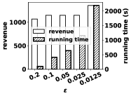
Next, we study the impact of search step on OptPrice, i.e., Algorithm 2. We vary the search step from 0.2, 0.1, 0.05, 0.025 to 0.0125 on all 4 datasets. Besides, we experiment exhaustive search of price on small datasets Residence and Blogs. Note that if the operator iterates all values in as posted price, then he can iterate all possible combination of participating requesters and potential participating suppliers. Thus, exhaustive search of price can be achieved by searching all the values in . However, it is only practical when we only have a finite and small set of requesters. We did not experiment exhaustive price search on the dataset Facebook and DBLP, since it is computationally expensive.
Figure 3 shows the revenue and running time of OptPrice under different selection of search step (including exhaustive search of price) and different budgets on dataset Residence. From Figure 3 one can observe that on the dataset Residence, decreasing the search step can increase the revenue of OptPrice, but it also increases the running time. Moreover, there is a diminishing increase of revenue. We can find that is a proper price search step for the dataset Residence, since it achieves a good balance between running time and performance. The bar labeled as Exh corresponds to exhaustive search of price. On can observe that with a search step , OptPrice can achieve a revenue around 70% of that under exhaustive search of price, which takes at least more than ten times of the running time of OptPrice. Figure 4 shows the results on dataset Blogs. The result is similar to that of the dataset Residence. However, for the dataset Blogs, we can find that is a proper price search step. Figure 5 show the results on dataset Facebook. We can find when we vary search step, the revenues achieved do not change much. Figure 6 shows the results on dataset DBLP. One can observe that 0.05 is a proper search step.


VI Related Work
The notion of social visibility defined in this paper is closely related to social influence [7, 8, 9, 10]. One key difference is that when a user is visible to a set of users, it does not mean this user can influence this set of users. The objective of influence maximization problem is to find a subset of nodes that could maximize the spread of information under certain influence diffusion models. But our problem focuses on the pricing of social visibility service. The idea of adding new links to enhance social visibility is closely related to link prediction [11, 12, 13], and friend recommendation [14, 15, 16, 17], The objectives of link prediction and friend recommendation are to predict future or missing links. Our work adds links that can improve social visibility. Note that such links may have nothing to do with predicting the future or missing links.
Technically, our work is closely related to revenue management [18]. Different with classical revenue management literatures [18], which focuses on understanding the structure of optimal pricing, our work formulates a new revenue maximization framework and we focus design approximation algorithms to solve this problem. Similar to influence maximization [7, 8, 10], the core technique in selecting the supplier set is submodular analysis. Our contribution is in proving that our problem has the submodular property and show that how the submodular property impacts the search optimal pricing.
VII Conclusions
This paper proposes a posted pricing scheme for the OSN operator to price its social visibility boosting service. We formulate a revenue maximization problem for the OSN provider to select the parameter of the posted pricing scheme. We show that the revenue maximization problem is not simpler than an NP-hard problem. We decomposed it into two sub-routines, where one focuses on selecting the optimal set of suppliers, and the other one focuses on selecting the optimal prices. We prove the hardness of each sub-routine, and eventually design a computationally efficient approximation algorithm to solve the revenue maximization problem with provable theoretical guarantee on the revenue gap. We conduct extensive experiments on four public datasets to validate the superior performance of our proposed algorithms.
References
- [1] S. Zheng, H. Xie, and J. C. Lui, Supplementary file to the main paper., 2021. [Online]. Available: https://www.dropbox.com/s/yd0jjtplv97vh41/supplementary.pdf?dl=0
- [2] L. S. Shapley, Notes on the N-person Game–II: The Value of an N-person Game. Rand Corporation, 1951.
- [3] Y. Bachrach, E. Markakis, E. Resnick, A. D. Procaccia, J. S. Rosenschein, and A. Saberi, “Approximating power indices: theoretical and empirical analysis,” Autonomous Agents and Multi-Agent Systems, vol. 20, no. 2, pp. 105–122, 2010.
- [4] J. Kunegis, “KONECT – The Koblenz Network Collection,” in Proc. Int. Conf. on World Wide Web Companion, 2013, pp. 1343–1350.
- [5] J. Leskovec and A. Krevl, “SNAP Datasets: Stanford large network dataset collection,” http://snap.stanford.edu/data, Jun. 2014.
- [6] W. Nawaz, K.-U. Khan, Y.-K. Lee, and S. Lee, “Intra graph clustering using collaborative similarity measure,” Distributed and Parallel Databases, vol. 33, no. 4, pp. 583–603, 2015.
- [7] D. Kempe, J. Kleinberg, and É. Tardos, “Maximizing the spread of influence through a social network,” in Proc. ACM KDD, 2003.
- [8] P. Domingos and M. Richardson, “Mining the network value of customers,” in Proc. ACM KDD. ACM, 2001.
- [9] Y. Lin, W. Chen, and J. C. Lui, “Boosting information spread: An algorithmic approach,” in 2017 IEEE 33rd International Conference on Data Engineering (ICDE). IEEE, 2017, pp. 883–894.
- [10] M. Richardson and P. Domingos, “Mining knowledge-sharing sites for viral marketing,” in Proc. ACM KDD. ACM, 2002.
- [11] L. Lü and T. Zhou, “Link prediction in complex networks: A survey,” Physica A: Statistical Mechanics and its Applications, vol. 390, no. 6, p. 1150–1170, Mar 2011.
- [12] V. Martínez, F. Berzal, and J.-C. Cubero, “A survey of link prediction in complex networks,” ACM CSUR, vol. 49, no. 4, p. 69, 2017.
- [13] D. Liben-Nowell and J. Kleinberg, “The link-prediction problem for social networks,” Journal of the American society for information science and technology, vol. 58, no. 7, pp. 1019–1031, 2007.
- [14] P. Resnick and H. R. Varian, “Recommender systems,” Communications of the ACM, vol. 40, no. 3, pp. 56–59, 1997.
- [15] H. Ma, “On measuring social friend interest similarities in recommender systems,” in Proc. ACM SIGIR. ACM, 2014.
- [16] H. Ma, D. Zhou, C. Liu, M. R. Lyu, and I. King, “Recommender systems with social regularization,” in Proc. WSDM. ACM, 2011.
- [17] X. Xie, “Potential friend recommendation in online social network,” in Proc. IEEE/ACM CGCC. IEEE Computer Society, 2010.
- [18] K. T. Talluri, G. Van Ryzin, and G. Van Ryzin, The theory and practice of revenue management. Springer, 2004, vol. 1.