Prescribed-time Control for Linear Systems in Canonical Form Via Nonlinear Feedback
Abstract
For systems in canonical form with nonvanishing uncertainties/disturbances, this work presents an approach to full state regulation within prescribed time irrespective of initial conditions. By introducing the smooth hyperbolic-tangent-like function, a nonlinear and time-varying state feedback control scheme is constructed, which is further extended to address output feedback based prescribed-time regulation by invoking the prescribed-time observer, all are applicable over the entire operational time zone. As an alternative to full state regulation within user-assignable time interval, the proposed method analytically bridges the divide between linear and nonlinear feedback based prescribed-time control, and is able to achieve asymptotic stability, exponential stability and prescribed-time stability with a unified control structure.
Index Terms:
Nonlinear feedback, prescribed-time stability, output feedback, full state regulationI Introduction
Finite-time convergence is highly desirable in many real-world automation applications, where the ultimate control goals are to be realized within finite time rather than infinite time, e.g., auto parts assembling, spacecraft rendezvous and docking [1, 2], and proportional navigation guidance [3], etc. Various approaches to finite-time convergence have been reported in literature, including: finite-time control, fixed-time control, time-synchronized control, predefined-time control and prescribed-time control. The prototype of the finite-time Lyapunov theory originates from where is a positive definite function, and .
As an effort to achieve finite-time stabilization for high-order systems, the homogeneous method, terminal sliding mode method and adding a power integrator method are successively proposed (see, for instance, [5, 8, 9, 11, 7, 10, 4, 6]), which greatly promote the development of finite-time control theory. Since the convergence (settling) time therein depends on initial conditions and design parameters, the notion of fixed-time control is then introduced in [12] and [13], where the fractional-order plus odd-order feedback is used, leading to different closed-loop system dynamics, so that the upper boundary of the convergence time can be estimated without using initial conditions. However, neither finite-time control nor fixed-time control can actually achieve state regulation within one unified time. The time-synchronized control scheme proposed in [14] and [15], based on the norm-normalized sign function, is shown to be able to achieve output regulation simultaneously for different initial conditions with a unified control law.
To further alleviate the dependence of the settling time on design parameters, a predefined-time approach is exploited to estimate the upper bound of the convergence time in [16] and [17] by multiplying exponential signals on the basis of fractional power feedback signals. Recently, the notion of prescribed-time control is proposed in [18], which allows the user to assign the convergence time at will and irrespective of initial conditions or any other design parameter, thus offers a clear advantage over those that do not. With this concept, three different approaches have been developed, namely, states transformation approach, temporal scale transformation approach, and parametric Lyapunov equation based approach (e.g., [18, 20, 19, 21, 22, 24, 23]). Based on states transformation approach, the distributed consensus control algorithms are studied for multi-agent systems in [25, 27, 26], and a prescribed-time observer based output feedback algorithm is elegantly established for linear systems in [28]. Subsequent works further consider more complex systems, such as stochastic nonlinear systems [29] and LTI systems with input delay [30]. In addition, by using temporal scale transformation, a triangularly stable controller is proposed for the perturbed system in [31], a dynamic high-gain feedback algorithm is established for strict-feedback-like systems in [19], and some distributed algorithms are developed for multi-agent systems in [32, 33, 34]. Based upon parametric Lyapunov equation, a finite-time controller and a prescribed-time controller are studied for linear systems in [1] and [21], and then generalized to nonlinear systems in [35].
Theoretically inclined, prescribed-time control systems, under some generic design conditions, are capable of tolerating large parametric, structural and parameterizable disturbance uncertainties on the finite time interval, to ensure desired control performance, in addition to system stability. This property comes from a time-varying function which goes to as tends to the prescribed time. Different from [18, 25, 22], where the time-varying function is used to scale the coordinate transformations, this paper only introduces the time-varying function into the virtual/actual controller. The advantage of this approach is that a simpler controller results and the control effort is reduced. In addition, to obtain far superior transient performance, we choose a new feedback scheme that the regular feedback signal can be reconstructed into some suitable forms by a nonlinear mechanism with high design degrees of freedom.111Some early literature exploit similar ideas to improved control performance. For example, in classical proportional-integral-differential (PID) control, the feedback signal is processed by proportion, integral or differential to construct the classical PI, PD or PID control.
Motivated by the above discussions, this paper revisits the prescribed-time control of high-order systems via a novel nonlinear feedback approach. In Section II, a useful hyperbolic-tangent-like function and a novel lemma are presented. In Section III, we study the prescribed-time control for certain LTI systems by using a nonlinear and time-varying feedback, both full state feedback and partial state feedback are considered. Section IV gives a extend prescribed-time control algorithm for uncertain LTI systems. Section V concludes this paper. The main contributions of this paper are as follows:
-
•
Both full state and partial state feedback controller are designed to achieve state regulation within prescribed time irrespective of initial conditions and any other design parameter. A non-stop running implementation method with ISS property is proposed for the first time.
-
•
Unlike most existing solutions that usually use the regular (direct) state feedback, this paper proposes to use the “reshaped” feedback states through the hyperbolic-tangent-like function, so as to establish a nonlinear and time-varying feedback control strategy capable of addressing asymptotic, exponential and prescribed-time control uniformly under certain conditions.
-
•
For high-order systems with non-parametric uncertainties/disturbances, we propose a prescribed-time sliding mode control scheme, melting attractive stability and robustness features at the transition and steady-state stages.
Notations: is the set of nonnegative real numbers, . For non zero integers and , let be the -matrix with zero entries, and and where . denotes on . Denote by the set of class -functions and denote by the set of class -functions (see Section 4.4 in [37]). For any vector , we use and to denote its transpose and Euclidean norm respectively. denotes the limit of as . We denote by the -th derivative of , and denote by the -th power of .
II Preliminaries
II-A Problem Statement
We restrict our analysis to the following system in canonical form with uncertainties/disturbances
| (1) |
where is the system matrix, , are coefficient vectors, with modeling the unknown nonvanishing uncertainties/disturbances of the system, is the vector of system states, and is the control input. is controllable and is observable. The control objective is to design a feedback control to stabilize (1) within prescribed-time , i.e., and We are particularly interested in making use of the feedback information through a nonlinear way to construct the control scheme.
Definition 1
[30] The origin of the system is said to be prescribed-time globally asymptotically stable (PT-GUAS) if there exist a class function and a function such that tends to infinity as goes to and,
where is a time that can be prescribed in the design.
II-B Hyperbolic-tangent-like Function
Instead of using directly, we process the feedback information through the following hyperbolic-tangent-like function as:
| (2) |
where and are design parameters, which becomes the standard hyperbolic tangent function for . Such nonlinear feedback exhibits two salient properties.
Property 1: The function is on and if and only if . Under , the inequality holds.
Proof: Define a continuous function . For , we have
For , it follows that
Thus, under , the inequality holds for , implying that for .
Property 2: Function is strictly monotonically increasing with respect to (w.r.t.) , its upper and lower bounds are and , respectively. By selecting different design parameters and , various functions can be obtained from , In particular, if choosing and small enough, then .
Proof: The upper and lower bounds of are
When and are sufficiently small, for , by using L’Hpital’s Rule, we have
implying that the expanded/compressed signal reverses back to the regular signal .
Remark 1
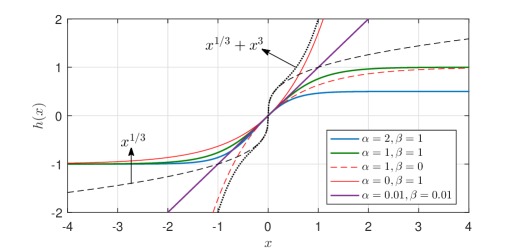
The classical finite-time control adopts fractional power of (i.e., ) to expand the feedback signal on , and compress on ; the fixed-time control uses an additional nonlinear damping term on the basis of the original feedback signal to expand the feedback signal on . Consequentially, different feedback signals cause different convergence properties, which is mainly reflected in the relationship between settling time and initial conditions. Since the hyperbolic-tangent-like function can expand or compress the feedback signal with different and , it provides control design extra flexibility and degree of freedom. In addition, the right-hand side of (2) remains bounded within even if grows large, this special property makes perfectly suitable to function as the core part of the controller, and our motivation for this work partly stems from such appealing features of . Fig. 1 illustrates with different and , and the fractional power feedback signals in terms of .
The interesting feature behind this nonlinear feedback is that it includes regular (direct) feedback of as a special case, and it allows the linear regular feedback control and nonlinear feedback control to be unified through such function, providing a variety of ways to making use of for control development. By using properties of the hyperbolic-tangent-like function, we establish the following lemma, which is crucial to our later technical development.
Lemma 1
Consider the functions and be given as in (2). For , if a positive continuously differentiable function satisfies
| (3) |
where if and only if , then we have and being of class-. In particular, it holds
Proof: Consider the analytical expression of (3):
| (4) |
Let , where . Then we have , and
| (5) | ||||
holds for . Hence we derive according to Lemma 1 in [18], namely and . The same result can be established for . It follows from the fact tends to “slower” than as that and . In addition, the inequality (4) can be transformed into the following form:
| (6) |
where is the integral constant. In fact, one can easily verify the following calculations
Furthermore, from (6.3) we have and
| (7) |
Indeed, notice that is a continuous function and for , implying that and as . This completes the proof.
As discussed earlier, when and are sufficiently small, we have . Lemma 1 is therefore equivalent to the Corollary 1 in [18].
III Prescribed-time control for linear systems in canonical form without uncertainties
Motivated by the appealing features of the nonlinear scaling function , we now discuss how to introduce it into the prescribed-time control design of -th order systems (1). We first design prescribed-time control schemes using nonlinear and time-varying full state feedback and partial state feedback to achieve full state regulation for system (1) without uncertainties/disturbances (i.e., ), then we extend the control scheme to cope with nonvanishing uncertainties/disturbances in the system.
III-A Prescribed-time State Feedback Controller
By using the time-varying scaling function and the hyperbolic-tangent-like function as introduced in Section 2, we construct the vectors as
| (8) | ||||
where and is defined in (2). In addition, we introduce the following two auxiliary vectors
| (9) | ||||
where , . Note that is lower triangular, thus both and can be easily calculated recursively (see (28) for specific example of computing and ). It is interesting to see that the convergence property of the closed-loop system only depends on the parameters , , and in vector .
Theorem 1
Consider system (1) with and the state feedback control law,
| (10) |
then all closed-loop signals are bounded and the origin of the closed-loop system (1) is:
-
Globally uniformly asymptotically stable (GUAS), that is, , if the controller parameters are selected as and . In addition, exponential output regulation is achieved if and are chosen sufficiently small.
-
Prescribed-time globally uniformly asymptotically stable (PT-GUAS), that is, , if the controller parameters are selected as and .
Proof: By the definition of , and , it is readily verified that and , therefore, it holds that
| (11) | ||||
1) proof of GUAS result: we prove that the closed-loop system under the control law (10) with (in this case, ) is GUAS. To this end, we define the error vector between and as
| (12) |
where is a smooth function satisfying and is bounded as long as is bounded. Consider a positive definite function , the time derivative of along (11) is
| (13) |
where the fact that is used since is a skew symmetric matrix. It follows from (13) that if and only if , thus the transformed system (11) is asymptotically stable on , establishing the same to system (1) according to the converging-input converging-output property of the corresponding auxiliary vectors.
From (13), it can be further shown that
| (14) | ||||
where . By integrating both sides of the inequality (14), we obtain . If we further choose the design parameters and in small enough, one can obtain , yielding , thus we have and the transformed system (11) is exponentially stable. In addition, it follows from (9) that , therefore exponential output regulation to zero of (1) can be achieved. The word “exponential” actually means that “near exponential”, because the parameters and can only be selected as sufficiently small, not zero.
2) Proof of PT-GUAS result: we now show that the closed-loop system under the control law (10) with (in this case, ) is PT-GUAS. For there exists a continuous positive function such that as and
| (15) |
In addition, its time derivative can be shown as
| (16) | ||||
Using Property 1 and (15), we have
| (17) | ||||
Since we select , then . By virtue of Lemma 1, one can prove that , and
| (18) |
Hence the closed-loop signals and , and meanwhile converge to zero as tends to . Using the property of the hyperbolic-tangent-like function, we can proceed to prove that and the convergence of which to zero at the prescribed time.
By means of the auxiliary vectors as introduced in (9), one can find that and the following closed-loop -dynamics holds
| (19) |
where is a bounded function, which also can be treated as a vanishing disturbance. When , the equivalent form of (19) is
| (20) |
It follows from (4)-(6) and (20) that
| (21) |
where . Then taking time derivative on both sides of (21), we have
| (22) |
Observe that (22) means that as . Continue, using the analysis similar to that used in (21)-(22), by taking the -th derivative of both sides of (21), we can generalize that and converge to zero as (this is the reason for ). Therefore, and hold.
In addition, it follows from (9) that , therefore , then
| (23) |
Consequently, from (10) we have
| (24) | ||||
Note that each term in the third line of (24) is bounded on and converges to zero as . Therefore, and This completes the proof.
Remark 2
When we consider a scalar system , from Theorem 1, one can immediately obtain a prescribed-time controller as . Note that according to Theorem 1, this controller is only a special case under the design parameters and are chosen as small enough, and the design parameter satisfies . Note that the classical finite-time controllers (see [4, 21]), then the unique dynamic solution is
where . Thereafter, the finite-time controller is equivalent to
| (25) | ||||
Inserting into (25), we have
| (26) | ||||
Let , we have . The above analysis proves that the prescribed-time controller is equivalent to the finite-time controller under choosing some special design parameters.
Remark 3
If we utilize the PT-GUAS controller (as defined in (10) with ) and the GUAS controller () through the following way,
then the system states converge to zero as and then remain zero for . In fact, this switching method means that the prescribed-time controller guarantees that the closed-loop system is PT-GUAS on and the GUAS controller guarantees that the closed-loop system is ISS in the presence of some external disturbance on .
Remark 4
Various methods on finite-time control have been reported in literature during the past few years, among which the most typical ones include adding a power integral (AAPI), linear matrix inequalities (LMI) and implicit Lyapunov function (ILF), where the key element utilized is the fractional power state feedback (e.g., [10, 12, 11]). In pursuit of an alternative solution, we exploit a unified control law such that the closed-loop system (11) can be regulated asymptotically, exponentially or within prescribed-time by choosing the design parameters , and in (12) properly. One salient feature with this method is that it analytically bridges the divide between prescribed-time control and traditional asymptotic control. Furthermore, different design parameters ( and in ) allow different reshaped feedback signals to be utilized in the control scheme. Such treatment provides extra design flexibility and degree of freedom in tuning regulation performance.
Remark 5
Compared with the existing prescribed-time control results (see, for instance, [18, 38, 28, 22]), the proposed NTV feedback scheme, making use of the reshaped (compressed/expanded) feedback signal, is applicable over the entire operational process. In addition, this scheme has a numerical advantage over the aforementioned methods, this is because here only rather than is involved for state scaling. Furthermore, with the proposed hyperbolic tangent function, the magnitude of initial control input can be adjusted through the parameters and .
Example 1
To verify the effectiveness and benefits of control scheme as presented Theorem 1, we conduct a comparative simulation study through a third-order system
According to Theorem 1-GUAS, the asymptotically stabilization controller under is with and the control parameters are selected as , ; and the initial condition are selected as . According to Theorem 1-PT-GUAS, the following NTV feedback prescribed-time stabilization controller can be obtained,
| (27) |
with
| (28) | ||||
where the corresponding design parameters are selected as , , . In addition, to compare the control performance, we adopt our previous result (a linear feedback scheme in [18]) for simulation, the corresponding control law is given by , where , , . The design parameters in are selected as , and .
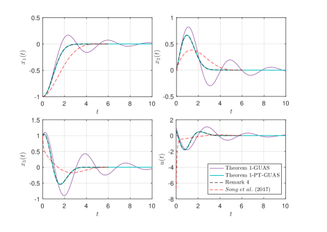
For comparison, simulation results obtained with the three different control schemes are shown in Fig. 2, from which asymptotic stabilization and prescribed-time stabilization are observed. Furthermore, it is seen that the settling time with the proposed prescribed-time control is indeed irrespective of initial condition and any other design parameter; the proposed scheme works within and after the prescribed-time interval; and compared with linear feedback scheme (black dotted line), it can be seen that the NTV feedback schemes (red dotted line and blue solid line) have a superior transient performance with a smaller initial control effort, verifying the effectiveness and benefits of the proposed algorithms.222Our design is another option in the control designer’s toolbox and we do not claim its universality with respect to the existing designs but highlight its better control performance of a class of LTI systems.
III-B Prescribed-time Observer
When only partial state is measurable, we employ the prescribed-time observer proposed in [38], to construct the prescribed-time control using output feedback. As in [38] and [36], our solution is based on the separation principle, namely the controller is derived by designing a prescribed-time observer and a NTV output feedback control separately.
Considering that and only output is available for feedback. The system (1) can be transformed into the following observer canonical form by a linear nonsingular transformation
| (29) |
where , , , and the s, s are the same as those in (1).
Invoking the observer proposed in [38], as follows
| (30) | ||||
where the time-varying observer gains satisfy
where and
| (31) | ||||
and is an integer and is selected to make the -dimensional matrix Hurwitz. With (29)-(30) and observer error state , we get the observer error dynamics
| (32) |
Lemma 2
[38] For the dynamic system (1), consider the observer (30) having error dynamic (32) and observer gains , and the are constants to be selected such that the companion matrix is Hurwitz, then the closed-loop observer error system (32) is prescribed-time stable, and there exist two positive constants and such that
| (33) |
for all . In addition, the output estimation error injection terms remain uniformly bounded over , and converge to zero as Also, has the same dynamic properties as since with being a nonsingular constant matrix.
III-C Prescribed-time Output Feedback Controller
The output feedback prescribed-time control law for system (1) is constructed by replacing with in (10) as follows:
| (34) |
where only is measurable, with and
The control law (34) involves the design parameters and as defined in Theorem 1. It can be verified that different and lead to different convergence rate. For instance, we can set and , and by invoking the classical high-gain observer, to achieve asymptotic or exponential output regulation. Here in this subsection, our ambitious goal is to achieve state regulation with output feedback with the aid of the prescribed-time observer developed in [38].
Theorem 2
Proof: The proof consists of two steps, the first step is to prove that the closed-loop system with the observer and the output feedback control scheme does not escape during , and the second step is to show that all closed-loop trajectories converge to zero as tends to and remain zero thereafter.
Step 1: We consider the Lyapunov function . Using and , the derivative of over along (1) under the output feedback control law (34) becomes
where , . It is seen from Lemma 2 that remains uniformly bounded over and converges to zero as . The boundedness of is also guaranteed by the bounded , and also converges to zero as tends to . Therefore, there exist a positive constant such that holds for . It follows that and cannot escape during the interval
Step 2: From Lemma 2, we know that there exists a prescribed-time , such that for . In consequence, the output feedback control law coincides with state feedback control law for . In other words, this output feedback law can be used to establish prescribed-time stability and performance recovery (see [37, 36] and [28]). Note that the closed-loop trajectory under (34) does not escape during , it follows from Theorem 1-PT-GUAS that under the proposed output feedback control law, there exists another pre-set time to steer the system from an arbitrary bounded state to zero as The boundedness of can also be easy established according to Theorem 1. This completes the proof.
Remark 6
To close this section, it is worth making the following comments.
-
The output feedback controller inherits the properties and advantages of the state feedback controller as stated in Theorem 1, that is, elegant parameter tuning, one-step design process, simple controller structure.
-
Prescribed-time stabilization is the result of employing the scaling function and the nonlinear feedback function inside the control scheme (10). All observer errors are regulated to zero within the pre-set time , and all system states are regulated to zero within pre-set time , where .
-
Only the output state is required in constructing the output feedback prescribed-time control (34). Such control scheme has an obvious numerical advantage because its maximum implemented gain is , while the standard linear -th order output feedback prescribed-time controller proposed in [28] involves .
-
It is noted that the time-varying gains , go to infinity as time tends to or , such phenomenon (unbounded control gain at the fixed convergence time) appears in all results on strictly finite-/fixed-/prescribed-time control. The implementation solution for finite-/fixed-time control is to use fractional power state feedback or sign functions switching the controller to zero when the system is regulated to the equilibrium point. The other implementation solutions for prescribed-time control are given in [28, 20, 18]. One typical way to address this issue is to let the system operate in a finite-time interval, i.e., adjusting the operational time slightly shorter than prescribed convergence time. Another typical way is to let the system operate in an infinite time interval by making suitable saturation on the control gains. Here in this work, we use the method as described in Remark 3 to implement the prescribed-time controller for and initiate the asymptotically stable controller for .
Example 2
We illustrate the performance of the observer and the output feedback controller through the following model:
the observer is
| (35) |
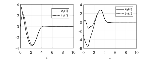
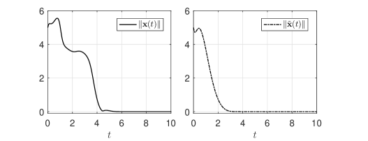
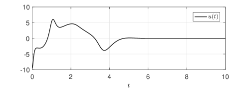
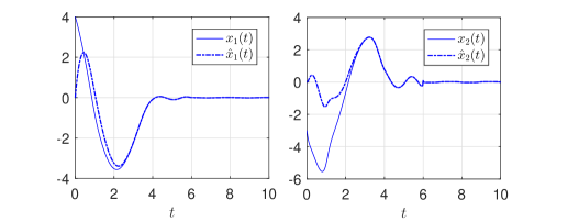
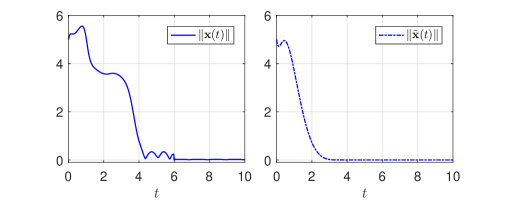
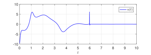
with , . For observer parameters, we select , , s and . For output feedback controller parameters, we select , and s. The initial condition is . The control law is implemented similar to (28), just replacing in (28) with . Furthermore, the control performance in a noisy environment is studied by considering the output signal corrupted with an uncertain measurement noise , namely with . The closed-loop state trajectories, state estimate trajectories, the norm of observer estimation error , the norm of system state and control input signal are shown in Figs. 3-4.
It is observed from Fig. 3 that the controller remains operational after , and all closed-loop signals are bounded on the whole time-domain, in particular, the observer estimation errors converge to zero as , and system states converge to zero as , confirming our theoretical prediction and analysis. Fig. 4 shows that the proposed controller retains its performance even in the presence of measurement noise. Although a slightly chattering phenomenon, caused by noise and controller switching, occurs near , the control input remains bounded on the whole time-domain. In addition, the numerical advantage leading to friendly implementation has been verified in simulation.
IV Prescribed-time control for linear systems in canonical form with uncertainties
In the presence of non-vanishing uncertain term , system (1) can be rewritten as
| (36) |
where is an unknown smooth function and satisfies with being a known scalar real-valued function.
Define a sliding surface on as follows:
| (37) |
where is defined in (9). Some other sliding surface selection can be referred to [39] and [40]. The derivative of the auxiliary variable along the trajectories of (36) is
| (38) |
where belongs to a computable function.
Theorem 3
Consider system (1) and the transformed system (36), the closed-loop signals and are prescribed-time globally uniformly asymptotically stable (PT-GUAS), if the control law is designed as:
| (39) |
where , , , is a computable function as described after (38), and is the hyperbolic-tangent-like function as defined in (2).
Proof: For , let . With the control scheme (39), for , the upper right-hand derivative of along the trajectory of the closed-loop system (36) becomes
| (40) |
By using Lemma 1, it is easy to get that and , establishing the same for and . At the same time, the closed-loop -dynamics become
| (41) | ||||
where is the virtual control input. It is seen that the control law (39) reduces the perturbed -th order system to an unperturbed -th order system. Therefore, by using Theorem 1-PT-GUAS, we can prove that the closed-loop signals , , and are bounded and converge to zero as . From (40) and the analysis process in Section 3, it is not difficult to verify that is also bounded. Therefore, it follows from (39) that the control input is bounded for . This completes the proof.
Remark 7
For , we specifically design as , where are assigned such that the polynomial is Hurwitz, and design the corresponding control law as . As a result, , we therefore obtain that by recalling that . Furthermore, it is not difficult to get . As the disturbances do not disappear, the control action for is no longer zero but bounded, a necessary effort to fight against the ever-lasting (nonvanishing) uncertainties/disturbances, which is comprehensible in order to maintain each state at the equilibrium (zero) after the prescribed settling time.
Example 3
To verify the effectiveness of the prescribed-time sliding mode controller, we consider the following system:
where
| (42) |
here can be selected as . According to Theorem 3, the controller is given by
| (43) |
with
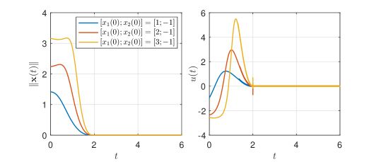
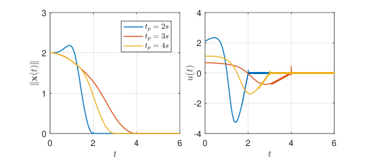
In addition, according to Remark 6, we design with . For simulation, the design parameters are chosen as and . To verify the property of prescribed-time convergence w.r.t. the initial conditions, three different initial values , and are considered in Fig. 5. To confirm the property of prescribed-time convergence w.r.t. , we choose respectively in Fig. 6.
Simulation results show that: all states converge to zero synchronously within the pre-set time ; and the convergence time is independent of initial conditions and any other design parameter. Certain control chattering is observed as , which is caused by the auxiliary variable and controller switching. Specially, the magnitude of control input has a slight increase when increases or decreases.
V Conclusions
A unified nonlinear and time-varying feedback control scheme is developed to achieve prescribed-time regulation of high-order uncertain systems. The proposed control is able to achieve asymptotic, exponential, or prescribed-time regulation by selecting the design parameters properly. The rule of parameter selection has been given through the Lyapunov theory. Furthermore, prescribed-time output feedback control and prescribed-time sliding mode control for high-order systems are developed, where the advantages of simplicity (elegancy) yet superiority are retained. Extension of the proposed method to more general nonlinear systems with mismatched uncertainties represents an interesting future research topic.
References
- [1] B. Zhou, “Finite-time stabilization of linear systems by bounded linear time-varying feedback,” Automatica, vol. 113, pp. 108760, Nov. 2020.
- [2] L. Zhao, J. P. Yu, and P. Shi, “Command Filtered Backstepping-Based Attitude Containment Control for Spacecraft Formation,” IEEE Trans. Syst., Man, Cybern. Syst., vol. 51, no. 2, pp. 1278-1287, Feb. 2021.
- [3] P. Zarchan, Tactical and strategic missile guidance (6th ed.). AIAA. 2012.
- [4] S. P. Bhat, and D. S. Bernstein, “Continuous finite-time stabilization of the translational and rotational double integrators,” IEEE Trans. Autom. Control, vol. 43, no. 5, pp. 678-682, May. 1998.
- [5] S. P. Bhat, and D. S. Bernstein, “Geometric homogeneity with applications to finite-time stability,” Math. Control Signal Syst., vol. 17, no. 2, pp. 101-127, May. 2005.
- [6] L. Zhao, J. P. Yu, C. Lin, and Y. M. Ma, “Adaptive Neural Consensus Tracking for Nonlinear Multiagent Systems Using Finite-Time Command Filtered Backstepping,” IEEE Trans. Syst., Man, Cybern. Syst., vol.48, no. 11, pp. 2003-2018, Nov. 2018.
- [7] M. Chen, Q. X. Wu, and R. X. Cui, “Terminal sliding mode tracking control for a class of SISO uncertain nonlinear systems,” ISA Trans., vol. 52, no. 2, pp. 198-206, Nov. 2013.
- [8] A. Levant, “Higher-order sliding modes, differentiation and output-feedback control,” Int. J. Control, vol. 76, no. 9, pp. 924-941, Sep. 2003.
- [9] A. Levant, “Homogeneity approach to high-order sliding mode design,” Automatica, vol. 41, no. 5, pp. 823-830, May. 2005.
- [10] F. Amato, M. Ariola, and P. Dorato, “Finite-time control of linear systems subject to parametric uncertainties and disturbances,” Automatica, vol. 37, no. 9, pp. 1459-1463, Sep. 2001.
- [11] W. Lin, and C. J. Qian, “Adding a power integrator: a tool for global stabilization of high-order lower-triangular systems,” Syst. and Control Lett., vol. 39, no. 5, pp. 339-351, Apr. 2000.
- [12] A. Polyakov, D. Efimov, and W. Perruquetti, “Finite-time and fixed-time stabilization: implicit lyapunov function approach,” Automatica, vol. 51, pp. 332-340, Jan. 2015.
- [13] A. Polyakov, “Nonlinear feedback design for fixed-time stabilization of linear control systems,” IEEE Trans. Autom. Control, vol. 57, no. 8, pp. 2106-2110. Aug. 2012.
- [14] D. Y. Li, S. S. Ge, and T. H. Lee, “Fixed-time-synchronized consensus control of multi-agent systems,” IEEE Trans. Control Netw. Syst., vol. 8, no. 1, pp. 89-98, Mar. 2021.
- [15] D. Y. Li, H. Y. Yu, K. P. Tee, Y. Wu, S. S. Ge, and T. H. Lee, “On time-synchronized stability and control,” IEEE Trans. Syst. Man Cybern. Syst., pp. 1-14. Jan. 2021.
- [16] J. D. Sánchez-Torres, E. N. Sanchez, and A. G. Loukianov, “Predefined time stability of dynamical systems with sliding modes,” in Proc. Amer. Control Conf., 2015, pp. 5842–5846.
- [17] J. D. Sánchez-Torres, D. Gómez-Gutierrez, E. López, and A. G. Loukianov, “A class of predefined-time stable dynamical systems,” IMA J. Math. Control Inf., vol. 35, no. 1, pp. 1-29, Apr. 2018.
- [18] Y. D. Song, Y. J. Wang, J. Holloway, and M. Krstić, “Time-varying feedback for regulation of normal-form nonlinear systems in prescribed finite time,” Automatica, vol. 83, pp. 243-251, Sep. 2017.
- [19] P. Krishnamurthy, F. Khorrami, and M. Krstić, “Robust adaptive prescribed-time stabilization via output feedback for uncertain nonlinear strict-feedback-like systems,” Eur. J. Control, vol. 55, pp. 14-23, Sep. 2019.
- [20] P. Krishnamurthy, F. Khorrami, and M. Krstić, “A dynamic high-gain design for prescribed-time regulation of nonlinear systems,” Automatica, vol. 115, pp. 108860, May. 2020.
- [21] B. Zhou, “Finite-time stability analysis and stabilization by bounded linear time-varying feedback,” Automatica, vol. 121, pp. 109191, Nov. 2020.
- [22] Y. D. Song, Y. J. Wang, and M. Krstić, “Time-varying feedback for stabilization in prescribed finite time,” Int. J. Robust and Nonlinear Control, vol. 29, no. 3, pp. 618-633. Mar. 2019.
- [23] H. F. Ye, and Y. D. Song, “Prescribed‐time control of uncertain strict‐feedback‐like systems,” Int. J. Robust and Nonlinear Control, vol. 31, pp. 5281-5297, Mar. 2021.
- [24] Z. Kan, T. Yucelen, E. Doucette, and E. Pasiliao, “A finite-time consensus framework over time-varying graph topologies with temporal constraints,” J. Dyn. Syst. Meas. Control, vol. 139, no. 7, pp. 1-6, Jul. 2017.
- [25] Y. J. Wang, and Y. D. Song, “Leader-following control of high-order multi-agent systems under directed graphs: Pre-specified finite time approach,” Automatica, vol. 87, pp. 113-120, Jan, 2018.
- [26] Y. J. Wang, Y. D. Song, and D. J. Hill, “Zero-error consensus tracking with preassignable convergence for nonaffine multiagent systems,” IEEE Trans. Cybern., vol. 51, no. 3, pp. 1300-1310, Mar. 2021.
- [27] Y. J. Wang, Y. D. Song, D. J. Hill, and M. Krstić, “Prescribed-Time Consensus and Containment Control of Networked Multiagent Systems,” IEEE Trans. Cybern., vol. 49, no. 4, pp. 1138-1147, Apr. 2019.
- [28] J. Holloway, and M. Krstić, “Presribed-time output feedback for linear systems in controllable canical form,” Automatica, vol. 107, pp. 77-85, May. 2019.
- [29] W. Li, and M. Krstić, “Stochastic nonlinear prescribed-time stabilization and inverse optimality,” IEEE Trans. Autom. Control, in press, 2021.
- [30] N. Espitia, and W. Perruquetti, “Predictor-feedback prescribed-time stabilization of LTI systems with input delay,” IEEE Trans. Autom. Control, in press. 2021.
- [31] A. Shakouri, and N. Assadian, “Prescribed-time control with linear decay for nonlinear systems,” IEEE Control Syst. Lett., in press. 2021.
- [32] T. Yucelen, Z. Kan, and E. Pasiliao, “Finite-Time Cooperative Engagement,” IEEE Trans. Autom. Control, vol. 64, no. 8, pp. 3521-3526, Aug. 2019.
- [33] D. Tran, and T. Yucelen, “Finite-time control of perturbed dynamical systems based on a generalized time transformation approach,” Syst. and Control Lett., vol. 136, pp. 104605, Feb. 2020.
- [34] E. Arabi, and T. Yucelen, “Control of Uncertain Multiagent Systems with Spatiotemporal Constraints,” IEEE Trans. Control Netw. Syst., vol. 8, no. 3, pp. 1107-1115, Sep. 2021.
- [35] B. Zhou, and Y. Shi, “Prescribed-time stabilization of a class of nonlinear systems by linear time-varying feedback,” IEEE Trans. Autom. Control, in press, 2021.
- [36] B. L. Tian, Z. Y. Zuo, X. M. Yan, and H. Wang, “A fixed-time output feedback control scheme for double integrator systems,” Automatica, vol. 80, pp. 17-24, Jun, 2017.
- [37] H. K. Khalil, Nonlinear systems (3rd ed.), Englewood Cliffs, USA: Prentice-Hall. 2002.
- [38] J. Holloway, and M. Krstić, “Prescribed-Time observers for linear systems in observer canonical form,” IEEE Trans. Autom. Control, vol. 64, no. 9, pp. 3905-3912, Sep. 2019.
- [39] N. Harl, and S. N. Balakrishnan, “Impact Time and Angle Guidance With Sliding Mode Control,” IEEE Trans. Control Syst. Technol., vol. 20, no. 6, pp. 1436-1449, Nov. 2012.
- [40] Z. R. Chen, X. Ju, Z. W. Wang, and Q. Li, “The prescribed time sliding mode control for attitude tracking of spacecraft,” Asian Journal of Control, Apr. 2020.