Preferential Bayesian optimisation with Skew Gaussian Processes
Abstract
Bayesian optimisation (BO) is a very effective approach for sequential black-box optimization where direct queries of the objective function are expensive. However, there are cases where the objective function can only be accessed via preference judgments, such as "this is better than that" between two candidate solutions (like in A/B tests or recommender systems). The state-of-the-art approach to Preferential Bayesian Optimization (PBO) uses a Gaussian process to model the preference function and a Bernoulli likelihood to model the observed pairwise comparisons. Laplace’s method is then employed to compute posterior inferences and, in particular, to build an appropriate acquisition function. In this paper, we prove that the true posterior distribution of the preference function is a Skew Gaussian Process (SkewGP), with highly skewed pairwise marginals and, thus, show that Laplace’s method usually provides a very poor approximation. We then derive an efficient method to compute the exact SkewGP posterior and use it as surrogate model for PBO employing standard acquisition functions (Upper Credible Bound, etc.). We illustrate the benefits of our exact PBO-SkewGP in a variety of experiments, by showing that it consistently outperforms PBO based on Laplace’s approximation both in terms of convergence speed and computational time. We also show that our framework can be extended to deal with mixed preferential-categorical BO, typical for instance in smart manufacturing, where binary judgments (valid or non-valid) together with preference judgments are available.
1 Introduction
Bayesian optimization (BO) is a powerful tool for global optimisation of expensive-to-evaluate black-box objective functions (Brochu et al.,, 2010; Mockus,, 2012). However, in many realistic scenarios, the objective function to be optimized cannot be easily quantified. This happens for instance in optimizing chemical and manufacturing processes, in cases where judging the quality of the final product can be a difficult and costly task, or simply in situations where only human preferences are available, like in A/B tests (Siroker and Koomen,, 2013). In such situations, Preferential Bayesian optimization (PBO) (González et al.,, 2017) or more general algorithms for active preference learning should be adopted (Brochu et al.,, 2008; Zoghi et al.,, 2014; Sadigh et al.,, 2017; Bemporad and Piga,, 2019). These approaches require the users to simply compare the final outcomes of two different experiments and indicate which they prefer. Indeed, it is well known that humans are better at comparing two options rather than assessing the value of “goodness” of an option (Thurstone,, 1927; Chernev et al.,, 2015).
This contribution is focused on PBO. As in state-of-the-art approach for PBO (González et al.,, 2017), we use a Gaussian process (GP) as a prior distribution of the latent preference function and a probit likelihood to model the observed pairwise comparisons. However, our contribution differs from and improves González et al., (2017) in several directions.
First, the state-of-the-art PBO methods usually approximate the posterior distribution of the preference function via Laplace’s approach. On the other hand, we compute the exact posterior distribution, which we prove to be a Skew Gaussian Process (SkewGP) (recently introduced in Benavoli et al., (2020) for binary classification).111In particular, the present works extends the results in Benavoli et al., (2020) by showing that SkewGPs are conjugate to probit affine likelihoods. This allows us to apply SkewGPs for preference learning. Through several examples, we show that the posterior has a strong skewness, and thus any approximation of the posterior that relies on a symmetric distribution (such as Laplace’s approximation) results in sub-optimal predictive performances and, thus, slower convergence in PBO.
Second, we propose computationally efficient methods to draw samples from the posterior that are then used to calculate the acquisition function.
Third, we extend standard acquisition functions used in BO to deal with preference observations and propose a new acquisition function for PBO obtained by combining the dueling information gain with the expected probability of improvement.
Fourth, we define an affine probit likelihood to model the observations. Such a likelihood allows us to handle, in a unified framework, mixed categorical and preference observations. These two different types of information are usually available in manufacturing, where some parameters may cause the process to fail and, therefore, producing no output. In standard BO, where the function evaluation is a scalar, a common way to address this problem is by penalizing the objective function when no output is produced, but this approach is not suitable in PBO as the output is not a scalar.
The rest of the paper is organized as follows. A review on skew-normal distributions and SkewGP is provided in Section 2. The main results of the paper are reported in Section 3, where we show that the posterior distribution of the latent preference function is a SkewGP under the proposed affine probit likelihood. The marginal likelihood is derived and maximized to chose the model’s hyper-parameters. An illustrative example is presented in 4 to show the drawbacks of Laplace’s approximation, thus highlighting the benefits of computing the exact SkewGP posterior distribution. PBO through SkewGP is discussed in Section 5, where extensive tests with different acquisition functions are reported and clearly show that PBO based on SkewGP consistently outperforms Laplace’s approximation both in terms of convergence speed and computational time.
2 Background on skew-normal distributions and skew-Gaussian processes
In this section we provide details on the skew-normal distribution. The skew-normal (O’Hagan and Leonard,, 1976; Azzalini,, 2013) is a large class of probability distributions that generalize a normal by allowing for non-zero skewness. A univariate skew-normal distribution is defined by three parameters location , scale and skew parameter and has the following (O’Hagan and Leonard,, 1976) Probability Density Function (PDF)
where and are the PDF and Cumulative Distribution Function (CDF), respectively, of the standard univariate Normal distribution. Over the years many generalisations of this distribution were proposed, in particular Arellano and Azzalini, (2006) provided a unification of those generalizations in a single and tractable multivariate Unified Skew-Normal distribution. This distribution satisfies closure properties for marginals and conditionals and allows more flexibility due the introduction of additional parameters.
2.1 Unified Skew-Normal distribution
A vector is distributed as a multivariate Unified Skew-Normal distribution with latent skewness dimension , , if its probability density function (Azzalini,, 2013, Ch.7) is:
| (1) |
where represents the PDF of a multivariate Normal distribution with mean and covariance , with being a correlation matrix and a diagonal matrix containing the square root of the diagonal elements in . The notation denotes the CDF of evaluated at . The parameters of the SUN distribution are related to a latent variable that controls the skewness, in particular is called Skewness matrix.
 |
 |
| (a1) , | (a2) , |
 |
 |
 |
 |
| (a1) , | (a2) , | (a3) , | (a4) , |
| , |
The PDF (1) is well-defined provided that the matrix
| (2) |
i.e., is positive definite. Note that when , (1) reduces to , i.e. a skew-normal with zero skewness matrix is a normal distribution. Moreover we assume that , so that, for , (1) becomes a multivariate Normal distribution.
Figure 1 shows the density of a univariate SUN distribution with latent dimensions (a1) and (a2). The effect of a higher latent dimension can be better observed in bivariate SUN densities as shown in Figure 2. The contours of the corresponding bivariate normal are dashed. We also plot the skewness directions given by .
For what follows however it is important to know that (see, e.g., Azzalini,, 2013, Ch.7) the distribution is closed under marginalization and conditioning. We have reviewed these results in Appendix A together with an additive representation of the SUN that is useful for sampling from the posterior.
A SkewGP Benavoli et al., (2020) is a generalization of a skew-normal distribution to a stochastic process. Its construction is based on a result derived by Durante, (2019) for the parametric case, who showed that the skew-normal distribution and probit likelihood are conjugate.
To define a SkewGP, we consider here a location function , a scale (kernel) function , a skewness vector function and the parameters . A real function is a SkewGP with latent dimension , if for any sequence of points , the vector is skew-normal distributed with parameters and location, scale and skewness matrices, respectively, given by
| (3) |
The skew-normal distribution is well defined if the matrix is positive definite for all and for any . In that case we write . Benavoli et al., (2020) shows that this is a well defined stochastic process. In the next section we connect this stochastic process to preference learning.
3 SkewGP and affine probit likelihood
Consider input points , with , and a data-dependent matrix . We define an affine probit likelihood as
| (4) |
where is the standard -variate Gaussian CDF evaluated at with identity covariance matrix. Note that this likelihood model includes the classic GP probit classification model (Rasmussen and Williams,, 2006) with binary observations encoded in the matrix , where . Moreover, as we will show in Corollary 1, the likelihood in (4) is equal to the preference likelihood for a particular choice of . This model however also allows to seamlessly mix classification and preference information as we will show below. Here we prove how the skew-normal distribution is connected to the affine probit likelihood, extending a a result proved in (Durante,, 2019, Th.1 and Co.4) for the parametric setting for a standard probit likelihood.222(Durante,, 2019, Th.1 and Co.4) assumes that the matrix is diagonal, but the same results can straightforwardly extend to generic .
Theorem 1.
Let us assume that is GP distributed with mean function and covariance function , that is , and consider the likelihood where . The posterior distribution of is a SUN:
| (5) |
where, for simplicity of notation, we denoted as and .
All the proofs are in Appendix B. We now prove that, a-posteriori, for a new test point , the function is SkewGP distributed under the affine probit likelihood in (4).
Theorem 2.
Let us assume a GP prior , the likelihood with , then a-posteriori is SkewGP with mean function , covariance function , skewness function , and as in (5).
This is the main result of the paper and allows us to show that, in the case of preference learning, we can compute exactly the posterior and, therefore, Laplace’s approximation is not necessary.
3.1 Exact preference learning
We now apply results of Theorem 1 and Theorem 2 to the case of preference learning. For two different inputs , a pairwise preference is observed, where expresses the preference of the instance over . A set of pairwise preferences is given and denoted as .
Likelihood.
We assume that there is an underlying hidden function which is able to describe the observed set of pairwise preferences . Specifically, given a preference , then the function is such that . To allow tolerances to model noise, we assume that value of the hidden function is corrupted by a Gaussian noise with zero mean and variance .
We use the likelihood introduced in Chu and Ghahramani, (2005), which is the joint probability distribution of observing the preferences given the values of the function at , i.e.,
| (6) |
For identifiability reasons, without loss of generality, we set .333Equivalently, we instead estimate the kernel variance.
Posterior.
The posterior distribution of the values of the hidden function at all given the observations is then:
| (7) |
In state-of-art PBO (González et al.,, 2017), a Laplace’s approximation of the posterior is used to construct the acquisition function. The following Corollary shows that the posterior is distributed as a SkewGP.
Corollary 1.
In PBO, in order to compute the acquisition functions, we must be able to draw efficiently independent samples from the posterior in Theorem 2.
Proposition 1.
Given a test point , posterior samples of can be obtained as:
| (8) | ||||
where is the pdf of a multivariate Gaussian distribution with zero mean and covariance truncated component-wise below .
Note that sampling can be achieved efficiently with standard methods, however using standard rejection sampling for the variable would incur in exponentially growing sampling time as the dimension increases. Here we use the recently introduced sampling technique linear elliptical slice sampling (lin-ess,Gessner et al., (2019)) which improves Elliptical Slice Sampling (ess, Murray et al., (2010)) for multivariate Gaussian distributions truncated on a region defined by linear constraints. In particular this approach derives analytically the acceptable regions on the elliptical slices used in ess and guarantees rejection-free sampling. Since lin-ess is rejection-free,444Its computational bottleneck is the Cholesky factorization of the covariance matrix , same as for sampling from a multivariate Gaussian. we can compute exactly the computation complexity of (15): with storage demands of . SkewGPs have similar bottleneck computational complexity of full GPs. Finally, observe that does not depend on and, therefore, we do not need to re-sample to sample at another test point . This is fundamental because acquisition functions are functions of and, we need to optimize them in PBO.
Marginal likelihood.
Here, we follow the usual GP literature (Rasmussen and Williams, (2006)) and we consider a zero mean function and a parametric covariance kernel indexed by .Typically contains lengthscale parameters and a variance parameter. For instance, for the RBF kernel
we have that .555In the numerical experiments, we use a RBF kernel with ARD and so we have a lengthscale parameter for each component of . The parameters are chosen by maximizing the marginal likelihood, that for SkewGP is provided hereafter.
Corollary 2.
Consider a GP prior and the likelihood , then the marginal likelihood of the observations is
| (9) |
with defined in Theorem 2 (they depend on ).
If the size of is too large the evaluation of could become infeasible, therefore here we use the approximation introduced in Benavoli et al., (2020), see inequality in (9) where are a partition of the training dataset into random disjoint subsets, denotes the number of observations in the i-th element of the partition, are the parameters of the posterior computed using only the subset of the data (in the experiments ). Details about the routine we use to compute and the optimization method we employ to maximise the lower bound in (9) are in Appendix C.
3.2 Mixed classification and preference information
Consider now a problem where we have two types of information: whether a certain instance is preferable to another (preference-like observation) and whether a certain instance is attainable or not (classification-like observation). Such situation often comes up in industrial applications. For example imagine a machine that produces a product whose final quality depends on certain input parameters. Assume now that certain values of the input parameters produce no product. In this case we might want to evaluate the quality of the product with binary comparisons (preferences) along with a binary class that indicates whether the input configuration is valid. By using only a preference likelihood or a classification likelihood we would not be using all information. In this case, observations are in fact pairs and the space of possibility is where and are respectively the current and reference input. We propose a new likelihood function to model the above setting, which is defined as follows:
It is then immediate to write the above likelihood in the form (4) and, therefore, use both sources of information. We associate to each point a binary output where the class denotes a non-valid output. In case of valid output, we assume that we conducted comparisons obtaining the couples where expresses the preference of the instance over . The likelihood is then a product of two independent probit likelihood functions
Since we assume that the two likelihood are independent we can compute the overall likelihood:
| (10) |
with , where is the matrix of preferences defined as in Corollary 1. Therefore, the results in Section 3 still holds in this mixed setting.
4 Comparison SkewGP vs. Laplace’s approximation
We provide a one-dimensional illustration of the difference between GPL and SkewGP. Consider the non-linear function which has a global maximum at . We assume we can only query this function through pairwise comparisons. We generate 7 pairwise random comparisons: the query point is preferred to (that is ) if . Figure 3(top-left) shows and the location of the queried points.666The preferences between the queried points are , , , , , , . Figure 3(bottom-left) shows the predicted posterior preference function (and relative 95% credible region) computed according to GPL and SkewGP. Both the methods have the same prior: a GP with zero mean and RBF covariance function (the hyperparameters are the same for both methods and have been set equal to the values that maximise Laplace’s approximation to the marginal likelihood, and ). Therefore, the only difference between the two posteriors is due to the Laplace’s approximation. The true posterior (SkewGP) of the preference function is skewed, this can be seen from the density plot for in Figure 3(top-right). Figure 3(bottom-right) shows an example, , where SkewGP and Laplace’s approximation differ significantly: Laplace’s approximation heavily underestimates the mean and the support of the true posterior (SkewGP) also evident from Figure 3(bottom-left). These differences determine the poor performance of PBO based on GPL as we will see in the next sections.

 
|
5 Dueling acquisition functions
In sequential BO, our objective is to seek a new data point which will allow us to get closer to the maximum of the target function . Since can only be queried via preferences, this is obtained by optimizing w.r.t. a dueling acquisition function , where (reference point) is the best point found so far, that is the point that has the highest probability of winning most of the duels (given the observed data ) and, therefore, it is the most likely point maximizing .777 By optimizing the acquisition function , we aim to find a point that is better than (also considering the trade-off between exploration and exploitation). After computing the optimum of the the acquisition function, denoted with , we query the black-box function for . If then becomes the new reference point () for the next iteration. We consider three pairwise modifications of standard acquisition functions: (i) Upper Credible Bound (UCB); (ii) Thompson sampling (TH); (iii) Expected Improvement Info Gain (EIIG).
UCB: The dueling UCB acquisition function is defined as the upper bound of the minimum width % (in the experiments we use ) credible interval of .
TH: The dueling Thompson acquisition function is where is a sampled function from the posterior.
EIIG: We now propose the dueling EIIG that is the combination of the expected probability of improvement (in log-scale) and the dueling information gain:
where with being the binary entropy function of . This definition of dueling information gain is an extension to preferences of the information gain, formulated for GP classifiers in (Houlsby et al.,, 2011). This last acquisition function allows us to balance exploration-exploitation by means of the nonnegative scalar (in the experiments we use (more exploration) and ). To compute these acquisition functions, we make explicitly use of the generative capabilities of our SkewGP surrogated model as well as the efficiency of sampling the learned preference function.
Note that, González et al., (2017) use different acquisition functions based on the Copland’s score (to increase exploration). Moreover, they optimize with respect to both , while is fixed and equal to in our setting. SkewGP can easily be employed as surrogated model in González et al., (2017) PBO setting (and improve their performance due to the limits of the Laplace’s approximation). We have focused on the above acquisition functions (UCB, TH, EIIG) because they can easily be computed – instead the Copland’s score requires to numerically compute an integral with respect to .
6 Numerical experiments
In this section we present numerical experiments to validate our PBO-SkewGP and compare it with PBO based on the Laplace’s approximation (PBO-GPL).
First, we consider again the maximization of and the same initial preferences used in Section 4.


We run PBO for 4 iterations and, at each step, we query the point that maximises the UCB of GPL. We also compute the true posterior and the true maximum of UCB using SkewGP for comparison. Both the methods have the same prior: a GP with zero mean and RBF covariance function (the hyperparameters are fixed to the same values for both methods, that is the values that maximise Laplace’s approximation to the marginal likelihood, and ). Therefore, the only difference between the two posteriors is due to the Laplace’s approximation.
Figure 4 shows, for each iteration, a row with three plots. The left plot reports and the queried points ( is in orange). The central plot shows the GPL and SkewGP posterior predictive means of and the relative 95% credible intervals. The maximum of each UCB is showed with a star marker. The right plot shows the skewness statistics for the SkewGP predictive posterior distribution of as a function of , defined as:
with , and computed via Monte Carlo sampling from the posterior.
Figure 4 shows that the Laplace approximation for is much worse than SkewGP. Moreover, the posterior of is heavily skewed. The maximum magnitude of is (see the relative marginal posteriors in Figure 5(top)).
Note from Figure 4(1st-row, central) that, while the maximum of UCB for GPL and SkewGP almost coincides in the initial iteration, they significantly differ in the second iteration, Figure 4(2nd-row, central): SkewGP’s UCB selects a point very close to the global maximum, while GPL explores the border of the search space. This again happens in the subsequent two iterations, see 4(3nd-row and 4th-row, central).
This behavior is neither special to this trial nor to the UCB acquisition function, we repeat this experiment 20 times starting with initial (randomly selected) duels and using all the three acquisition functions. We compare GPL versus SkewGP with fixed kernel hyperparameters (same as above) so that the only difference between the two algorithms is in the computation of the posterior.888In our implementation we compute the acquisition functions via Monte Carlo sampling (2000 samples). We report the average (over the 20 trials) performance, which is defined as the value of evaluated at the current optimal point , considered to be the best by each method at each one of the 100 iterations.
The results are showed in Figure 5(bottom): SkewGP always outperforms GPL. This is only due to Laplace’s approximation (hyper-parameters are the same). In 1D, the differences are smaller for the Thompson (TH) acquisition function (due to the “noise” from the random sampling step). However, SkewGP-TH converges faster.
 |
 |
| (a) | (b) |
6.1 Optimization benchmarks
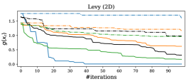
We have considered for the same four benchmark functions used in (González et al.,, 2017): ‘Forrester’ (1D), ‘Six-Hump Camel’ (2D), ‘Gold-Stein’ (2D) and ‘Levy’ (2D), and additionally ‘Rosenbrock5’ (5D) and ‘Hartman6’ (6D). These are minimization problems.999We converted them into maximizations so that the acquisition functions in Section 5 are well-defined. Each experiment starts with initial (randomly selected) duels and a total budget of duels are run. Further, each experiment is repeated 20 times with different initialization (the same for all methods) as in (González et al.,, 2017). We compare PBO based on GPL versus SkewGP using the three different acquisition functions described in Section 5: UCB, EIIG ( and ) and Thompson (denoted as TH). As before, we show plots of #iterations versus . In these experiments we optimize the kernel hyperparameters by maximising the marginal likelihood for both GPL and SkewGP.

|

|

|
|

|

|
| Forrester | Six Hump Camel | Gold Stein | Levy | Rosenbrock5 | Hartman6 | |
|---|---|---|---|---|---|---|
| GPL PBO | 557 | 2986 | 3346 | 4704 | 4314 | 5801 |
| SkewGP PBO | 102 | 2276 | 1430 | 1211 | 2615 | 2178 |
Figure 6 reports the performance of the different methods. Consistently across all benchmarks PBO-SkewGP outperforms PBO-GPL no matter the acquisition function. PBO-SkewGP has also a lower computational burden as showed in the Table at the bottom of Figure 6 that compares the median (over 80 trials, that is 20 trials times 4 acquisition functions) computational time per 100 iterations in seconds (on a standard laptop).
6.2 Mixed preferential-categorical BO
We examine now situations where certain unknown values of the inputs produce no-output preference and address it as a mixed preferential-categorical BO as described in Section 3.2. We consider again and assume that any input produces a non-valid output. Figure 7(left) shows , the location of the queried points101010The preferences are , , , , . and the no-valid zone (in grey). Figure 7(right) shows the predicted posterior preference function (and relative 95% credible region) computed according to SkewGP. We can see how SkewGP learns the non-valid region: the posterior mean is negative for and positive otherwise (the oscillations of the mean for capture the preferences). This is consistent with the likelihood in (10).

|
We consider now the following benchmark optimization problem proposed in (Sasena et al.,, 2002):
with and we assume that the input is valid if . We also assume that both the objective function and are unknown. The goal is to find the minimum: with optimal cost . Figure 8(left) shows the level curves of the objective function, the non-valid zone (grey bands) and the location of the minimizer (red star). We compare two approaches. The first approach uses PBO-SkewGP that minimizes the objective plus a penalty term, , that is non-zero in the non-valid region. Adding a penalty for non-valid inputs is the most common approach to deal with this type of problems. The second approach uses a SkewGP based mixed preferential-categorical BO (SkewGP-mixed) that accounts for the valid/non-valid points as in Section 3.2. Figure 8(right) shows the performance of the two compared methods, which is consistent across the three different acquisition functions: SkewGP-mixed converges more quickly to the optimum. This confirms that modelling directly this type of problems via the mixed preferential-categorical likelihood in (10) enables the model to fully exploit the available information. Also in this case, SkewGP allows us to compute the corresponding posterior exactly.


7 Conclusions
In this work we have shown that is possible to perform exact preferential Bayesian optimization by using Skew Gaussian processes. We have demonstrated that in the setting of preferential BO: (i) the Laplace’s approximation is very poor; (ii) given the strong skewness of the posterior, any approximation of the posterior that relies on a symmetric distribution will result to sub-optimal predictive performances and, therefore, slower convergence in PBO. We have also shown that we can extend this model to deal with mixed preferential-categorical Bayesian optimisation, while still providing the exact posterior. We envisage an immediate extension of our current approach. Many optimisation applications are subject to safety constraints, so that inputs cannot be freely chosen from the entire input space. This leads to so-called safe Bayesian optimization (Gotovos et al.,, 2015), that has been extended to safe preferential BO in (Sui et al.,, 2018). We plan to solve this problem exactly using SkewGP.
Appendix A Background on the Skew-Normal distribution
In this section we provide more details on the skew-normal distribution. See, e.g. Azzalini, (2013) for a complete reference on skew-normal distributions and their parametrizations.
A.1 Additive representations
The role of the latent dimension can be briefly explained as follows. Consider a random vector with as in (2) and define as the vector with distribution . The density of can be written as
where the first equality comes from a basic property of conditional distributions, see, e.g.(Azzalini,, 2013, Ch. 1.3), and the second equality is a consequence of the multivariate normal conditioning properties. Then we have that .
The previous representation provides an interesting point of view on the skew-Gaussian random vector, however the following representation turns out to be more practical for sampling from this distribution. Consider the independent random vectors and , the truncation below of . Then the random variable
is distributed as (1).
Proof.
We can show that the representation is equivalent to . Define and , where . Note that and . Then we have that and are independent. This can be verified by the fact that and are normally distributed with covariance which can be verified with algebraic computations. Finally note that is distributed as . ∎
The additive representation introduced above is used in Section 2.4 to draw samples from the distribution.
A.2 Closure properties
The Skew-Normal family has several interesting properties, see Azzalini, (2013, Ch.7) for details. Most notably, it is close under marginalization and affine transformations. Specifically, if we partition , where and with , then
| (11) |
Moreover, (Azzalini,, 2013, Ch.7) the conditional distribution is a unified skew-Normal, i.e.,
where
and .
In section 2.4 we exploit this property to obtain samples from the predictive posterior distribution at a new input given samples of the posterior at the training inputs.
A.3 Sampling from the posterior predictive distribution
Consider a test point and assume we have a sample from the posterior distribution . Consider the vector , which is distributed as , where
Then by using the marginalization property introduced above we obtain the formula in (5).
Appendix B Proofs of the results in the paper
Theorem 1
This proof is based on the proofs in (Durante,, 2019, Th.1 and Co.4). We aim to derive the posterior of . The joint distribution of is
| (12) |
where we have omitted the dependence on for easier notation. We note that
Therefore, we can write
| (13) |
with
and
Theorem 2
Consider the test point and the vector we have
and the predictive distribution is by definition
We can then apply Lemma 1 with and the likelihood which results in a posterior distribution
with
By exploiting the marginalization properties of the SUN distribution, see Section A.2, we obtain
| (14) |
Corollary 1
Proposition 1
As described in Section A.1, if we consider a random vector with and define as the vector with distribution , then it can be shown (Azzalini,, 2013, Ch. 7) that . This allows one to derive the following sampling scheme:
| (15) | ||||
where is the pdf of a multivariate Gaussian distribution truncated component-wise below . Then from the marginal (14) and the above sampling scheme (see Section A.3), we obtain the formulae in (15), main text.
Corollary 2
Appendix C Implementation
C.1 Laplace’s approximation
The Laplace’s approximation for preference learning was implemented as described in Chu and Ghahramani, (2005). We use standard Bayesian optimisation to optimise the hyper-parameters of the kernel by maximising the Laplace’s approximation of the marginal likelihood.
C.2 Skew Gaussian Process
C.3 Acquisition function optimisation
In sequential BO, our objective is to seek a new data point which will allow us to get closer to the maximum of the target function . Since can only be queried via preferences, this is obtained by optimizing w.r.t. a dueling acquisition function , where is the best point found so far, that is the point that has the highest probability of winning most of the duels (given the observed data ) and, therefore, it is the most likely point maximizing .
For both the models (Laplace’s approximation (GPL) and SkewGP) we compute the acquisition functions via Monte Carlo sampling from the posterior. In fact, although for GPL some analytical formulas are available (for instance for UCB), by using random sampling (2000 samples with fixed seed) for both GPL and SkewGP removes any advantage of SkewGP over GPL due to the additional exploration effect of Monte Carlo sampling. Computing in this way is very fast for both the models (for SkewGP this is due to lin-ess). We then optimize : (i) by computing for 5000 random generated value of (every time we use the same random points for both SkewGP and GPL); (ii) the best random instance is then used as initial guess for L-BFGS-B.
References
- Arellano and Azzalini, (2006) Arellano, R. B. and Azzalini, A. (2006). On the unification of families of skew-normal distributions. Scandinavian Journal of Statistics, 33(3):561–574.
- Azzalini, (2013) Azzalini, A. (2013). The skew-normal and related families, volume 3. Cambridge University Press.
- Bemporad and Piga, (2019) Bemporad, A. and Piga, D. (2019). Active preference learning based on radial basis functions. arXiv preprint arXiv:1909.13049.
- Benavoli et al., (2020) Benavoli, A., Azzimonti, D., and Piga, D. (2020). Skew Gaussian Processes for Classification. accepted to Machine Learning, arXiv preprint arXiv:2005.12987.
- Brochu et al., (2010) Brochu, E., Cora, V., and Freitas, N. D. (2010). A tutorial on Bayesian optimization of expensive cost functions, with application to active user modeling and hierarchical reinforcement learning. arXiv preprint arXiv:1012.2599.
- Brochu et al., (2008) Brochu, E., de Freitas, N., and Ghosh, A. (2008). Active preference learning with discrete choice data. In Advances in neural information processing systems, pages 409–416.
- Chernev et al., (2015) Chernev, A., Böckenholt, U., and Goodman, J. (2015). Choice overload: A conceptual review and meta-analysis. Journal of Consumer Psychology, 25(2):333–358.
- Chu and Ghahramani, (2005) Chu, W. and Ghahramani, Z. (2005). Preference learning with gaussian processes. In Proceedings of the 22nd International Conference on Machine Learning, ICML ’05, page 137–144, New York, NY, USA. Association for Computing Machinery.
- Durante, (2019) Durante, D. (2019). Conjugate Bayes for probit regression via unified skew-normal distributions. Biometrika, 106(4):765–779.
- Gessner et al., (2019) Gessner, A., Kanjilal, O., and Hennig, P. (2019). Integrals over gaussians under linear domain constraints. arXiv preprint arXiv:1910.09328.
- González et al., (2017) González, J., Dai, Z., Damianou, A., and Lawrence, N. D. (2017). Preferential bayesian optimization. In Proceedings of the 34th International Conference on Machine Learning-Volume 70, pages 1282–1291. JMLR. org.
- Gotovos et al., (2015) Gotovos, A., CH, E., Burdick, J. W., and EDU, C. (2015). Safe exploration for optimization with gaussian processes. In International Conference on Machine Learning (ICML).[Sui, Yue, and Burdick 2017] Sui, Y.
- Houlsby et al., (2011) Houlsby, N., Huszár, F., Ghahramani, Z., and Lengyel, M. (2011). Bayesian active learning for classification and preference learning. arXiv preprint arXiv:1112.5745.
- Mockus, (2012) Mockus, J. (2012). Bayesian approach to global optimization: theory and applications, volume 37. Springer Science & Business Media.
- Murray et al., (2010) Murray, I., Adams, R., and MacKay, D. (2010). Elliptical slice sampling. In Proceedings of the 13th International Conference on Artificial Intelligence and Statistics, pages 541–548, Chia, Italy. PMLR.
- O’Hagan and Leonard, (1976) O’Hagan, A. and Leonard, T. (1976). Bayes estimation subject to uncertainty about parameter constraints. Biometrika, 63(1):201–203.
- Rasmussen and Williams, (2006) Rasmussen, C. E. and Williams, C. K. (2006). Gaussian processes for machine learning. MIT press Cambridge, MA.
- Sadigh et al., (2017) Sadigh, D., Dragan, A. D., Sastry, S., and Seshia, S. A. (2017). Active preference-based learning of reward functions. In Robotics: Science and Systems.
- Sasena et al., (2002) Sasena, M. J., Papalambros, P., and Goovaerts, P. (2002). Exploration of metamodeling sampling criteria for constrained global optimization. Engineering optimization, 34(3):263–278.
- Siroker and Koomen, (2013) Siroker, D. and Koomen, P. (2013). A/B testing: The most powerful way to turn clicks into customers. John Wiley & Sons.
- Sui et al., (2018) Sui, Y., vincent Zhuang, Burdick, J., and Yue, Y. (2018). Stagewise safe Bayesian optimization with Gaussian processes. In Dy, J. and Krause, A., editors, Proceedings of the 35th International Conference on Machine Learning, volume 80 of Proceedings of Machine Learning Research, pages 4781–4789, Stockholmsmässan, Stockholm Sweden. PMLR.
- Thurstone, (1927) Thurstone, L. (1927). A law of comparative judgment. Psychological review, 34(4):273.
- Trinh and Genz, (2015) Trinh, G. and Genz, A. (2015). Bivariate conditioning approximations for multivariate normal probabilities. Statistics and Computing, 25(5):989–996.
- Zoghi et al., (2014) Zoghi, M., Whiteson, S., Munos, R., and Rijke, M. (2014). Relative upper confidence bound for the k-armed dueling bandit problem. In Proceedings of the 31st International Conference on Machine Learning, pages 10–18, Bejing, China.