Predicting the Reliability of an Image Classifier under Image Distortion
Abstract
In image classification tasks, deep learning models are vulnerable to image distortions i.e. their accuracy significantly drops if the input images are distorted. An image-classifier is considered “reliable” if its accuracy on distorted images is above a user-specified threshold. For a quality control purpose, it is important to predict if the image-classifier is unreliable/reliable under a distortion level. In other words, we want to predict whether a distortion level makes the image-classifier “non-reliable” or “reliable”. Our solution is to construct a training set consisting of distortion levels along with their “non-reliable” or “reliable” labels, and train a machine learning predictive model (called distortion-classifier) to classify unseen distortion levels. However, learning an effective distortion-classifier is a challenging problem as the training set is highly imbalanced. To address this problem, we propose two Gaussian process based methods to rebalance the training set. We conduct extensive experiments to show that our method significantly outperforms several baselines on six popular image datasets.
keywords:
Image classification; Reliability prediction; Image distortion; Imbalance classification; Gaussian process.1 Introduction
Many image classification models have assisted humans from daily ordinary tasks like shopping (Google Lens) and entertainment (FaceApp) to important jobs like healthcare (Calorie Mama) and authentication (BioID).
A well-known weakness of image-classifiers is that they are often vulnerable to image distortions i.e. their performance significantly drops if the input images are distorted [1]. As illustrated in Figure 1, a ResNet model achieved 99% accuracy on a set of CIFAR-10 images. When the images were slightly rotated, its accuracy dropped to 82%. It predicted wrong labels for rotated images although these images were easily recognized by humans. In practice, input images can be distorted in various forms e.g. rotated images due to an unstable camera, dark images due to a poor lighting condition, noisy images due to a rainy weather, etc.


For a quality control purpose, we need to evaluate the image-classifier under different distortion levels to check in which cases it is unreliable/reliable. As this task is very time- and cost-consuming, it is important to perform it automatically using a machine learning (ML) approach. In particular, we ask the question “can we predict the model reliability under an image distortion?”, and form it as a binary classification problem. Assume that we have an image-classifier and a set of labeled images (we call it verification set). We define the search space of distortion levels as follows: (1) each dimension of is a distortion type (e.g. rotation, brightness) and (2) each point is a distortion level (e.g. {rotation=20∘, brightness=0.5}), which is used to modify the images in to create a set of distorted images . The model is called “reliable” under a distortion level if ’s accuracy on is above a stipulated threshold , otherwise “non-reliable”. Recall the earlier example, if we choose the threshold , then the ResNet model is non-reliable under -rotation as its accuracy is only 82%. In other words, the distortion level -rotation has a label “non-reliable”. Our goal is to build a distortion-classifier that receives a distortion level and classifies it as (“non-reliable”) or (“reliable”). For simplicity, we treat “non-reliable” as negative label whereas “reliable” as positive label.
The process to train the distortion-classifier consists of three steps. (1) Construct a training set: a typical way to create a training set for is to randomly sample distortion levels from the search space and computing their corresponding labels. Given a , we compute the accuracy of the model on the set of distorted images . If , we assign a label “1”, otherwise a label “0”. As a result, we obtain a training set , where is an indicator function and is the sampling budget. We illustrate this procedure to construct the training set in Figure 2. (2) Rebalance the training set: using random distortion levels often leads to an imbalanced training set as a majority of them fall under negative class, especially when the threshold is high or model performance under distortion is generally poor. Thus, we need to rebalance using an imbalance handling technique like SMOTE [2], NearMiss [3], or generative models [4]. (3) Train the distortion-classifier: we use the rebalanced version of to train a ML predictive model e.g. neural network to classify unseen distortion levels.
Although current imbalance handling methods can rebalance the training data, they often suffer from generating false positive samples, leading to a sub-optimal training set for the distortion-classifier . In this paper, we improve the training set of with two contributions: (1) a Gaussian process (GP) based sampling technique to create a training set with a higher fraction of real positive samples and (2) a GP-based imbalance handling technique to further rebalance by generating more synthetic positive samples.

GP-based sampling: we consider the mapping from a distortion level to the model’s accuracy on the set of distorted images as a black-box, expensive function . The function is black-box as we do not know its expression, and is expensive as we have to measure the model’s accuracy over all distorted images in . We approximate using a GP [5] that is a popular method to model black-box, expensive functions. We use ’s predictive distribution to design an acquisition function to search for distortion levels that have a high chance to be a positive sample. We update the GP with new samples, and repeat the sampling process until the sampling budget is depleted. Finally, we obtain a training set .
GP-based imbalance handling: we use SMOTE on to generate synthetic positive samples. But, SMOTE often generates many false positive samples [6]. To solve this problem, we assign an uncertainty score for each synthetic positive sample via the variance function of a GP. We filter out synthetic samples whose uncertainty scores are high. This helps to reduce the false positive rate of SMOTE.
To summarize, we make the following contributions.
-
1.
We are the first to define the problem of Prediction of Model Reliability under Image Distortion, and propose a distortion-classifier to predict if the model is reliable under a distortion level.
-
2.
We propose a GP-based sampling technique to construct a training data for the distortion-classifier with an increased fraction of real positive samples.
-
3.
We propose a GP-based imbalance handling method to reduce the false positive rate when generating synthetic positive samples.
-
4.
We extensively evaluate our method on six benchmark image datasets, and compare it with several strong baselines. We show that it is significantly better than other methods.
-
5.
The significance of our work lies in providing ability to predict reliability of any image-classifier under a variety of distortions on any image dataset.
The remainder of the paper is organized as follows. In Section 2, related works on image distortion, model reliability, and imbalance classification are reviewed. Our main contributions are presented in Section 3, where we describe two GP-based methods for addressing class imbalance. Experimental results are discussed in Sections 4 while conclusions and future works are represented in Section 5.
2 Related Work
Image distortion. Most deep learning models are sensitive to image distortion, where a small amount of distortion can severely reduce their performance. Many methods have been proposed to detect and correct the distortion in the input images [7, 1], which can be categorized into two groups: non-reference and full-reference. The non-reference methods corrected the distortion without any direct comparison between the original and distorted images [8, 9]. Other works developed models that were robust to image distortion, where most of them fine-tuned the pre-trained models on a pre-defined set of distorted images [10, 11, 12]. While these methods focused on improving the model quality, which is useful for the model development phase, our work focuses on predicting the model reliability, which is useful for the quality control phase.
Model reliability prediction. Assessing the reliability of a ML model is an important step in the quality control process [13]. Existing works on model reliability focus on defect/bug prediction [14], where they classify a model as “defective” if its source code has bugs. A typical solution has three main steps [15, 16]. First, we collect both “clean” and “defective” code samples from the model repository to construct a training set. Second, we rebalance the training set. Finally, we train a ML predictive model with the rebalanced training set.
Some works target to other reliability aspects of a model such as relevance and reproducibility [17]. However, there is no work addressing the problem of model reliability prediction under image distortion.
Imbalance classification. As the problem of classification with imbalanced data has been studied for many years, the imbalance classification has a rich literature. Most existing methods are based on SMOTE (Synthetic Minority Oversampling Technology) [2], where the synthetic minority samples are generated by linearly combining two real minority samples. Several variants have been developed to address SMOTE weaknesses such as outlier and noisy [18, 19, 20, 21, 22]. Other approaches for rebalancing data are under-sampling techniques [3], ensemble methods [23, 24], and generative models [25, 26, 27].
3 Framework
3.1 Problem statement
Let be an image-classifier, be a set of labeled images (i.e. verification set), and be a set of image distortions e.g. rotation, brightness, etc. Each has a value range , where and are the lower and upper bounds. We define a compact subset of as a set of all possible values for image distortion (i.e. is the search space of all possible distortion levels).
We consider a mapping function , which receives a distortion level as input and returns the accuracy of on the set of distorted images as output. Here, each image is a distorted version of an original image , caused by the distortion level . Given a threshold , is considered “reliable” under if , otherwise “non-reliable”. Without any loss in generality, we treat “non-reliable” as negative label (i.e. class ) while “reliable” as positive label (i.e. class ).
Our goal is to build a distortion-classifier to classify any distortion level into positive or negative class.
3.2 Proposed method
The distortion-classifier is trained with three main steps. First, we create a training set , where is randomly sampled from and is the sampling budget. However, is often highly unbalanced, where the number of negative samples is much more than the number of positive samples. Second, we rebalance using an imbalance handling technique such as SMOTE or a generative model. Finally, we use the rebalanced version of to train that can be any ML predictive model e.g. random forest, neural network, etc.
We improve the quality of the training set by proposing two new approaches. First, instead of using random sampling method, we propose a GP-based sampling method to sample to construct . Second, we further rebalance using a novel GP-based imbalance handling technique.
3.2.1 GP-based sampling
Our goal is to sample more positive samples when constructing . To achieve this, we consider the mapping function as a black-box function and approximate it using a GP. We then use the GP predictive distribution to guide our sampling process. The detailed steps are described as follows.
-
1.
We initialize the training set with a small set of randomly sampled distortion levels and compute their function values , where is a small number i.e. (recall that is the sampling budget).
-
2.
We use to learn a GP to approximate . We assume that is a smooth function drawn from a GP, i.e. , where and are the mean and covariance functions. We compute the predictive distribution for at any point as a Gaussian distribution, with its mean and variance functions:
(1) (2) where is a vector with its -th element defined as and is a matrix of size with its -th element defined as .
-
3.
We iteratively update the training set by adding the new point until the sampling budget is depleted, and at each iteration we also update the GP. Instead of randomly sampling , we select by maximizing the following acquisition function :
(3) (4) where and are the predictive mean and standard deviation from Equations (1) and (2). The coefficient is computed following [28], where is the number of dimensions of the search space and is a small constant.
-
4.
We construct the training set , where is sampled using our acquisition function in Equation (4).
Our sampling strategy achieves two goals: (1) sampling where the model’s accuracy is higher than the threshold (i.e. large ) and (2) sampling where the model’s accuracy is highly uncertain (i.e. large ). As a result, we can efficiently find more positive samples. In the experiments, we show that our GP-based sampling method retrieves a much higher fraction of positive samples than the random sampling method.
Discussion. We want to highlight that our sampling strategy is very flexible. If is the minority class as in our setting, then we use . If is the minority class, then we can simply change it to .
3.2.2 GP-based imbalance handling
We further rebalance the training set by generating synthetic positive samples. Existing over-sampling methods such as SMOTE [2] and its variants [29] suffer from a high false positive rate. To address this problem, we propose a novel method combining SMOTE and GP. We call it SMOTE-GP.
We use SMOTE on to generate synthetic positive samples. Given a real positive sample , a new synthetic positive sample will be , where is another real positive sample and is a random number. We indicate the set of synthetic positive samples as . However, SMOTE tends to generate false positive samples as the line connecting two real positive samples crosses the negative region, as shown in Figure 3(a). Our goal is to reject such false positive samples.

When SMOTE generates a new synthetic positive sample , it simply assigns to label . But, SMOTE does not provide any confidence estimation for its assignment. However, if we had such a confidence measure, we could reject the synthetic sample whose confidence is low (i.e. its uncertainty is high).
To measure the uncertainty of a SMOTE assignment, we use the variance function of a GP. First, we retrieve the set of real positive samples in , we indicate this set as . Second, we train the GP using real positive samples in along with their function values. As the GP is trained with only real positive samples, it can approximate the generation process of SMOTE. Then, we compute an uncertainty score for each synthetic positive sample (recall is the set of synthetic positive samples generated by SMOTE):
| (5) |
where is the variance function of the GP, is a vector with its -th element being and is a matrix of size with its -th element being .
Finally, as measures the uncertainty of the synthetic positive sample , if is smaller than a threshold , we keep . Otherwise, we discard . The procedure of our SMOTE-GP is shown in Algorithm 1.
4 Experiments
4.1 Experiment settings
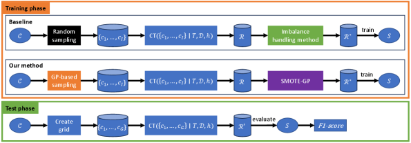
We recall steps involved in the training and test phases of our prediction task for model reliability under image distortion in Figure 4. We then provide their implementation details.
Search space of distortion levels . We predict the reliability of image-classifiers against six image distortions including geometry distortions [30], lighting distortion [31], and rain distortion [32]. We illustrate six distortion types in Figure 5. The value range of each image distortion is shown in Table 1. Note that our method is applicable to any distortion types as long as they can be defined by a range of values.

| Distortion | Domain | Description |
|---|---|---|
| Scale | Zoom in/out 0-30% | |
| Rotation | Rotate - | |
| Translation-X | Shift left/right 0-20% | |
| Translation-Y | Shift up/down 0-20% | |
| Darkness | Darken/brighten 0-30% | |
| Rain | : no rain, : a lot of rain |
Sampling method. While the baseline uses a random sampling, our method uses the GP-based sampling. After the sampling process, we obtain a set of distortion levels , where is the sampling budget.
Construction of training set . Given distortion levels , the module assigns label or for each (see Figure 2). It requires image-classifier , verification set , and reliability threshold .
For image-classifiers , we use five pre-trained models from [33] for image datasets MNIST, Fashion, CIFAR-10, CIFAR-100, and Tiny-ImageNet. They achieved similar accuracy as those reported in [34, 35, 36]. We also use the pre-trained ResNet50 model from the Keras library†††https://keras.io/api/applications/resnet/#resnet50-function for ImageNette‡‡‡https://www.tensorflow.org/datasets/catalog/imagenette. As pointed out by [12, 1], we expect that these image-classifiers will reduce their performance when evaluated on distorted images.
For each image dataset, we use 10% of its data samples to be the verification set . The size of , the accuracy of on , and the reliability threshold are shown in Table 2.
| Accuracy of | |||
|---|---|---|---|
| MNIST | 6,000 | 0.9967 | 0.90 |
| Fashion | 6,000 | 0.9908 | 0.75 |
| CIFAR-10 | 5,000 | 0.9902 | 0.85 |
| CIFAR-100 | 5,000 | 0.9340 | 0.65 |
| Tiny-ImageNet | 10,000 | 0.6275 | 0.45 |
| ImageNette | 1,000 | 0.8290 | 0.70 |
Imbalance handling method. As the training set is highly imbalanced, we rebalance it before training the distortion-classifier . We use SMOTE-GP and compare it with SOTA imbalance handling methods, including Cost-sensitive learning [37], under-sampling method NearMiss [3], over-sampling methods SMOTE [2] and AdaSyn [38], ensemble methods SPE [23] and MESA [24], and generative models GAN [27], VAE [25], CTGAN, and TVAE [26].
As our method is based on SMOTE, we also compare it with SMOTE variants, including SMOTE-Borderline [20], SMOTE-SVM [21], SMOTE-ENN [19], SMOTE-TOMEK [18], and SMOTE-WB [22]. To be fair, we use the source codes released by the authors or implemented in well-known public libraries. The details are provided in B.
Distortion-classifier . We train five popular ML predictive models with the rebalanced training set , including decision tree, random forest, logistic regression, support vector machine, and neural network. Each of them is a distortion-classifier. In the test phase, we report the averaged result of five distortion-classifiers.
Construction of test set . To evaluate the performance of distortion-classifiers, we need to construct a test set. We create a grid of distortion levels in . For each dimension, we use five points, resulting in 4,096 grid points in total. For each test point , we determine its label using the procedure in Figure 2. At the end, there are 4,096 test distortion levels along with their labels. We report the numbers of positive and negative test points in A.
Evaluation metric. We evaluate each distortion-classifier on the test set and compute the F1-score. As each imbalance handling method is combined with five ML predictive models to form five distortion-classifiers, we report the averaged F1-score. A higher F1-score means a better prediction.
We repeat each method three times with random seeds, and report the averaged F1-score. As the standard deviations are small (< 0.06), we do not report them to save space.
4.2 Comparison of sampling methods
We compare our GP-based sampling with the random sampling. From Figure 6, our GP-based sampling obtains many more positive points than the random sampling. For example, on CIFAR-10, among 600 sampled points, the random sampling obtains only 27 positive samples to construct the training set . In contrast, our GP-based sampling retrieves 130 positive samples to construct a more balanced .

4.3 Comparison of imbalance handling methods
We compare our imbalance handling method SMOTE-GP with current state-of-the-art imbalance handling methods. Our method has two versions: (1) SMOTE-GP combined with the random sampling and (2) SMOTE-GP combined with our GP-based sampling. We use the uncertainty threshold for CIFAR-10 and for other datasets.
Table 3 shows that our SMOTE-GP combined with our GP-based sampling is the best method and significantly outperforms other methods. Its improvements are around 5% on MNIST, 9% on Fashion, 3% on CIFAR-10, 8% on CIFAR-100, 6% on Tiny-ImageNet, and 14% on ImageNette.
| Sampling | Imbalance | M | F | C10 | C100 | T-IN | IN | |
|---|---|---|---|---|---|---|---|---|
| Standard | Random | None | 0.3657 | 0.2105 | 0.6507 | 0.4130 | 0.3587 | 0.6561 |
| Cost-sensitive | Random | Re-weight | 0.5478 | 0.3940 | 0.6938 | 0.5593 | 0.5256 | 0.6677 |
| Under-sampling | Random | RandomUnder | 0.2553 | 0.1467 | 0.5531 | 0.2824 | 0.2870 | 0.3989 |
| Random | NearMiss | 0.3358 | 0.1514 | 0.6588 | 0.4610 | 0.3443 | 0.6764 | |
| Over-sampling | Random | RandomOver | 0.6194 | 0.4554 | 0.7230 | 0.5939 | 0.5797 | 0.7063 |
| Random | SMOTE | 0.6157 | 0.4379 | 0.7310 | 0.5933 | 0.5658 | 0.7100 | |
| Random | Adasyn | 0.6090 | 0.4370 | 0.7306 | 0.5955 | 0.5663 | 0.7065 | |
| Ensemble | Random | SPE | 0.5237 | 0.2984 | 0.7269 | 0.5113 | 0.4816 | 0.6808 |
| Random | MESA | 0.4337 | 0.2120 | 0.6402 | 0.4394 | 0.3739 | 0.5802 | |
| Deep learning | Random | GAN | 0.3202 | 0.2186 | 0.5157 | 0.3358 | 0.3551 | 0.4739 |
| Random | VAE | 0.3831 | 0.2264 | 0.6635 | 0.4123 | 0.3821 | 0.6638 | |
| Random | CTGAN | 0.2958 | 0.1966 | 0.4124 | 0.2968 | 0.3144 | 0.3904 | |
| Random | TVAE | 0.3364 | 0.2124 | 0.5319 | 0.3365 | 0.3249 | 0.4673 | |
| Ours | Random | SMOTE-GP | 0.6356 | 0.4611 | 0.7433 | 0.6440 | 0.5856 | 0.7929 |
| GP-based | SMOTE | 0.6361 | 0.5327 | 0.7562 | 0.6525 | 0.5952 | 0.7988 | |
| GP-based | SMOTE-GP | 0.6635 | 0.5467 | 0.7616 | 0.6780 | 0.6381 | 0.8559 |
When using the random sampling, our SMOTE-GP is still better than other methods by 1-8%. Among imbalance handling baselines, SMOTE often achieves the best results. When SMOTE is combined with our GP-based sampling, its performance is improved significantly. This shows that our GP-based sampling is better than the random sampling.
In general, imbalance handling methods often improve the performance of the distortion-classifier, compared to the standard distortion-classifier. Over-sampling methods are always better than under-sampling methods. Deep learning methods based on generative models do not show any real benefit.
Comparison with SMOTE variants. We also compare our SMOTE-GP with imbalance handling methods based on SMOTE in Table 4. Our method is the best method while other SMOTE-based methods perform similarly.
| MNIST | Fashion | CIFAR-10 | CIFAR-100 | Tiny-ImageNet | ImageNette | |
|---|---|---|---|---|---|---|
| SMOTE | 0.6157 | 0.4379 | 0.7310 | 0.5933 | 0.5658 | 0.7100 |
| SMOTE-Borderline | 0.6118 | 0.4313 | 0.7246 | 0.5924 | 0.5673 | 0.7057 |
| SMOTE-SVM | 0.6120 | 0.4231 | 0.7335 | 0.6020 | 0.5711 | 0.7187 |
| SMOTE-ENN | 0.6046 | 0.3931 | 0.6752 | 0.5504 | 0.5213 | 0.6744 |
| SMOTE-TOMEK | 0.6155 | 0.4381 | 0.7312 | 0.5931 | 0.5658 | 0.7096 |
| SMOTE-WB | 0.6210 | 0.4511 | 0.7276 | 0.5859 | 0.5659 | 0.7079 |
| SMOTE-GP (Ours) | 0.6635 | 0.5467 | 0.7616 | 0.6780 | 0.6381 | 0.8559 |
4.4 Ablation study
We conduct further experiments on CIFAR-10 to analyze our method under different settings.
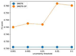
Uncertainty threshold . Our SMOTE-GP uses the uncertainty threshold to filter out false positive synthetic samples. We investigate how different values for affect our performance.
Figure 7 shows that our SMOTE-GP is always better than SMOTE with a large range of values. When is too small (i.e. ), it may drop its F1-score as most of synthetic positive samples are filtered out. When is too large (i.e. ), it may also reduce its F1-score since many false positive samples are introduced.
Sampling budget . We investigate the effect of the number of sampling queries (i.e. the size of the sampling budget ) on the performance of our method.
Figure 8 shows that both methods improve as the number of sampling queries increase as expected. More queries result in more training data and more chance to get positive samples. However, our SMOTE-GP is always better than SMOTE by a large margin.

Reliability threshold . We investigate how our performance is changed with different reliability thresholds .
Figure 9 shows that both methods reduce their F1-scores when the reliability threshold becomes larger as the image-classifier is reliable under fewer distortion levels (i.e. fewer positive samples). This leads to a very highly imbalanced training set .

Visualization. For a quantitative evaluation, we use t-SNE [39] to visualize the synthetic positive samples generated by each method. From Figure 10, SMOTE and its variants generate noisy synthetic samples in two situations. Only our SMOTE-GP avoids these problems.

5 Conclusion
Predicting model reliability is an important task in the quality control process. In this paper, we solve this task in the context of image distortion i.e. we predict if an image-classifier is unreliable/reliable under a distortion level. We form this task as a binary classification process with three main steps: (1) construct a training set, (2) rebalance the training set, and (3) train a distortion-classifier. As the training set is highly imbalanced, we propose two methods to handle the imbalance: (1) a GP-based sampling and (2) SMOTE-GP.
In the GP-based sampling, we approximate the black-box function mapping from a distortion level to the model’s accuracy on distorted images using GP. We then leverage the GP’s mean and variance to form our sampling process.
In the SMOTE-GP method, we compute an uncertainty score for each synthetic positive sample. We then filter out ones whose uncertainty scores are higher than a threshold.
We demonstrate the benefits of our method on six image datasets, where it greatly outperforms other baselines.
References
- [1] X. Li, B. Zhang, P. Sander, J. Liao, Blind geometric distortion correction on images through deep learning, in: CVPR, 2019, pp. 4855–4864.
- [2] N. Chawla, K. Bowyer, L. Hall, P. Kegelmeyer, SMOTE: synthetic minority over-sampling technique, Journal of Artificial Intelligence Research 16 (2002) 321–357.
- [3] I. Mani, J. Zhang, kNN approach to unbalanced data distributions: a case study involving information extraction, in: ICML Workshop, Vol. 126, 2003, pp. 1–7.
- [4] V. Sampath, I. Maurtua, J. J. Aguilar Martin, A. Gutierrez, A survey on generative adversarial networks for imbalance problems in computer vision tasks, Journal of Big Data 8 (2021) 1–59.
- [5] B. Shahriari, K. Swersky, Z. Wang, R. Adams, N. Freitas, Taking the human out of the loop: A review of bayesian optimization, Proceedings of the IEEE 104 (1) (2016) 148–175.
- [6] A. Fernández, S. Garcia, F. Herrera, N. Chawla, SMOTE for learning from imbalanced data: progress and challenges, marking the 15-year anniversary, Journal of Artificial Intelligence Research 61 (2018) 863–905.
- [7] N. Ahn, B. Kang, K.-A. Sohn, Image distortion detection using convolutional neural network, in: IEEE Asian Conference on Pattern Recognition (ACPR), 2017, pp. 220–225.
- [8] L. Kang, P. Ye, Y. Li, D. Doermann, Convolutional neural networks for no-reference image quality assessment, in: CVPR, 2014, pp. 1733–1740.
- [9] S. Bosse, D. Maniry, T. Wiegand, W. Samek, A deep neural network for image quality assessment, in: IEEE International Conference on Image Processing (ICIP), 2016, pp. 3773–3777.
- [10] Y. Zhou, S. Song, N.-M. Cheung, On classification of distorted images with deep convolutional neural networks, in: IEEE International Conference on Acoustics, Speech and Signal Processing (ICASSP), 2017, pp. 1213–1217.
- [11] S. Dodge, L. Karam, Quality robust mixtures of deep neural networks, IEEE Transactions on Image Processing 27 (11) (2018) 5553–5562.
- [12] M. T. Hossain, S. W. Teng, D. Zhang, S. Lim, G. Lu, Distortion robust image classification using deep convolutional neural network with discrete cosine transform, in: IEEE International Conference on Image Processing (ICIP), 2019, pp. 659–663.
- [13] F. Thung, S. Wang, D. Lo, L. Jiang, An empirical study of bugs in machine learning systems, in: International Symposium on Software Reliability Engineering, 2012, pp. 271–280.
- [14] F. Jafarinejad, K. Narasimhan, M. Mezini, NerdBug: automated bug detection in neural networks, in: International Workshop on AI and Software Testing/Analysis, 2021, pp. 13–16.
- [15] J. Wang, C. Zhang, Software reliability prediction using a deep learning model based on the RNN encoder–decoder, Reliability Engineering & System Safety 170 (2018) 73–82.
- [16] G. Giray, K. E. Bennin, Ö. Köksal, Ö. Babur, B. Tekinerdogan, On the use of deep learning in software defect prediction, Journal of Systems and Software 195 (2023) 111537.
- [17] M. M. Morovati, A. Nikanjam, F. Khomh, Z. M. Jiang, Bugs in machine learning-based systems: a faultload benchmark, Empirical Software Engineering 28 (3) (2023) 62.
- [18] G. Batista, A. Bazzan, M. C. Monard, et al., Balancing training data for automated annotation of keywords: a case study, WoB 3 (2003) 10–8.
- [19] G. Batista, R. Prati, M. C. Monard, A study of the behavior of several methods for balancing machine learning training data, ACM SIGKDD Explorations Newsletter 6 (1) (2004) 20–29.
- [20] H. Han, W.-Y. Wang, B.-H. Mao, Borderline-SMOTE: a new over-sampling method in imbalanced data sets learning, in: International Conference on Intelligent Computing, 2005, pp. 878–887.
- [21] H. Nguyen, E. Cooper, K. Kamei, Borderline over-sampling for imbalanced data classification, International Journal of Knowledge Engineering and Soft Data Paradigms 3 (1) (2011) 4–21.
- [22] F. Sağlam, M. A. Cengiz, A novel SMOTE-based resampling technique trough noise detection and the boosting procedure, Expert Systems with Applications 200 (2022) 117023.
- [23] Z. Liu, W. Cao, Z. Gao, J. Bian, H. Chen, Y. Chang, T.-Y. Liu, Self-paced ensemble for highly imbalanced massive data classification, in: ICDE, 2020, pp. 841–852.
- [24] Z. Liu, P. Wei, J. Jiang, W. Cao, J. Bian, Y. Chang, MESA: Boost Ensemble Imbalanced Learning with MEta-SAmpler, in: NeurIPS, Vol. 33, 2020, pp. 14463–14474.
- [25] D. Kingma, M. Welling, et al., An introduction to variational autoencoders, Foundations and Trends in Machine Learning 12 (4) (2019) 307–392.
- [26] L. Xu, M. Skoularidou, A. Cuesta-Infante, K. Veeramachaneni, Modeling tabular data using Conditional GAN, in: NeurIPS, Vol. 32, 2019, pp. 7335–7345.
- [27] I. Goodfellow, J. Pouget-Abadie, M. Mirza, B. Xu, D. Warde-Farley, S. Ozair, A. Courville, Y. Bengio, Generative adversarial networks, Communications of the ACM 63 (11) (2020) 139–144.
- [28] N. Srinivas, A. Krause, S. Kakade, M. Seeger, Information-theoretic regret bounds for gaussian process optimization in the bandit setting, IEEE Transactions on Information Theory 58 (5) (2012) 3250–3265.
- [29] G. Kovács, Smote-variants: A python implementation of 85 minority oversampling techniques, Neurocomputing 366 (2019) 352–354.
- [30] S. Gopakumar, S. Gupta, S. Rana, V. Nguyen, S. Venkatesh, Algorithmic assurance: An active approach to algorithmic testing using bayesian optimisation, in: NIPS, 2018, pp. 5466–5474.
- [31] H. Sellahewa, S. Jassim, Image-quality-based adaptive face recognition, IEEE Transactions on Instrumentation and measurement 59 (4) (2010) 805–813.
- [32] P. Patil, S. Gupta, S. Rana, S. Venkatesh, Video restoration framework and its meta-adaptations to data-poor conditions, in: ECCV, 2022, pp. 143–160.
- [33] D. Nguyen, S. Gupta, K. Do, S. Venkatesh, Black-box few-shot knowledge distillation, in: ECCV, 2022.
- [34] Y. Tian, D. Krishnan, P. Isola, Contrastive representation distillation, in: ICLR, 2020.
- [35] D. Wang, Y. Li, L. Wang, B. Gong, Neural Networks Are More Productive Teachers Than Human Raters: Active Mixup for Data-Efficient Knowledge Distillation from a Blackbox Model, in: CVPR, 2020, pp. 1498–1507.
- [36] P. Bhat, E. Arani, B. Zonooz, Distill on the go: Online knowledge distillation in self-supervised learning, in: CVPR Workshop, 2021, pp. 2678–2687.
- [37] N. Thai-Nghe, Z. Gantner, L. Schmidt-Thieme, Cost-sensitive learning methods for imbalanced data, in: IJCNN, 2010, pp. 1–8.
- [38] H. He, Y. Bai, E. Garcia, S. Li, ADASYN: Adaptive synthetic sampling approach for imbalanced learning, in: IJCNN, 2008, pp. 1322–1328.
- [39] L. Van der Maaten, G. Hinton, Visualizing data using t-SNE, Journal of Machine Learning Research 9 (11) (2008) 2579–2605.
Appendix A Test set
Table 5 reports the numbers of negative and positive samples in the test set , which is used to evaluate the performance of distortion-classifiers (see Figure 4).
| Dataset | #negative | #positive |
|---|---|---|
| MNIST | 3,957 | 139 |
| Fashion | 4,017 | 79 |
| CIFAR-10 | 3,884 | 212 |
| CIFAR-100 | 3,977 | 119 |
| Tiny-ImageNet | 3,991 | 105 |
| ImageNette | 3,940 | 156 |
Appendix B Implementation of baselines
To be fair, when comparing with other methods, we use their source code released by the authors or their implementation in well-known public libraries. Table 6 shows the link to the implementation of each baseline.
| Method | Implementation link |
|---|---|
| Re-weight | https://scikit-learn.org/stable/ |
| RandomUnder | https://imbalanced-learn.org/stable/ |
| NearMiss | |
| RandomOver | |
| SMOTE | |
| SMOTE-Borderline | |
| SMOTE-SVM | |
| SMOTE-ENN | |
| SMOTE-TOMEK | |
| Adasyn | |
| SMOTE-WB | https://github.com/analyticalmindsltd/smote_variants |
| SPE | https://github.com/ZhiningLiu1998/imbalanced-ensemble |
| MESA | https://github.com/ZhiningLiu1998/mesa |
| GAN | https://github.com/dialnd/imbalanced-algorithms |
| VAE | https://github.com/dialnd/imbalanced-algorithms |
| CTGAN | https://github.com/sdv-dev/CTGAN |
| TVAE | https://github.com/sdv-dev/CTGAN |