Predicting Online Item-choice Behavior:
A Shape-restricted Regression Approach

A number of prior studies have aimed at predicting users’ purchase behavior on e-commerce websites [10]. Mainstream research has applied stochastic or statistical models for predicting purchase sessions [5, 23, 30, 31, 36, 41, 46], but these approaches do not consider which items users choose.

Various machine learning methods have been used to predict online item-choice behavior, including logistic regression [12, 53], association rule mining [37], support vector machines [38, 53], ensemble learning methods [25, 26, 39, 52, 54], and artificial neural networks [21, 47, 50]. Tailored statistical models have also been proposed. For instance, Moe [29] devised a two-stage multinomial logit model that separates the decision-making process into item views and purchase decisions. Yao et al. [51] proposed a joint framework consisting of user-level factor estimation and item-level factor aggregation based on the buyer decision process. Borges and Levener [6] used Markov chain models to estimate the probability of the next link choice of a user.

These prior studies effectively utilized clickstream data in various prediction methods and showed that consideration of time-evolving user behavior is crucial for precise prediction of online item-choice behavior. We therefore focused on user PV sequences to estimate item-choice probabilities on e-commerce websites. Moreover, we evaluated the prediction performance of our method by comparison with machine learning methods that have commonly been used in prior studies.

In many practical situations, prior information is known about the relationship between explanatory and response variables. For instance, utility functions can be assumed to be increasing and concave according to economic theory [28], and option pricing functions to be monotone and convex according to finance theory [3]. Shape-restricted regression fits a nonparametric function to a set of given observations under shape restrictions such as monotonicity, convexity, concavity, or unimodality [8, 15, 16, 48].

Isotonic regression is the most common method for shape-restricted regression. In general, isotonic regression is the problem of estimating a real-valued monotone (non-decreasing or non-increasing) function with respect to a given partial order of observations [35]. Some regularization techniques [14, 44] and estimation algorithms [17, 35, 43] have been proposed for isotonic regression.

One of the greatest advantages of shape-restricted regression is that it mitigates overfitting, thereby improving prediction performance of regression models [4]. To utilize this advantage, Iwanaga et al. [19] devised a shape-restricted optimization model for estimating item-choice probabilities on e-commerce websites. Along similar lines, we propose a shape-restricted optimization model based on order relations of PV sequences to improve prediction performance.

Table I gives an example of a PV history for six user–item pairs. For instance, user $u_{1}$ viewed the page for item $i_{2}$ once on each of April 1 and 3. We focus on user choices (e.g., revisit and purchase) on April 4, which we call the base date. For instance, user $u_{1}$ chose item $i_{4}$ rather than item $i_{2}$ on the base date. We suppose for each user–item pair that recency and frequency are characterized by the last PV day and the total number of PVs, respectively. As shown in the table, the PV history can be summarized by the recency–frequency combination $(r,f)\in R\times F$, where $R$ and $F$ are index sets representing recency and frequency, respectively.

Let $n_{rf}$ be the number of user–item pairs having $(r,f)\in R\times F$, and set $q_{rf}$ to the number of choices occurring by user–item pairs that have $(r,f)\in R\times F$ on the base date. In the case of Table I, the empirical probability table is calculated as

where, for reasons of expediency, $\hat{x}_{rf}:=0$ for $(r,f)\in R\times F$ with $n_{rf}=0$.

It is reasonable to assume that the recency and frequency of user–item pairs are positively associated with user item-choice probabilities. To estimate user item-choice probabilities $x_{rf}$ for all recency–frequency combinations $(r,f)\in R\times F$, the two-dimensional monotonicity model [19] minimizes the weighted sum of squared errors under monotonicity constraints with respect to recency and frequency.

Note, however, that PV histories are often indistinguishable according to recency and frequency. A typical example is the set of user–item pairs $(u_{2},i_{3})$, $(u_{2},i_{4})$, and $(u_{3},i_{2})$ in Table I; although their PV histories are actually different, they have the same value $(r,f)=(3,3)$ for recency–frequency combinations. As described in the next section, we exploit the PV sequence to distinguish between such PV histories.

The PV sequence for each user–item pair represents a time series of the number of PVs, and is written as

where $v_{j}$ is the number of PVs $j$ periods earlier for $j=1,2,\ldots,n$ (see Table I). Note that sequence terms are arranged in reverse chronological order, so $v_{j}$ moves into the past as index $j$ increases.

Throughout the paper, we express sets of consecutive integers as

where $[m_{1},m_{2}]=\emptyset$ when $m_{1}>m_{2}$. The set of possible PV sequences is defined as

where $m$ is the maximum number of PVs in each period, and $n$ is the number of periods considered.

Our objective is to estimate item-choice probabilities $x_{\bm{v}}$ for all PV sequences $\bm{v}\in\Gamma$. However, the huge number of PV sequences makes it extremely difficult to accurately estimate such probabilities. In the case of $(n,m)=(|R|,|F|)=(5,6)$ for instance, the number of different PV sequences is $(m+1)^{n}=16{,}807$, whereas the number of recency–frequency combinations is only $|R|\cdot|F|=30$. To avoid this difficulty, we effectively utilize monotonicity constraints on item-choice probabilities as in the optimization model (9)–(12). In the next section, we introduce three operations underlying the development of the monotonicity constraints.

From the perspective of frequency, it is reasonable to assume that item-choice probability increases as the number of PVs in a particular period increases. To formulate this, we define the following operation:

For instance, we have $\texttt{Up}((0,1,1),1)=(1,1,1)$, and $\texttt{Up}((1,1,1),2)=(1,2,1)$. Since this operation increases PV frequencies, the monotonicity constraint $x_{(0,1,1)}\leq x_{(1,1,1)}\leq x_{(1,2,1)}$ should be satisfied by item-choice probabilities.

From the perspective of recency, we assume that more-recent PVs have a larger effect on increasing item-choice probability. To formulate this, we consider the following operation for moving one PV from an old period to a new period:

For instance, we have $\texttt{Move}((1,1,1),2,3)=(1,2,0)$, and $\texttt{Move}((1,2,0),1,2)=(2,1,0)$. Because this operation increases the number of recent PVs, item-choice probabilities should satisfy the monotonicity constraint $x_{(1,1,1)}\leq x_{(1,2,0)}\leq x_{(2,1,0)}$.

The PV sequence $\bm{v}=(1,1,1)$ represents a user’s continued interest in a certain item over three periods. In contrast, the PV sequence $\bm{v}=(1,2,0)$ implies that a user’s interest decreased over the two most-recent periods. In this sense, the monotonicity constraint $x_{(1,1,1)}\leq x_{(1,2,0)}$ may not be validated. Accordingly, we define the following alternative operation, which exchanges numbers of PVs to increase the number of recent PVs:

We thus have $\texttt{Swap}((1,0,2),2,3)=(1,2,0)$ because $v_{2}<v_{3}$, and $\texttt{Swap}((1,2,0),1,2)=(2,1,0)$ because $v_{1}<v_{2}$. Since this operation increases the number of recent PVs, item-choice probabilities should satisfy the monotonicity constraint $x_{(1,0,2)}\leq x_{(1,2,0)}\leq x_{(2,1,0)}$. Note that the monotonicity constraint $x_{(1,1,1)}\leq x_{(1,2,0)}$ is not implied by this operation.

Let $U\subseteq\Gamma$ be a subset of PV sequences. The image of each operation is then defined as

We define $\texttt{UM}(U):=\texttt{Up}(U)\cup\texttt{Move}(U)$ for $U\subseteq\Gamma$. The following definition states that the binary relation $\bm{u}\prec_{\texttt{UM}}\bm{v}$ holds when $\bm{u}$ can be transformed into $\bm{v}$ by repeated application of Up and Move:

Similarly, we define $\texttt{US}(U):=\texttt{Up}(U)\cup\texttt{Swap}(U)$ for $U\subseteq\Gamma$. Then, the binary relation $\bm{u}\prec_{\texttt{US}}\bm{v}$ holds when $\bm{u}$ can be transformed into $\bm{v}$ by repeated application of Up and Swap.

To prove properties of these binary relations, we can use the lexicographic order, which is a well-known linear order [40]:

Each application of Up, Move, and Swap makes a PV sequence greater in the lexicographic order. Therefore, we can obtain the following lemma:

The following theorem states that a partial order of PV sequences is derived by operations Up and Move.

We can similarly prove the following theorem for operations Up and Swap:

Let $n_{\bm{v}}$ be the number of user–item pairs that have the PV sequence $\bm{v}\in\Gamma$. Also, $q_{\bm{v}}$ is the number of choices arising from user–item pairs having $\bm{v}\in\Gamma$ on the base date. Similarly to Eq. (8), we can calculate empirical item-choice probabilities as

Our shape-restricted optimization model minimizes the weighted sum of squared errors subject to the monotonicity constraint:

where $\bm{u}\prec\bm{v}$ in Eq. (15) is defined by one of the partial orders $\prec_{\texttt{UM}}$ or $\prec_{\texttt{US}}$.

The monotonicity constraint (15) enhances the estimation accuracy of item-choice probabilities. In addition, our shape-restricted optimization model can be used in a post-processing step to improve prediction performance of other machine learning methods. Specifically, we first compute item-choice probabilities using a machine learning method and then substitute the computed values into $(\hat{x}_{\bm{v}})_{\bm{v}\in\Gamma}$ to solve the optimization model (14)–(16). Consequently, we can obtain item-choice probabilities corrected by the monotonicity constraint (15). Section VI-D illustrates the usefulness of this approach.

However, since $|\Gamma|=(m+1)^{n}$, it follows that the number of constraints in Eq. (15) is $\mathcal{O}((m+1)^{2n})$, which can be extremely large. When $(n,m)=(5,6)$, for instance, we have $(m+1)^{2n}=282{,}475{,}249$. The next section describes how we mitigate this difficulty by removing redundant constraints in Eq. (15).

A poset $(\Gamma,\preceq)$ can be represented by a directed graph $(\Gamma,E)$, where $\Gamma$ and $E\subseteq\Gamma\times\Gamma$ are sets of nodes and directed edges, respectively. Each directed edge $(\bm{u},\bm{v})\in E$ in this graph corresponds to the order relation $\bm{u}\prec\bm{v}$, so the number of directed edges coincides with the number of constraints in Eq. (15).

Figs. 1 and 2 show directed graph representations of posets $(\Gamma,\preceq_{\texttt{UM}})$ and $(\Gamma,\preceq_{\texttt{US}})$, respectively. Each edge in Figs. 1(a) and 2(a) corresponds to one of the operations Up, Move, or Swap. Edge $(\bm{u},\bm{v})$ is red if $\bm{v}\in\texttt{Up}(\{\bm{u}\})$ and black if $\bm{v}\in\texttt{Move}(\{\bm{u}\})$ or $\bm{v}\in\texttt{Swap}(\{\bm{u}\})$. The directed graphs in Figs. 1(a) and 2(a) can be easily created.

Suppose there are three edges

In this case, edge $(\bm{u},\bm{v})$ is implied by the other edges due to the transitivity of partial order

or, equivalently,

As a result, edge $(\bm{u},\bm{v})$ is redundant and can be removed from the directed graph.

A transitive reduction, also known as a Hasse diagram, of a directed graph $(\Gamma,E)$ is its subgraph $(\Gamma,E^{*})$ such that all redundant edges are removed using the transitivity of partial order [2]. Figs. 1(b) and 2(b) show transitive reductions of the directed graphs shown in Figs. 1(a) and 2(a), respectively. By computing transitive reductions, the number of edges is reduced from 90 to 42 in Fig. 1, and from 81 to 46 in Fig. 2. This transitive reduction is known to be unique [2].

The transitive reduction $(\Gamma,E^{*})$ is characterized by the following lemma [40]:

The basic strategy in general-purpose algorithms for transitive reduction involves the following steps:

• •

  Step 1: An exhaustive directed graph $(\Gamma,E)$ is generated from a given poset $(\Gamma,\preceq)$.

• •

  Step 2: The transitive reduction $(\Gamma,E^{*})$ is computed from the directed graph $(\Gamma,E)$ using Lemma 2.

Various algorithms for speeding up the computation in Step 2 have been proposed. Recall that $|\Gamma|=(m+1)^{n}$ in our situation. Warshall’s algorithm [49] has time complexity $\mathcal{O}((m+1)^{3n})$ for completing Step 2 [40]. By using a sophisticated algorithm for fast matrix multiplication, this time complexity can be reduced to $\mathcal{O}((m+1)^{2.3729n})$ [24].

However, such general-purpose algorithms are clearly inefficient, especially when $n$ is very large, and Step 1 requires a huge number of computations. To resolve this difficulty, we devised specialized algorithms for directly constructing a transitive reduction.

Let $(\Gamma,E^{*}_{\texttt{UM}})$ be a transitive reduction of a directed graph $(\Gamma,E_{\texttt{UM}})$ representing the poset $(\Gamma,\preceq_{\texttt{UM}})$. Then, the transitive reduction can be characterized by the following theorem:

Theorem 3 gives a constructive algorithm that directly computes the transitive reduction $(\Gamma,E^{*}_{\texttt{UM}})$ without generating an exhaustive directed graph $(\Gamma,E)$. Our algorithm is based on the breadth-first search [11]. Specifically, we start with a node list $L=\{(0,0,\ldots,0)\}\subseteq\Gamma$. At each iteration of the algorithm, we choose $\bm{u}\in L$, enumerate $\bm{v}\in\Gamma$ such that $(\bm{u},\bm{v})\in E^{*}_{\texttt{UM}}$, and add these nodes to $L$.

Table II shows this enumeration process for $\bm{u}=(0,2,1)$ with $(n,m)=(3,2)$. The operations Up and Move generate

which amounts to searching edges $(\bm{u},\bm{v})$ in Fig. 1(a). We next check whether each $\bm{v}$ satisfies conditions (UM1) or (UM2) in Theorem 3. As shown in Table II, we choose

and add them to list $L$; this amounts to enumerating edges $(\bm{u},\bm{v})$ in Fig. 1(b).

Appendix B-A presents pseudocode for our constructive algorithm (Algorithm 1). Recalling the time complexity analysis of the breadth-first search [11], one readily sees that the time complexity of Algorithm 1 is $\mathcal{O}(n(m+1)^{n})$, which is much smaller than $\mathcal{O}((m+1)^{2.3729n})$ as achieved by the general-purpose algorithm [24], especially when $n$ is very large.

Next, we focus on the transitive reduction $(\Gamma,E^{*}_{\texttt{US}})$ of a directed graph $(\Gamma,E_{\texttt{US}})$ representing the poset $(\Gamma,\preceq_{\texttt{US}})$. The transitive reduction can then be characterized by the following theorem:

Theorem 4 also gives a constructive algorithm for computing the transitive reduction $(\Gamma,E^{*}_{\texttt{US}})$. Let us again consider $\bm{u}=(0,2,1)$ as an example with $(n,m)=(3,2)$. As shown in Table III, operations Up and Swap generate

and we choose

(see also Figs. 2(a) and 2(b)).

Appendix B-B presents pseudocode for our constructive algorithm (Algorithm 2). Its time complexity is estimated to be $\mathcal{O}(n^{2}(m+1)^{n})$, which is larger than that of Algorithm 1 but much smaller than that of the general-purpose algorithm [24], especially when $n$ is very large.

We compared the performance of the methods listed in Table IV. All computations were performed on an Apple MacBook Pro computer with an Intel Core i7-5557U CPU (3.10 GHz) and 16 GB of memory.

The optimization models (9)–(12) and (14)–(16) were solved using OSQP³³3https://osqp.org/docs/index.html [42], a numerical optimization package for solving convex quadratic optimization problems. As in Table I, daily-PV sequences were calculated for each user–item pair, where $m$ is the maximum number of daily PVs and $n$ is the number of terms (past days) in the PV sequence. In this process, all PVs from more than $n$ days earlier were added to the number of PVs $n$ days earlier, and numbers of daily PVs exceeding $m$ were rounded down to $m$. Similarly, the recency–frequency combinations $(r,f)\in R\times F$ were calculated using daily PVs as in Table I, where $(|R|,|F|)=(n,m)$.

Other machine learning methods (LR, ANN, and RF) were respectively implemented using the LogisticRegressionCV, MLPRegressor, and RandomForestRegressor functions in scikit-learn, a Python library of machine learning tools. Related hyperparameters were tuned through 3-fold cross-validation according to the parameter settings in a benchmark study [34]. These machine learning methods employed the PV sequence $(v_{1},v_{2},\ldots,v_{n})$ as $n$ input variables for computing item-choice probabilities. We standardized each input variable and performed undersampling to improve prediction performance.

There are five pairs of training and validation sets of clickstream data in the preprocessed dataset [27]. As shown in Table V, each training period is 90 days, and the next day is the validation period. The first four pairs of training and validation sets, which we call the training set, were used for model estimation, and the fifth pair was used for performance evaluation. To examine how sample size affects prediction performance, we prepared small-sample training sets by randomly choosing user–item pairs from the original training set. Here, the sampling rates are 0.1%, 1%, and 10%, and the original training set is referred to as the full sample. Note that the results were averaged over 10 trials for the sampled training sets.

We considered the top-$N$ selection task to evaluate prediction performance. Specifically, we focused on items that were viewed by a particular user during a training period. From among these items, we selected $I_{\rm sel}$, a set of top-$N$ items for the user according to estimated item-choice probabilities. The most-recently viewed items were selected when two or more items had the same choice probability. Let $I_{\rm view}$ be the set of items viewed by the user in the validation period. Then, the F1 score is defined by the harmonic average of $\mbox{\emph{Recall}}:=|I_{\rm sel}\cap I_{\rm view}|/|I_{\rm view}|$ and $\mbox{\emph{Precision}}:=|I_{\rm sel}\cap I_{\rm view}|/|I_{\rm sel}|$ as

In the following sections, we examine F1 scores averaged over all users. The percentage of user–item pairs leading to item choices is only 0.16%.

We generated constraints in Eq. (15) based on the following three directed graphs:

• •

  Case 1 (Enumeration): All edges $(\bm{u},\bm{v})$ satisfying $\bm{u}\prec\bm{v}$ were enumerated.

• •

  Case 2 (Operation): Edges corresponding to operations Up, Move, and Swap were generated as in Figs. 1(a) and 2(a).

• •

  Case 3 (Reduction): Transitive reduction was computed using our algorithms as in Figs. 1(b) and 2(b).

Table VI shows the problem size of our PV sequence model (14)–(16) for some $(n,m)$ settings of the PV sequence. Here, the “#Vars” column shows the number of decision variables (i.e., $(m+1)^{n}$), and the subsequent columns show the number of constraints in Eq. (15) for the three cases mentioned above.

The number of constraints grew rapidly as $n$ and $m$ increased in the enumeration case. In contrast, the number of constraints was always kept smallest by the transitive reduction among the three cases. When $(n,m)=(5,6)$, for instance, transitive reductions reduced the number of constraints in the operation case to $63798/195510\approx 32.6\%$ for SeqUM and $85272/144060\approx 59.2\%$ for SeqUS.

The number of constraints was larger for SeqUM than for SeqUS in the enumeration and operation cases. In contrast, the number of constraints was often smaller for SeqUM than for SeqUS in the reduction case. Thus, the transitive reduction had a greater impact on SeqUM than on SeqUS in terms of the number of constraints.

Table VII lists the computation times required for solving the optimization problem (14)–(16) for some $(n,m)$ settings of the PV sequence. Here, “OM” indicates that computation was aborted due to a lack of memory. The enumeration case often caused out-of-memory errors because of the huge number of constraints (see Table VI), but the operation and reduction cases completed the computations for all $(n,m)$ settings for the PV sequence. Moreover, the transitive reduction made computations faster. A notable example is SeqUM with $(n,m)=(5,6)$, for which the computation time in the reduction case (86.02 s) was only one-tenth of that in the operation case (906.76 s). These results demonstrate that transitive reduction improves efficiency in terms of both computation time and memory usage.

Table VIII shows the computational performance of our optimization model (14)–(16) for some $(n,m)$ settings of PV sequences. Here, for each $n\in\{3,4\ldots,9\}$, the largest $m$ was chosen such that the computation finished within 30 min. Both SeqUM and SeqUS always delivered higher F1 scores than SeqEmp did. This indicates that our monotonicity constraint (15) works well for improving prediction performance. The F1 scores provided by SeqUM and SeqUS were very similar and largest with $(n,m)=(7,3)$. In light of these results, we use the setting $(n,m)\in\{(7,3),(5,6)\}$ in the following sections.

Fig. 3 shows F1 scores of the two-dimensional probability table and our PV sequence model using the sampled training sets, where the number of selected items is $N\in\{3,5,10\}$, and the setting of the PV sequence is $(n,m)\in\{(7,3),(5,6)\}$.

When the full-sample training set was used, SeqUM and SeqUS always delivered better prediction performance than the other methods did. When the 1%- and 10%-sampled training sets were used, the prediction performance of SeqUS decreased slightly, whereas SeqUM still performed best among all the methods. When the 0.1%-sampled training set was used, 2dimMono always performed better than SeqUS did, and 2dimMono also had the best prediction performance in the case $(n,m)=(5,6)$. These results suggest that our PV sequence model performs very well, especially when the sample size is sufficiently large.

The prediction performance of SeqEmp deteriorated rapidly as the sampling rate decreased, and this performance was always much worse than that of 2dimEmp. Meanwhile, SeqUM and SeqUS maintained high prediction performance even when the 0.1%-sampled training set was used. This suggests that the monotonicity constraint (15) in our PV sequence model is more effective than the monotonicity constraints (10)–(11) in the two-dimensional monotonicity model.

Fig. 4 shows F1 scores for the machine learning methods (LR, ANN, and RF) and our PV sequence model (SeqUM) using the full-sample training set, where the number of selected items is $N\in\{3,5,10\}$, and the PV sequence setting is $(n,m)\in\{(7,3),(5,6)\}$. Note that in this figure, SeqUM( $\ast$ ) represents the optimization model (14)–(16), where the item-choice probabilities computed by each machine learning method were substituted into $(\hat{x}_{\bm{v}})_{\bm{v}\in\Gamma}$ (see Section 4.4).

Prediction performance was better for SeqUM than for all the machine learning methods, except in the case of Fig. 4(f), where LR showed better prediction performance. Moreover, SeqUM( $\ast$ ) improved the prediction performance of the machine leaning methods, particularly for ANN and RF. This suggests that our monotonicity constraint (15) is also very helpful in correcting prediction values from other machine learning methods.

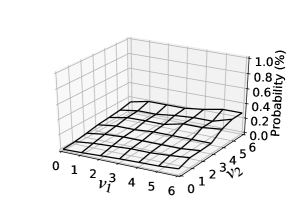
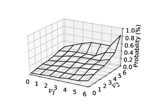
Fig. 5 shows item-choice probabilities estimated by our PV sequence model using the full-sample training set, where the PV sequence setting is $(n,m)=(5,6)$. Here, we focus on PV sequences in the form $\bm{v}=(v_{1},v_{2},v_{3},0,0)\in\Gamma$ and depict estimates of item-choice probabilities on $(v_{1},v_{2})\in[0,m]\times[0,m]$ for each $v_{3}\in\{0,1,2\}$. Note also that the number of associated user–item pairs decreased as the value of $v_{3}$ increased.

Because SeqEmp does not consider the monotonicity constraint (15), item-choice probabilities estimated by SeqEmp have irregular shapes for $v_{3}\in\{1,2\}$. In contrast, item-choice probabilities estimated with the monotonicity constraint (15) are relatively smooth. Because of the Up operation, item-choice probabilities estimated by SeqUM and SeqUS increase as $(v_{1},v_{2})$ moves from $(0,0)$ to $(6,6)$. Because of the Move operation, item-choice probabilities estimated by SeqUM also increase as $(v_{1},v_{2})$ moves from $(0,6)$ to $(6,0)$. Item-choice probabilities estimated by SeqUS are relatively high around $(v_{1},v_{2})=(3,3)$. This highlights the difference in the monotonicity constraint (15) between posets $(\Gamma,\preceq_{\texttt{UM}})$ and $(\Gamma,\preceq_{\texttt{US}})$.

Fig. 6 shows item-choice probabilities estimated by our PV sequence model using the 10%-sampled training set, where the PV sequence setting is $(n,m)=(5,6)$. Since the sample size was reduced in this case, item-choice probabilities estimated by SeqEmp are highly unstable. In particular, item-choice probabilities were estimated to be zero for all $(v_{1},v_{2})$ with $v_{1}\geq 3$ in Fig. 6(c), but this is unreasonable from the perspective of frequency. In contrast, SeqUM and SeqUS estimated item-choice probabilities that increase monotonically with respect to $(v_{1},v_{2})$.

References

- [1] C. C. Aggarwal, Recommender systems, Cham: Springer International Publishing, 2016
- [2] A. V. Aho, M. R. Garey, and J. D. Ullman, “The transitive reduction of a directed graph,” SIAM J. Comput., vol. 1, no. 2, pp. 131–137, 1972.
- [3] Y. Aıt-Sahalia and J. Duarte, “Nonparametric option pricing under shape restrictions,” J. Econom., vol. 116, no. 1–2, pp. 9–47, 2003.
- [4] E. E. Altendorf, A. C. Restificar, and T. G. Dietterich, “Learning from sparse data by exploiting monotonicity constraints,” in Proc. UAI, 2005, pp. 18–26.
- [5] A. Baumann, J. Haupt, F. Gebert, and S. Lessmann, “Changing perspectives: Using graph metrics to predict purchase probabilities,” Expert Syst. Appl., vol. 94, pp. 137–148, 2018.
- [6] J. Borges and M. Levene, “Evaluating variable-length markov chain models for analysis of user web navigation sessions,” IEEE Trans. Knowl. Data Eng., vol. 19, no. 4, pp. 441–452, 2007.
- [7] R. E. Bucklin and C. Sismeiro, “Click here for Internet insight: Advances in clickstream data analysis in marketing,” J. Interact. Mark., vol. 23, no. 1, pp. 35–48, 2009.
- [8] S. Chatterjee, A. Guntuboyina, and B. Sen, “On risk bounds in isotonic and other shape restricted regression problems,” Ann. Stat., vol. 43, no. 4, pp. 1774–1800, 2015.
- [9] Y. L. Chen, M. H. Kuo, S. Y. Wu, and K. Tang, “Discovering recency, frequency, and monetary (RFM) sequential patterns from customers’ purchasing data,” Electron. Commer. Res. Appl., vol. 8, no. 5, pp. 241–251, 2009.
- [10] D. Cirqueira, M. Hofer, D. Nedbal, M. Helfert, and M. Bezbradica, “Customer Purchase Behavior Prediction in E-commerce: Current Tasks, Applications and Methodologies,” in Inter. Workshop NFMCP, 2019.
- [11] T. H. Cormen, C. E. Leiserson, R. L. Rivest, and C. Stein, Introduction to algorithms, MIT press, 2009.
- [12] Y. Dong and W. Jiang, “Brand purchase prediction based on time-evolving user behaviors in e-commerce,” Concurr. Comput., vol. 31, no. 1, pp. e4882, 2019.
- [13] P. S. Fader, B. G. Hardie, and K. L. Lee, “RFM and CLV: Using iso-value curves for customer base analysis,” J. Mark. Res., vol. 42, no. 4, pp. 415–430, 2005.
- [14] B. R. Gaines, J. Kim, and H. Zhou, “Algorithms for fitting the constrained lasso,” J. Comput. Graph. Stat., vol. 27, no. 4, pp. 861–871, 2018.
- [15] P. Groeneboom and G. Jongbloed, Nonparametric estimation under shape constraints (Vol. 38), Cambridge University Press, 2014.
- [16] A. Guntuboyina and B. Sen, “Nonparametric shape-restricted regression,” Stat. Sci., vol. 33, no. 4, pp. 568–594, 2018.
- [17] Q. Han, T. Wang, S. Chatterjee, and R. J. Samworth, “Isotonic regression in general dimensions,” Ann. Stat., vol. 47, no. 5, pp. 2440–2471, 2019.
- [18] T. Huang and J. A. Van Mieghem, “Clickstream data and inventory management: Model and empirical analysis,” Prod. Oper. Manag., vol. 23, no. 3, pp. 333–347, 2014.
- [19] J. Iwanaga, N. Nishimura, N. Sukegawa, and Y. Takano, “Estimating product-choice probabilities from recency and frequency of page views,” Knowl. Based Syst., vol. 99, pp. 157–167, 2016.
- [20] J. Iwanaga, N. Nishimura, N. Sukegawa, and Y. Takano, “Improving collaborative filtering recommendations by estimating user preferences from clickstream data,” Electron. Commer. Res. Appl., vol. 37, 100877, 2019.
- [21] D. Jannach, M. Ludewig, and L. Lerche, “Session-based item recommendation in e-commerce: on short-term intents, reminders, trends and discounts,” User Model. User-adapt. Interact., vol. 27, no. 3–5, pp. 351–392, 2017.
- [22] P. K. Kannan, “Digital marketing: A framework, review and research agenda,” Int. J. Res. Mark., vol. 34, no. 1, pp. 22–45, 2017.
- [23] D. Koehn, S. Lessmann, and M. Schaal, “Predicting online shopping behaviour from clickstream data using deep learning,” Expert Syst. Appl., vol. 150, no. 15, 113342, 2020.
- [24] F. Le Gall, “Powers of tensors and fast matrix multiplication,” in Proc. ISSAC, 2014, pp. 296–303, 2014.
- [25] Q. Li, M. Gu, K. Zhou, and X. Sun, “Multi-Classes Feature Engineering with Sliding Window for Purchase Prediction in Mobile Commerce,” in IEEE ICDM Workshop, 2015, pp. 1048–1054.
- [26] D. Li, G. Zhao, Z. Wang, W. Ma, and Y. Liu, “A method of purchase prediction based on user behavior log,” in IEEE ICDM Workshop, 2015, pp. 1031–1039.
- [27] M. Ludewig and D. Jannach, “Evaluation of session-based recommendation algorithms,” User Model. User-adapt. Interact., vol. 28, no. 4–5, pp. 331–390, 2018.
- [28] R. L. Matzkin, “Semiparametric estimation of monotone and concave utility functions for polychotomous choice models,” Econometrica, vol. 59, no. 5, pp. 1315–1327, 1991.
- [29] W. W. Moe, “An empirical two-stage choice model with varying decision rules applied to internet clickstream data,” J. Mark. Res., vol. 43, no. 4, pp. 680–692, 2006.
- [30] W. W. Moe and P. S. Fader, “Dynamic conversion behavior at e-commerce sites,” Manage. Sci., vol. 50, no. 3, pp. 326–335, 2004.
- [31] A. L. Montgomery, S. Li, K. Srinivasan, and J. C. Liechty, “Modeling online browsing and path analysis using clickstream data,” Mark. Sci., vol. 23, no. 4, pp. 579–595, 2004.
- [32] N. Nishimura, N. Sukegawa, Y. Takano, and J. Iwanaga, “A latent-class model for estimating product-choice probabilities from clickstream data,” Inf. Sci., vol. 429,pp. 406–420, 2018.
- [33] E. W. Ngai, L. Xiu, and D. C. Chau, “Application of data mining techniques in customer relationship management: A literature review and classification,” Expert Syst. Appl., vol. 36, no. 2, pp. 2592–2602, 2009.
- [34] P. Orzechowski, W. La Cava, and J. H. Moore, “Where are we now? A large benchmark study of recent symbolic regression methods,” in Proc. GECCO, 2018, pp. 1183–1190.
- [35] P. M. Pardalos and G. Xue, “Algorithms for a class of isotonic regression problems,” Algorithmica, vol. 23, no. 3, pp. 211–222, 1999.
- [36] C. H. Park and Y. H. Park, “Investigating purchase conversion by uncovering online visit patterns,” Mark. Sci., vol. 35, no. 6, pp. 894–914, 2016.
- [37] A. Pitman and M. Zanker, “Insights from applying sequential pattern mining to e-commerce click stream data,” in IEEE ICDM Workshop, 2010, pp. 967–975.
- [38] J. Qiu, Z. Lin, and Y. Li, “Predicting customer purchase behavior in the e-commerce context,” Electron. Commer. Res., vol. 15, no. 4, pp. 427–452, 2015.
- [39] P. Romov and E. Sokolov, “Recsys challenge 2015: ensemble learning with categorical features,” in Proc. Inter. ACM RecSys Challenge, 2015, pp. 1–4.
- [40] B. Schröder, Ordered Sets: An Introduction with Connections from Combinatorics to Topology, Birkhäuser, 2016.
- [41] C. Sismeiro and R. E. Bucklin, “Modeling purchase behavior at an e-commerce web site: A task-completion approach,” J. Mark. Res., vol. 41, no. 3, pp. 306–323, 2004.
- [42] B. Stellato, G. Banjac, P. Goulart, A. Bemporad, and S. Boyd, “OSQP: An operator splitting solver for quadratic programs,” Math. Program. Comput., in press.
- [43] Q. F. Stout, “Isotonic regression for multiple independent variables,” Algorithmica, vol. 71, no. 2, pp. 450–470, 2015.
- [44] R. J. Tibshirani, H. Hoefling, and R. Tibshirani, “Nearly-isotonic regression,” Technometrics, vol. 53, no. 1, pp. 54–61, 2011.
- [45] E. Turban, J. Outland, D. King, J. K. Lee, T. P. Liang, and D. C. Turban, Electronic Commerce 2018: A Managerial and Social Networks Perspective, Springer, 2017.
- [46] D. Van den Poel and W. Buckinx, “Predicting online-purchasing behaviour,” Eur. J. Oper. Res., vol. 166, no. 2, pp. 557–575, 2005.
- [47] A. Vieira, “Predicting online user behaviour using deep learning algorithms,” arXiv preprint arXiv:1511.06247, 2015.
- [48] J. Wang and S. K. Ghosh, “Shape restricted nonparametric regression with Bernstein polynomials,” Comput. Stat. Data Anal., vol. 56, no. 9, pp. 2729–2741, 2012.
- [49] S. Warshall, “A theorem on boolean matrices,” J. ACM, vol. 9, no. 1, pp. 11–12, 1962.
- [50] Z. Wu, B. H. Tan, R. Duan, Y. Liu, and R. S. Mong Goh, “Neural modeling of buying behaviour for e-commerce from clicking patterns,” in Proc. Inter. ACM RecSys Challenge, 2015, pp. 1–4.
- [51] J. Yeo, S. Kim, E. Koh, S. W. Hwang, and N. Lipka, “Predicting online purchase conversion for retargeting,” in Proc. ACM Inter. Conf. WSDM, 2017, pp. 591–600.
- [52] Z. Yi, D. Wang, K. Hu, and Q. Li, “Purchase behavior prediction in m-commerce with an optimized sampling methods,” in IEEE ICDMW, 2015, pp. 1085–1092.
- [53] Y. Zhang and M. Pennacchiotti, “Predicting purchase behaviors from social media,” in Proc. Inter. Conf. WWW, 2013, pp. 1521–1532.
- [54] Y. Zhao, L. Yao, and Y. Zhang, “Purchase prediction using Tmall-specific features,” Concurr. Comput., vol. 28, no. 14, pp. 3879–3894, 2016.