Pre-trained Mixed Integer Optimization through Multi-variable Cardinality Branching

Yanguang Chen [email protected] Shanghai University of Finance and Economics Wenzhi Gao [email protected] contribution Stanford University Dongdong Ge [email protected] Shanghai Jiaotong University Yinyu Ye [email protected] Stanford University

Abstract

In this paper, we propose a Pre-trained Mixed Integer Optimization framework (PreMIO) that accelerates online mixed integer program (MIP) solving with offline datasets and machine learning models. Our method is based on a data-driven multi-variable cardinality branching procedure that splits the MIP feasible region using hyperplanes chosen by the concentration inequalities. Unlike most previous ML+MIP approaches that either require complicated implementation or suffer from a lack of theoretical justification, our method is simple, flexible, provable and explainable. Numerical experiments on both classical OR benchmark datasets and real-life instances validate the efficiency of our proposed method.

1 Introduction

Mixed integer programming (MIP) [30, 36] is pervasive in revenue management [5], production planning [27], combinatorial optimization [37], energy management [38], and many other fields. Despite its wide applicability, MIPs are generally hard to solve: state-of-the-art MIP solvers [10, 17, 19, 26] heavily rely on heuristics to be usable in practice. Therefore, designing effective heuristics has long been an important topic for MIP solving.

Among various MIP applications, some of them exhibit strong online nature: on a regular basis, similar models are solved with different data parameters. For example, in energy management [38] and production planning [27], MIPs are solved usually on a daily basis. Although this online nature imposes restrictions on the solution time, it ensures the availability of offline datasets, which opens the way for data-driven machine learning approaches. In this aspect, many successful ML+MIP attempts [6, 42] have been made and encouraging results are reported. However, successful ML+MIP attempts often resort to complex modifications to the MIP branch-and-bound or cut generation procedure. These modifications require intricate implementation and cannot be applied to commercial solvers without access to their source code. Additionally, machine learning-based methods are often less explainable, making it challenging to tune hyperparameters.

In view of these issues, we propose PreMIO, a Pre-trained Mixed Integer Optimization framework for online MIPs. PreMIO relies on probabilistic output of binary (integer) variables and applies a simple multi-variable cardinality branching procedure that constructs branching hyperplanes

\textstyle\sum_{i\in\mathcal{S}}y_{i}\leq\xi\quad\text{and}\quad\sum_{i\in\mathcal{S}}y_{i}\geq\xi+1,\quad\{y_{i}\}\text{ binary}.

With statistical learning theory [35], we further propose an intuitive way to select hyperplane $\xi$ . Our method ends up being simple, explainable and compatible with almost all the machine learning models and MIP solvers.

Contribution. In this paper,

•

We propose PreMIO, an efficient approach to exploit offline datasets to accelerate online MIP solving. Different from traditional methods that require complicated implementation, our method is simple but efficient, and compatible with existing machine models and MIP solvers.
•

We apply statistical learning theory to theoretically justify PreMIO and provide an intuitive way to choose the hyperparameters. Our setup can be of independent interest for designing other data-driven ML+MIP heuristics. Computational results verify the efficiency of our method.

1.1 Related work

ML+MIP

Machine learning has been applied in many aspects of MIP solving [15] and we focus on the attempts that have direct relation with MIP solving. In [1, 21, 25], the authors use machine learning models to imitate the behavior of an expensive branching rule in MIP. [11] proposes a graph representation of MIP and predicts the binary solution using graph convolutional network. [11] propose to add a cut that upper-bounds the distance between prediction and the MIP solution but do not further analyze this method. [25] also adopts a graph representation of MIP to predict binary variables, and proposes to combine the prediction with MIP diving heuristic (neural diving). In [16], the authors propose to learn the branching variable selection policy during the branch-and-bound procedure. [23] adopts imitation learning to learn a good pruning policy for a nonlinear MIP application. Recently there is growing interest in using reinforcement learning to accelerate MIP solving [7, 31, 32, 39], and we refer to [6, 42] for a comprehensive survey of ML/RL+MIP attempts.

Multi-variable branching

In the MIP literature, multi-variable branching is a natural extension of single-variable branching [20, 12] and this idea proves useful for linear MIPs [14]. In [41] the authors perform a case study on multi-knapsack problems. In this paper we use “cardinality multi-variable branching” since our branching hyperplanes take form of cardinality constraints.

Learning to solve MIP

Though most MIP+ML studies are empirical, there exist works in statistical learning theory that study learnability of MIPs. In [2], the authors derive the generalization bound for learning hybrid branching rules that take convex combination of different score functions. In [3], the bound is further improved for the MIP branch and bound procedure. In the same line of work, [4] analyzes the learnability of mixed integer and Gomory cutting planes.

Pre-trained optimization

The idea of pre-training is widely adopted in language models [28], but this idea is less common for optimization. In a recent work [22] the authors propose to use offline datasets to accelerate online blackbox optimization. In this paper, pre-training means machine learning models can be trained on offline solves before online MIP solving takes place. In view of conventional definition, we can interpret MIP solving as a training a model to get coefficient (solution), so that PreMIO is way to use previously trained (solved) MIP coefficients (solutions) to accelerate the forthcoming MIP training (solving).

1.2 Outline of the paper

The paper is organized as follows. In Section 2, we introduce PreMIO as well as its underlying multi-variable cardinality branching procedure, giving a theoretical analysis of its behavior using statistical learning theory. In Section 3, we discuss the practical aspects when implementing PreMIO. Finally, in Section 4, we conduct numerical experiments on both synthetic and real-life MIP instances to demonstrate the practical efficiency of our method.

2 Pre-trained optimization with cardinality branching

In this section, we introduce PreMIO and analyze its key component: a data-driven multi-variable cardinality branching heuristic. Cardinality branching splits the feasible region by adding hyperplanes involving multiple variables, and PreMIO adjusts the intercept of the hyperplanes based on prior knowledge from machine learning models. To start with, we put some efforts into providing a formal setup of parametric MIPs, pre-trained models and MIP learning theory.

2.1 Problem description and pre-training

We restrict our attention to binary problems and suppose that the problem with binary variables fixed is tractable. Then a parametric MIP $\mathcal{P}(\xi)$ of $n$ binary variables is defined as follows.

\mathcal{P}(\xi):=\min_{\mathbf{x},\mathbf{y}\in\{0,1\}^{n}}\leavevmode\nobreak\ \leavevmode\nobreak\ c(\mathbf{x},\mathbf{y};\xi)\quad\text{subject to}\quad h(\mathbf{x},\mathbf{y};\xi)\leq\textbf{0}

(1)

where $(c,h,\xi)$ encapsulates the problem structure and data parameters. With the above formulation, any MIP can be summarized by $\mathcal{P}(\xi)$ . We are interested in solving a sequence of problems that differ only in a subset of the parameters. i.e., we absorb common parameters into $c$ , $h$ and a problem is fully determined by the varying parameter $\xi\sim\Xi$ . Given $\mathcal{P}(\xi)$ , we use $\mathbf{y}^{\star}(\xi)=(y_{1}^{\star}(\xi),\ldots,y_{n}^{\star}(\xi))$ to denote one of its optimal solutions. Due to online nature of the problem, assume we have in hand sufficient data parameters and corresponding solutions by 1). collecting offline solution data; 2). generating instances through simulation. We further assume a machine learning model captures the mapping from $\xi$ to $\mathbf{y}^{\star}(\xi)$ . In other words, we can “pre-train” machine learning models to provide approximate knowledge of $\mathbf{y}^{\star}(\xi)$ . And this approximate knowledge will be used to help accelerate MIP solving. We call this procedure “pre-training” for optimization, and it contains:

Components of PreMIO

P1:

A collection of offline datasets $\mathcal{S}=\{(\xi,\mathbf{y}^{\star}{(\xi)})\}$ coming from either history or simulation.
P2:

Machine learning model $\hat{\mathbf{y}}$ pre-trained on $\mathcal{S}$ .
P3:

A mechanism to make use of $\hat{\mathbf{y}}(\xi)$ to help MIP solving.

This methodology is widely applied, but most researches focus on P2 and rather limited efforts are spent on P3. This motivates us to concentrate on P3, which differentiates PreMIO from the previous ML+MIP attempts. In the next subsections, we show how a cardinality branching procedure provides a solution for P3. More specifically, after entailing $\hat{\mathbf{y}}(\xi)$ with randomness through statistical learning theory, we observe an interesting correspondence between concentration inequalities and branching hyperplanes in the cardinality branching method.

2.2 Learning to solve MIP with PreMIO

In this subsection, we discuss how a learning procedure from $\xi$ to $\mathbf{y}^{\star}$ properly finds its place in learning theory through a standard binary classification model. We make the following assumptions.

A1:

(i.i.d. distribution) The MIP instances are characterized by parameters drawn i.i.d. from some unknown distribution $\xi\sim\Xi$ .
A2:

(Binomial posterior estimate) Given $\xi\sim\Xi$ and any $j\in[n]$ , parametric MIP $\mathcal{P}(\xi)$ has one unique solution. In other words, $\mathbb{P}\{y^{\star}_{j}(\xi)=0|\xi\}=1-\mathbb{P}\{y^{\star}_{j}(\xi)=1|\xi\}\in\{0,1\}$ .

Remark 1.

A1 is standard in learning theory and A2 can be satisfied by perturbing $c(\mathbf{x},\mathbf{y},\xi)$ .

Next we define what is a classifier in the MIP context.

Definition 1.

(Classifiers for MIPs) For a given binary variable $j$ , a binary classifier $\hat{y}_{j}$ is a function that accepts $\xi$ and outputs a binary prediction $\hat{y}_{j}(\xi)\in\{0,1\}$ .

Using the language of learning theory, we are interested in finding some classifier among a set of classifiers $\mathcal{Y}_{j}$ . Due to A2, the best classifier $\hat{y}_{j}(\xi)$ is exactly the Bayesian classifier $\mathbb{P}\{y^{\star}_{j}(\xi)=1|\xi\}$ and a MIP solver is one of them. However, classifying by exactly solving a MIP is often too expensive. Hence it’s natural to consider some $\hat{y}_{j}$ from a set of “inexpensive” classifiers $\mathcal{Y}_{j}$ . One choice of $\mathcal{Y}_{j}$ is parametric neural network, and $\mathcal{Y}_{j}$ can be interpreted as a set of neural networks of some given structure.

The last step is to find a good classifier from $\mathcal{Y}_{j}$ . Since it’s generally only possible for us to know the underlying distribution $\Xi$ through past data $\{\xi_{1},\ldots,\xi_{m}\}$ , we often resort to empirical risk minimization. Specifically, we consider 0-1 loss ERM classifier.

Definition 2.

(ERM classifier) Given binary variable $j$ a set of MIPs $\{\mathcal{P}(\xi_{1}),\ldots,\mathcal{P}(\xi_{m})\}$ the 0-1 loss ERM minimizer $\hat{y}_{j}=\hat{y}_{j}(\xi_{1},\ldots,\xi_{m})$ and ERM loss are respectively

\displaystyle\hat{y}_{j}

\displaystyle:=\underset{y_{j}\in\mathcal{Y}_{j}}{\arg\min}\big{\{}\textstyle\frac{1}{m}\sum_{i=1}^{m}\mathbb{I}\{y_{j}(\xi_{i})\neq y^{\star}_{j}(\xi_{i})\}\big{\}},\quad e_{j}:=\min_{y_{j}\in\mathcal{Y}_{j}}\big{\{}\frac{1}{m}\sum_{i=1}^{m}\mathbb{I}\{y_{j}(\xi_{i})\neq y^{\star}_{j}(\xi_{i})\}\big{\}}

Remark 2.

We adopt 0-1 loss for brevity. In practice we can employ a convex surrogate loss function [29] that makes training more tractable.

Now we have set up the ingredients to describe the MIP learning procedure: we collect offline $\{\mathcal{P}(\xi_{1}),\ldots,\mathcal{P}(\xi_{m})\}$ and their solutions, specify a set of classifiers $\mathcal{Y}_{j}$ and identify the best one in the sense of empirical risk. Then given a new instance $\mathcal{P}(\xi)$ , $\hat{y}_{j}(\xi)$ is used to predict $y_{j}^{\star}(\xi)$ .
The last component is to derive the generalization performance, i.e., how well $\hat{y}_{j}(\xi)$ works on $\mathcal{P}(\xi)$ . The following lemma gives what we want using VC-dimension.

Lemma 1 (VC dimension [34]).

Under A1 and A2, letting $\hat{y}_{j}$ be the ERM classifier under 0-1 loss and $e_{j}$ be the ERM loss, then with probability $1-\delta$ ,

\mathbb{P}_{\xi\sim\Xi}\{\hat{y}_{j}(\xi)\neq y^{\star}_{j}(\xi)\}\leq e_{j}+\sqrt{\tfrac{1}{m}\big{(}\operatorname{vc}(\mathcal{Y}_{j})\big{(}\log\tfrac{2m}{\operatorname{vc}(\mathcal{Y}_{j})}+1\big{)}+\log\tfrac{4}{\delta}\big{)}},

where $\operatorname{vc}(\mathcal{Y}_{j})$ is the VC dimension of $\mathcal{Y}_{j}$ .

Remark 3.

Lemma 1 is well-known in learning theory, and it shows a trade-off between $e_{j}$ and $\operatorname{vc}(\mathcal{Y}_{j})$ . This is intuitive in that complicated models of large VC-dimension generally fit better on offline data and give smaller ERM error.

Now that we have set up the background of learning theory for MIPs, we are ready to discuss how this result fits into a cardinality branching framework.

2.3 Learning and multi-variable cardinality branching

We now discuss how the theory of MIP learning can be exploited to accelerate actual MIP solving through a probabilistic cardinality branching procedure. Assume that we have $\hat{\mathbf{y}}=(\hat{y}_{1},\ldots,\hat{y}_{n})$ , and we suppose the following assumptions are true.

A3:

(Independent error rates) The events $\{\hat{y}_{j}(\xi)=y^{\star}_{j}(\xi)\}$ are independent.

A4:

(Learnability) We choose $\delta$ such that for each $j\in[n]$ ,

\Delta_{j}^{\delta}:=1-e_{j}-\sqrt{\tfrac{1}{m}\big{(}\operatorname{vc}(\mathcal{Y}_{j})\big{(}\log\tfrac{2m}{\operatorname{vc}(\mathcal{Y}_{j})}+1\big{)}+\log\tfrac{4}{\delta}\big{)}}>0.

Remark 4.

A3 is often used in ensemble methods in machine learning [13]. This can be fulfilled if $\{\hat{y}_{j}\}$ are trained on independent datasets. A4 states the learning model is non-trivial.

One way to make use of $\{\hat{y}_{j}(\xi)\}$ is through a variable fixing strategy. i.e., we choose a subset of the variables $\mathcal{J}\subseteq[n]$ and add the following constraints

y_{j}=\hat{y}_{j}(\xi),j\in\mathcal{J}.

Although convenient, it is unlikely that we can do this “safely”, as shown by the following theorem.

Theorem 1.

Given a set of variable fixing constraints $\{y_{j}=\hat{y}_{j}(\xi),j\in\mathcal{J}\}$ ,

\textstyle\mathbb{P}\{\hat{y}_{j}(\xi)=y_{j}^{\star}(\xi),j\in\mathcal{J}\}\geq(1-\delta)^{|\mathcal{J}|}\prod_{j\in\mathcal{J}}\Delta_{j}^{\delta},

where probability is taken over both training samples and $\xi\sim\Xi$ .

When $|\mathcal{J}|$ grows, the lower bound on $\mathbb{P}\{\hat{y}_{j}(\xi)=y_{j}^{\star}(\xi),j\in\mathcal{J}\}$ drops to 0 exponentially fast and this implies the traditional variable fixing method are less reliable. To alleviate this, a natural idea is to do risk pooling. In other words, we can place the “risky” binary predictions together to reduce the overall chance of making mistakes. More specifically, we define $\mathcal{U}:=\{j:\hat{y}_{j}(\xi)=1\},\mathcal{L}:=\{j:\hat{y}_{j}(\xi)=0\}$ according to their values and construct two hyperplanes

\mathcal{C}_{\mathcal{U}}:\textstyle\sum_{j\in\mathcal{U}}y_{j}\geq\zeta_{1}\quad\text{and}\quad\mathcal{C}_{\mathcal{L}}:\sum_{j\in\mathcal{L}}y_{j}\leq\zeta_{2}

(2)

Similar to single variable branching, these two hyperplanes (and their complement $\bar{\mathcal{C}}_{\mathcal{U}},\bar{\mathcal{C}}_{\mathcal{L}}$ ) divide the whole feasible region into four disjoint regions $\mathcal{P}_{\mathcal{C}_{\mathcal{U}},\mathcal{C}_{\mathcal{L}}},\mathcal{P}_{\mathcal{C}_{\mathcal{U}},\bar{\mathcal{C}}_{\mathcal{L}}},\mathcal{P}_{\bar{\mathcal{C}}_{\mathcal{U}},\mathcal{C}_{\mathcal{L}}},\mathcal{P}_{\bar{\mathcal{C}}_{\mathcal{U}},\bar{\mathcal{C}}_{\mathcal{L}}}$ , and we call this procedure “multi-variable cardinality branching”. However, compared to multi-variable branching in MIP literature, learning theory establishes a connection between $\{\hat{y}_{j}(\xi)\}$ and random variables. Applying concentration inequalities to $\{\hat{y}_{j}(\xi)\}$ , there is more to say about the choice of $\zeta_{1},\zeta_{2}$ as well as the behavior of these four regions. This leads to the following theorem.

Algorithm 1 PreMIO through multi-variable cardinality branching

1: input: MIP data parameter

(\xi)

, pre-trained MIP classifiers

\{\hat{y}_{j}\}

2: begin compute

\hat{\mathbf{y}}(\xi)

and let

\mathcal{U}=\{i:\hat{y}_{i}=1\},\mathcal{L}=\{i:\hat{y}_{i}=0\}

generate

\mathcal{C}_{\mathcal{U}},\mathcal{C}_{\mathcal{L}},\bar{\mathcal{C}}_{\mathcal{U}},\bar{\mathcal{C}}_{\mathcal{L}}

and four subproblems

\{\mathcal{P}_{\mathcal{C}_{\mathcal{U}},\mathcal{C}_{\mathcal{L}}},\mathcal{P}_{\mathcal{C}_{\mathcal{U}},\bar{\mathcal{C}}_{\mathcal{L}}},\mathcal{P}_{\bar{\mathcal{C}}_{\mathcal{U}},\mathcal{C}_{\mathcal{L}}},\mathcal{P}_{\bar{\mathcal{C}}_{\mathcal{U}},\bar{\mathcal{C}}_{\mathcal{L}}}\}

solve

\mathcal{P}_{\mathcal{C}_{\mathcal{U}},\mathcal{C}_{\mathcal{L}}},\mathcal{P}_{\mathcal{C}_{\mathcal{U}},\bar{\mathcal{C}}_{\mathcal{L}}},\mathcal{P}_{\bar{\mathcal{C}}_{\mathcal{U}},\mathcal{C}_{\mathcal{L}}},\mathcal{P}_{\bar{\mathcal{C}}_{\mathcal{U}},\bar{\mathcal{C}}_{\mathcal{L}}}

and get

\mathbf{y}^{\star}_{\mathcal{C}_{\mathcal{U}},\mathcal{C}_{\mathcal{L}}},\mathbf{y}^{\star}_{\mathcal{C}_{\mathcal{U}},\bar{\mathcal{C}}_{\mathcal{L}}},\mathbf{y}^{\star}_{\bar{\mathcal{C}}_{\mathcal{U}},\mathcal{C}_{\mathcal{L}}},\mathbf{y}^{\star}_{\bar{\mathcal{C}}_{\mathcal{U}},\bar{\mathcal{C}}_{\mathcal{L}}}

3: end output the best solution among

\big{\{}\mathbf{y}^{\star}_{\mathcal{C}_{\mathcal{U}},\mathcal{C}_{\mathcal{L}}},\mathbf{y}^{\star}_{\mathcal{C}_{\mathcal{U}},\bar{\mathcal{C}}_{\mathcal{L}}},\mathbf{y}^{\star}_{\bar{\mathcal{C}}_{\mathcal{U}},\mathcal{C}_{\mathcal{L}}},\mathbf{y}^{\star}_{\bar{\mathcal{C}}_{\mathcal{U}},\bar{\mathcal{C}}_{\mathcal{L}}}\big{\}}

Theorem 2.

Under all the assumptions of Lemma 1 and A3, A4, given a new MIP instance $\mathcal{P}(\xi),\xi\sim\Xi$ , letting $\mathcal{U}=\{j:\hat{y}_{j}(\xi)=1\}$ and $\mathcal{L}=\{j:\hat{y}_{j}(\xi)=0\}$ , we have

\textstyle\mathbb{P}\Big{\{}\sum_{j\in\mathcal{U}}y_{j}^{\star}(\xi)\geq(1-\delta)\sum_{j\in\mathcal{U}}\Delta_{j}^{\delta}-\gamma\Big{\}}\geq 1-\exp\big{(}-\frac{2\gamma^{2}}{|\mathcal{U}|}\big{)}

\textstyle\mathbb{P}\big{\{}\sum_{j\in\mathcal{L}}y_{j}^{\star}(\xi)\leq|\mathcal{L}|-(1-\delta)\sum_{j\in\mathcal{L}}\Delta_{j}^{\delta}+\gamma\big{\}}\geq 1-\exp\big{(}-\frac{2\gamma^{2}}{|\mathcal{L}|}\big{)}

for any $\gamma\geq 0$ , where probability is taken over all the training samples and $\xi\sim\Xi$ .

Through adjusting the hyperplanes intercepts using learning theory, PreMIO ensures the optimal solution lies in $\mathcal{P}_{\mathcal{C}_{\mathcal{U}},\mathcal{C}_{\mathcal{L}}}$ (the region defined by $\mathcal{C}_{\mathcal{U}}$ and $\mathcal{C}_{\mathcal{L}}$ ) with high probability. Although Theorem 2 mainly serves as a theoretical result, it provides intuition and theoretical justification of our method.

Remark 5.

One advantage of Algorithm 1 is that we can often restrict our computation to the first subproblem when 1). we have high confidence that $\mathcal{P}_{\mathcal{C}_{\mathcal{U}},\mathcal{C}_{\mathcal{L}}}$ contains the optimal solution or 2). $\mathcal{P}_{\mathcal{C}_{\mathcal{U}},\mathcal{C}_{\mathcal{L}}}$ already outputs a satisfying solution. And in the worst case we solve the four subproblems without any loss of optimality.

In the next section, we conclude with several practical aspects of PreMIO. Since we do not necessarily need the assumptions in real applications, there is more freedom to exploit the probabilistic interpretation of binary predictions and the concentration bound.

3 Practical aspects of PreMIO

In this section, we discuss several practical aspects of PreMIO and make it more realistic. We discard the previous assumptions and reinterpret $\hat{y}_{j}(\xi)$ as its most natural counterpart in practice, conditional probability: we consider $\hat{y}_{j}(\xi)$ as $\hat{y}_{j}(\xi)=\mathbb{E}[y_{i}^{\star}(\xi)|\xi]=\mathbb{E}[\mathbb{I}\{y_{i}^{\star}(\xi)=1\}|\xi]=\mathbb{P}\{y_{i}^{\star}(\xi)=1|\xi\}.$

A5:

(Conditional expectation) $\hat{y}_{j}(\xi)$ represents the conditional expectation $\mathbb{E}[y_{i}^{\star}(\xi)|\xi]$ .
A6:

(Independent output) $\{\hat{y}_{j}(\xi)\}$ are conditionally independent given $\xi$ .

Remark 6.

Given A1 and A5, A6 holds naturally if we train over disjoint datasets; In general A5 almost never holds since we cannot expect a machine learning model to capture the posterior based on finite offline data. However, these assumptions are sufficient to provide an intuitive heuristic and guide our choice of hyperparameters.

3.1 Practical probabilistic multi-variable cardinality branching

After we redefine $\hat{y}_{j}(\xi)$ , it is possible to give a cleaner version of Theorem 2.

Theorem 3.

Under A1, A5 and A6, given independent random variables $y_{1}^{\star}(\xi),\ldots,y_{n}^{\star}(\xi)$ such that $\mathbb{E}[y_{i}^{\star}(\xi)|\xi]=\hat{y}_{i}(\xi)$ , letting $\mathcal{U}:=\{i:\hat{y}_{i}(\xi)\geq\tau\}$ and $\mathcal{L}=\{i:\hat{y}_{i}(\xi)<1-\tau\}$ for $0.5\leq\tau\leq 1$ . Then with probability at least $1-\delta$ , each of the inequalities below holds.

	$\displaystyle\mathcal{C}_{\mathcal{U}}:$	$\displaystyle\textstyle\sum_{i\in\mathcal{U}}y_{i}^{\star}(\xi)\geq\sum_{i\in\mathcal{U}}\hat{y}_{i}(\xi)-\sqrt{\tfrac{\|\mathcal{U}\|}{2}\log(1/\delta)}\geq\tau\|\mathcal{U}\|-\sqrt{\tfrac{\|\mathcal{U}\|}{2}\log(1/\delta)}$
	$\displaystyle\mathcal{C}_{\mathcal{L}}:$	$\displaystyle\textstyle\sum_{i\in\mathcal{L}}y_{i}^{\star}(\xi)\leq\sum_{i\in\mathcal{L}}\hat{y}_{i}(\xi)+\sqrt{\tfrac{\|\mathcal{L}\|}{2}\log(1/\delta)}\leq(1-\tau)\|\mathcal{L}\|+\sqrt{\tfrac{\|\mathcal{L}\|}{2}\log(1/\delta)}$

Theorem 3 essentially shows a natural hyperparameter tuning strategy. And as we mentioned in Remark 5, PreMIO can be flexibly implemented. First, for many industrial applications, it is often unnecessary to solve all the four subproblems, and we can stop whenever we get a satisfying solution; even for scenarios where accurate solution and certificate both are required, we can solve the four subproblems in parallel with objective pruning. We elaborate more on pruning in Section 3.2. Besides, though it is common to branch at root node, PreMIO can be implemented at any node in a branch-and-bound search tree through advanced solver interfaces. Last, one advantage of PreMIO lies in its low dependence on the problem structure, and thus high compatibility. Whenever $\hat{y}_{j}$ is available, PreMIO is applicable almost with no extra efforts. We believe that PreMIO can be further enhanced along with the development of learning theory.

3.2 Efficient pruning using objective cuts

When PreMIO is applied to solve MIP exactly, it is necessary to solve all four subproblems to certify optimality. However, prior knowledge that optimal solution more likely lies in $\mathcal{P}_{\mathcal{C}_{\mathcal{U}},\mathcal{C}_{\mathcal{L}}}$ accelerates the solution procedure. Denote $c^{\star}(\{\mathcal{C}_{k}\})$ to be the optimal value of MIP with extra constraints $\{\mathcal{C}_{k}\}$ . Suppose we solve $\mathcal{P}_{\mathcal{C}_{\mathcal{U}},\mathcal{C}_{\mathcal{L}}}$ and get the optimal objective $c^{\star}_{\mathcal{U},\mathcal{L}}:=c^{\star}(\{\mathcal{C}_{\mathcal{U}},\mathcal{C}_{\mathcal{L}},\})$ . Then we add constraint $c\leq c^{\star}_{\mathcal{U},\mathcal{L}}$ to $\mathcal{P}_{\mathcal{C}_{\bar{\mathcal{U}}},\mathcal{C}_{\mathcal{L}}}$ , $\mathcal{P}_{\mathcal{C}_{\mathcal{U}},\mathcal{C}_{\bar{\mathcal{L}}}}$ and $\mathcal{P}_{\mathcal{C}_{\bar{\mathcal{U}}},\mathcal{C}_{\bar{\mathcal{L}}}}$ and solve

\displaystyle c^{\star}_{\bar{\mathcal{U}},\mathcal{L}}

\displaystyle=c^{\star}(\{\mathcal{C}_{\bar{\mathcal{U}}},\mathcal{C}_{\mathcal{L}},c\leq c^{\star}_{\mathcal{U},\mathcal{L}}\}),\leavevmode\nobreak\ c^{\star}_{\mathcal{U},\bar{\mathcal{L}}}=c^{\star}(\{\mathcal{C}_{\mathcal{U}},\mathcal{C}_{\bar{\mathcal{L}}},c\leq c^{\star}_{\mathcal{U},\mathcal{L}}\}),\leavevmode\nobreak\ c^{\star}_{\bar{\mathcal{U}},\bar{\mathcal{L}}}=c^{\star}(\{\mathcal{C}_{\bar{\mathcal{U}}},\mathcal{C}_{\bar{\mathcal{L}}},c\leq c^{\star}_{\mathcal{U},\mathcal{L}}\}).

So long as $\mathcal{P}_{\mathcal{C}_{\mathcal{U}},\mathcal{C}_{\mathcal{L}}}$ excludes all the optimal solutions to MIP, $c^{\star}_{\bar{\mathcal{U}},\mathcal{L}}=c^{\star}_{\mathcal{U},\bar{\mathcal{L}}}=c^{\star}_{\bar{\mathcal{U}},\bar{\mathcal{L}}}=+\infty$ and other branches can be pruned efficiently, often at the cost of solving three LP relaxations.

3.3 Data-free PreMIO using interior point solution

Despite being a data-driven method, the idea behind PreMIO is applicable so long as a reasonable likelihood estimate of binaries is available. In the MIP context, a natural surrogate is the optimal solution of root relaxation. Denote $\mathbf{y}^{\star}_{\operatorname{Root}}$ to be the MIP root relaxation solution after root cut loops, we can construct hyperplanes based on $\mathbf{y}^{\star}_{\operatorname{Root}}$ instead. In other words, we view LP solving as a machine learning algorithm. And it turns out interior point method ends up being an efficient “learning algorithm”.

4 Numerical Experiment

In this section, we conduct experiments to validate the performance of PreMIO .

4.1 Experiment setup

Hardware

Experiments run on Intel(R) Xeon(R) CPU [email protected] PC of 64GB memory.

MIP data

We use two combinatorial problems 1). Multi-knapsack problem (MKP). 2). Set covering problem (SCP) and a real-life problem 3). Security-constrained unit commitment (SCUC) from IEEE 118 as our testing models. We use 4). MIPLIB collection from [18] to test data-free PreMIO.

•

For MKP models $\max_{\mathbf{Ay}\leq\mathbf{b},\mathbf{y}\in\{0,1\}^{n}}\langle\mathbf{c},\mathbf{y}\rangle$ , $\mathbf{A}\in\mathbb{R}^{m\times n}$ , we generate synthetic datasets according to the problem setup in [9]. After choosing problem sizes $(m,n)\in\{(10,250),(10,500),(30,250),(30,500)\}$ , each element of $a_{ij}$ is uniformly drawn from $\{1,\ldots,1000\}$ and $c_{i}=\frac{1}{m}\sum_{i}a_{ij}+\delta_{i}$ where $\delta_{i}$ is sampled from $\{1,\ldots,500\}$ . Then for each setup we fix $\mathbf{A},\mathbf{c}$ and generate $500$ i.i.d. instances with $b_{i}\sim\mathcal{U}[0.8\cdot\frac{1}{4n}\sum_{j}a_{ij},1.2\cdot\frac{1}{4n}\sum_{j}a_{ij}]$ for training. We generate 20 new instances for testing. In MKP $\xi=\mathbf{b}$ .
•

For SCP models $\min_{\mathbf{Ay}\geq\textbf{1},\mathbf{y}\in\{0,1\}^{n}}\langle\mathbf{c},\mathbf{y}\rangle,\mathbf{A}\in\mathbb{R}^{m\times n}$ , we use dataset from [33]. After choosing problem sizes $(m,n)\in\{(1000,10000),(1000,20000),(2000,20000)\}$ and generating $\mathbf{A}$ with sparsity 0.01, $\bar{c}_{i}\in\{1,\ldots,100\}$ , for each setup we fix $\mathbf{A}$ and generate $500$ i.i.d. instances with $c_{i}\sim\mathcal{U}[0.8\cdot\bar{c}_{i},1.2\cdot\bar{c}_{i}]$ for training. We generate 20 new instances for testing. In SCP $\xi=\mathbf{c}$ .
•

For SCUC models $\min_{(\mathbf{x},\mathbf{y}),h(\mathbf{x},\mathbf{y})\leq\textbf{0},\mathbf{Dx}=\mathbf{d}}c(\mathbf{x},\mathbf{y})$ , we use IEEE 118 dataset [8, 40] of time horizon 96, fix all the information of generators and simulate load demand vector $\mathbf{d}\in\mathcal{U}[l,u]^{96},(l,u)\in\{(3000,5000),(4000,6000)\}$ . For each setup we generate 200 i.i.d. instances for training and 5 new instances for testing. In SCUC $\xi=\mathbf{d}$ .
•

We take 132 instances from MIPLIB benchmark set [18].

Training data

Due to license limitations we apply CPLEX to build offline data $\{\xi,\mathbf{y}^{\star}(\xi)\}$ . Each MKP is given 300 seconds and solved to a $10^{-4}$ relative gap; Each SCP of size $(m,n)=(1000,10000)$ is given 300 seconds and solved to $10^{-3}$ gap; Each SCP of size $(m,n)\in\{(1000,20000),(2000,20000)\}$ is given 600 seconds and solved to a $10^{-1}$ gap; Each SCUC is given 3600 seconds and solved to a $10^{-4}$ gap.

Learning model

We choose logistic regression model $y=\sigma(\beta_{0}+\langle\beta,\xi\rangle)=\frac{1}{1+\exp(\beta_{0}+\langle\beta,\xi\rangle)}$ of low VC dimension $\mathcal{O}(\dim(\beta))$ as our learning model. For each binary variable, we use a separate regression model and train $\hat{y}_{i}$ over the whole training set. The probabilistic output $\sigma(\hat{\beta}_{0}+\langle\hat{\beta},\xi\rangle)$ is used for generating branching hyperplanes as mentioned by Section 3.

4.2 PreMIO as a primal heuristic

In this section, we benchmark performance of PreMIO as a primal heuristic.

Testing configurations and performance

We choose two current leading MIP solvers Gurobi and COPT from MIP benchmark [24] and use them to evaluate performance improvement using PreMIO to improve primal upperbound. Given a new MIP instance from our test set, we construct the two hyperplanes according to Theorem 3 and use hyperparameters $\delta=0.8,\tau=0.9$ . After generating the hyperplanes, we allow 120 seconds for the solver to solve $\mathcal{P}_{\mathcal{C}_{\mathcal{L}},\mathcal{C}_{\mathcal{U}}}$ and obtain the time $T_{\text{\text{{{{PreMIO}}}}}}$ it spends achieving the best objective value $F_{\text{\text{{{{PreMIO}}}}}}$ . Then we run the solver again, with a time limit of 3600 seconds, on the MIP instance without adding hyperplanes and record the time $T_{\text{\text{{{Original}}}}}$ for the solver to reach $F_{\text{\text{{{{PreMIO}}}}}}$ . We take shifted geometric mean (SGM) over testing instances and compute

	$\displaystyle\textstyle\bar{T}_{\text{\text{{{{PreMIO}}}}}}$	$\displaystyle:=\exp({\textstyle\frac{1}{n}\sum_{i=1}^{n}}\log\max\{1,T^{i}_{\text{\text{{{{PreMIO}}}}}}+10\})-10$
	$\displaystyle\textstyle\bar{T}_{\text{\text{{{Original}}}}}$	$\displaystyle:=\exp({\textstyle\frac{1}{n}\sum_{i=1}^{n}}\log\max\{1,T^{i}_{\text{\text{{{Original}}}}}+10\})-10$

We report average speedup $\Sigma:=\frac{\bar{T}_{\text{\text{{{Original}}}}}}{\bar{T}_{\text{\text{{{{PreMIO}}}}}}}$ as our performance evaluation metric. Finally, to see how our method interacts with the existing heuristics of MIP solvers, for each setup we adjust solvers’ heuristic-relevant parameters from low to high. Specifically we use L, M, H to represent Gurobi Heuristics parameter $\{0,0.05,1.0\}$ and COPT HeurLevel parameter $\{0,2,3\}$ , where L means turning off heuristics and H means using heuristics aggressively.

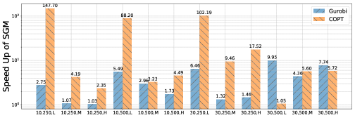
Refer to caption — Figure 1: From top to bottom: speedup on MKP, SCP and SCUC instances. Left: speedup of Gurobi, Right: speedup of COPT. Each tuple in the x-axis represents $(m,n,\text{Heuristic})$ and y-axis denotes average speedup $\Sigma$ in the corresponding settings.

As is illustrated by Figure 1, PreMIO achieves remarkable speedup on two commercial solvers when applied to both synthetic datasets and problems with real-life background. For MKP instances we observe speedup of $\geq 500\%$ for several settings and an average speedup of $\geq 50\%$ is obtained on SCUC problems. Particularly for SCP instances, we observe a consistent speedup among all testing instances, often exceeding 10 times. The speedup demonstrates the practical efficiency of our method. Beyond speedup in primal solution finding, we observe that the interaction between PreMIO and the internal heuristics is less predictable over different datasets and different solvers. For example, on SCP we see a clear trend of diminishing speedup for both solvers when the problem is relatively easy (small $(m,n)$ ). However, when the problem becomes more difficult ( $(m,n)=(2000,20000)$ ), PreMIO tends to bring about more speedup for COPT. The same instability of speedup is also observed on SCP and SCUC instances. This implies further space of improvement by tailoring the internal heuristics in the solver according to the specific application.

4.3 PreMIO as a branching rule

In this section, we apply PreMIO as an external branching rule. We implement the objective cut pruning strategy in Section 3.2 and the test Gurobi on knapsack instances with gap 0.015% and 0.01% for 20 instances. Gurobi runs under 4 threads and a time limit of 3600 seconds. The rest of the parameters remain unchanged.

Table 1: Time for 20 solves on MKP instances. Left:

(m,n)=(500,10)

; Right:

(m,n)=(500,30)

Instance	Original	PreMIO	Instance	Original	PreMIO	Instance	Original	PreMIO	Instance	Original	PreMIO
1	87.5	28.4	6	86.2	37.5	1	3600.0	2270.0	6	67.1	72.8
2	45.9	45.0	7	40.1	33.6	2	2883.0	2242.0	7	744.1	370.9
3	9.0	26.2	8	238.6	166.9	3	732.1	1111.5	8	2298.3	1540.6
4	7.5	6.0	9	45.8	43.6	4	315.0	302.3	9	3600.0	3600.0
5	10.6	10.8	10	9.2	24.8	5	3600.0	1779.7	10	2976.3	1575.1
SGM	28.7	25.8				SGM	1283	979

According to Table 1, we observe a 13%(20%) improvement on solution time. Moreover, as we discussed in Section 3.2, the three subproblems are pruned within one second and they are almost “free” to solve. This experiment reveals the efficiency of PreMIO even when the underlying solver is only accessible through a blackbox. The solution time improvement is not so impressive compared to when we employ PreMIO as a primal heuristic. However, we believe a 20% improvement over the state-of-the-art solvers is still non-trivial, taking into account its flexibility.

4.4 Data-free PreMIO for general MIP

Finally, we test the performance of PreMIO as a data-free primal heuristic for general MIP solving. We use the interior point solution of LP relaxation as the binary prediction surrogate and let COPT run under a time limit of 3600 seconds. The rest of the solver parameters remain unchanged. If 1). $\mathcal{P}_{\mathcal{C}_{\mathcal{U}},\mathcal{C}_{\mathcal{L}}}$ is certified as infeasible immediately or 2). both $\mathcal{P}_{\mathcal{C}_{\mathcal{U}},\mathcal{C}_{\mathcal{L}}}$ and the original problem exceed the time limit, PreMIO is considered not applicable and the instance is excluded. We end up getting 57 MIP instances. Table 2 and 3 summarize the SGM and detailed solution statistics.

Table 2: Shifted geometric mean for effective MIPLIB instances

Parameter	SGM compared to No PreMIO
$\delta=0.01,\tau=0.9$	$>1.0$
$\delta=10^{-8},\tau=0.9$	0.84
$\delta=10^{-15},\tau=0.9$ 5	0.94

Table 3: MIPLIB instances

\delta=10^{-8},\tau=0.9

f

denotes objective,

T

denotes solution time

Instance	$f_{\text{\text{{{PreMIO}}}}}$	$T_{\text{\text{{{PreMIO}}}}}$	$f_{\text{\text{{{Original}}}}}$	$T_{\text{\text{{{Original}}}}}$	Instance	$f_{\text{\text{{{PreMIO}}}}}$	$T_{\text{\text{{{PreMIO}}}}}$	$f_{\text{\text{{{Original}}}}}$	$T_{\text{\text{{{Original}}}}}$
academictables	0.0e+00	846.9	1.0e+00	3600.0	ci-s4	3.3e+03	121.4	3.3e+03	101.0
acc-tight5	0.0e+00	2.1	0.0e+00	4.2	blp-ic98	4.5e+03	156.2	4.5e+03	332.1
22433	2.1e+04	0.5	2.1e+04	0.7	brazil3	2.4e+02	70.7	2.4e+02	87.7
23588	8.1e+03	1.1	8.1e+03	0.9	comp08-2idx	3.7e+01	18.6	3.7e+01	16.2
30_70_45_05_100	9.0e+00	12.8	9.0e+00	13.6	cmflsp50-24-8-8	5.6e+07	2361.9	5.6e+07	2764.3
amaze22012-06-28i	0.0e+00	0.6	0.0e+00	0.3	diameterc-msts	7.3e+01	32.4	7.3e+01	30.7
arki001	7.5e+06	71.9	7.5e+06	84.2	comp07-2idx	6.0e+00	321.2	6.0e+00	468.8
assign1-5-8	2.1e+02	1317.3	2.1e+02	1306.9	aflow40b	1.2e+03	88.9	1.2e+03	121.0
a1c1s1	1.2e+04	204.1	1.2e+04	217.7	cap6000	-2.5e+06	0.6	-2.5e+06	0.3
blp-ar98	6.2e+03	293.6	6.2e+03	340.7	ab71-20-100	-1.0e+10	3.3	-1.0e+10	3.5
ab51-40-100	-1.0e+10	6.1	-1.0e+10	6.5	beavma	3.8e+05	0.2	3.8e+05	0.2
a2c1s1	1.1e+04	333.2	1.1e+04	352.5	cost266-UUE	2.5e+07	1549.1	2.5e+07	1574.1
blp-ar98	6.2e+03	293.6	6.2e+03	340.7	csched007	3.5e+02	383.2	3.5e+02	408.5
blp-ic97	4.0e+03	441.4	4.0e+03	465.4	csched008	1.7e+02	80.2	1.7e+02	255.3
aflow30a	1.2e+03	4.4	1.2e+03	4.5	danoint	6.6e+01	650.5	6.6e+01	484.3

According to Table 2 and 3, we observe an SGM improvement of up to 16% on the 57 instances. We also make the following comments:

•

Some instances (e.g., academictable) become solvable on the primal side when we solve $\mathcal{P}_{\mathcal{C}_{\mathcal{U}},\mathcal{C}_{\mathcal{L}}}$

We also observe that if $\mathcal{P}_{\mathcal{C}_{\mathcal{U}},\mathcal{C}_{\mathcal{L}}}$ is feasible, it hardly compromises optimality
•

It’s possible that $\mathcal{P}_{\mathcal{C}_{\mathcal{U}},\mathcal{C}_{\mathcal{L}}}$ is infeasible when LP solution is used. Especially if the LP relaxation is weak, the LP solution gives the wrong direction. In this case PreMIO should not be employed.
•

Very conservative PreMIO parameters are required. As Table 2 suggests, we need to take $\delta$ (the error parameter) very close to 0 to yield competitive performance, which is very different from the data-driven case (where we take $\delta$ up to 0.3 without incurring infeasibility).

As a data-independent heuristic, PreMIO also exhibits potential for general MIP solving.

5 Conclusions

In this paper, we propose PreMIO as a general framework for learning to solve online MIPs using pre-trained machine learning models. Leveraging statistical learning theory, we identify the correspondence between concentration inequalities and multi-variable branching hyperplanes and use this intuition to design a data-driven multi-variable branching procedure. PreMIO identifies a proper way to incorporate prior knowledge from offline solves into online MIP solving and is intuitive, explainable and flexible. Our setup, which establishes a connection between binary random variables and binary predictions, can be of independent interest to further data-driven MIP heuristic design.

References

[1] Alejandro Marcos Alvarez, Quentin Louveaux, and Louis Wehenkel. A machine learning-based approximation of strong branching. INFORMS Journal on Computing, 29:185–195, 2017.
[2] Maria-Florina Balcan, Travis Dick, Tuomas Sandholm, and Ellen Vitercik. Learning to branch. In International conference on machine learning, pages 344–353. PMLR, 2018.
[3] Maria-Florina Balcan, Siddharth Prasad, Tuomas Sandholm, and Ellen Vitercik. Improved sample complexity bounds for branch-and-cut. In 28th International Conference on Principles and Practice of Constraint Programming (CP 2022), 2022.
[4] Maria-Florina F Balcan, Siddharth Prasad, Tuomas Sandholm, and Ellen Vitercik. Structural analysis of branch-and-cut and the learnability of gomory mixed integer cuts. Advances in Neural Information Processing Systems, 35:33890–33903, 2022.
[5] Stefano Benati and Romeo Rizzi. A mixed integer linear programming formulation of the optimal mean/value-at-risk portfolio problem. European Journal of Operational Research, 176(1):423–434, 2007.
[6] Yoshua Bengio, Andrea Lodi, and Antoine Prouvost. Machine learning for combinatorial optimization: a methodological tour d’horizon. European Journal of Operational Research, 290(2):405–421, 2021.
[7] Timo Berthold and Gregor Hendel. Learning to scale mixed-integer programs. In Proceedings of the AAAI Conference on Artificial Intelligence, volume 35, pages 3661–3668, 2021.
[8] Adam B Birchfield, Ti Xu, Kathleen M Gegner, Komal S Shetye, and Thomas J Overbye. Grid structural characteristics as validation criteria for synthetic networks. IEEE Transactions on power systems, 32(4):3258–3265, 2016.
[9] Paul C Chu and John E Beasley. A genetic algorithm for the multidimensional knapsack problem. Journal of heuristics, 4:63–86, 1998.
[10] IBM ILOG Cplex. V12. 1: User’s manual for cplex. International Business Machines Corporation, 46(53):157, 2009.
[11] Jian-Ya Ding, Chao Zhang, Lei Shen, Shengyin Li, Bing Wang, Yinghui Xu, and Le Song. Accelerating primal solution findings for mixed integer programs based on solution prediction. In Proceedings of the aaai conference on artificial intelligence, volume 34, pages 1452–1459, 2020.
[12] Matteo Fischetti and Andrea Lodi. Local branching. Mathematical programming, 98:23–47, 2003.
[13] Yoav Freund and Robert E Schapire. A decision-theoretic generalization of on-line learning and an application to boosting. Journal of computer and system sciences, 55(1):119–139, 1997.
[14] Gerald Gamrath, Anna Melchiori, Timo Berthold, Ambros M Gleixner, and Domenico Salvagnin. Branching on multi-aggregated variables. In Integration of AI and OR Techniques in Constraint Programming: 12th International Conference, CPAIOR 2015, Barcelona, Spain, May 18-22, 2015, Proceedings 12, pages 141–156. Springer, 2015.
[15] Maxime Gasse, Simon Bowly, Quentin Cappart, Jonas Charfreitag, Laurent Charlin, Didier Chételat, Antonia Chmiela, Justin Dumouchelle, Ambros Gleixner, Aleksandr M Kazachkov, et al. The machine learning for combinatorial optimization competition (ml4co): Results and insights. In NeurIPS 2021 competitions and demonstrations track, pages 220–231. PMLR, 2022.
[16] Maxime Gasse, Didier Chételat, Nicola Ferroni, Laurent Charlin, and Andrea Lodi. Exact combinatorial optimization with graph convolutional neural networks. Advances in neural information processing systems, 32, 2019.
[17] Dongdong Ge, Qi Huangfu, Zizhuo Wang, Jian Wu, and Yinyu Ye. Cardinal optimizer (copt) user guide. arXiv preprint arXiv:2208.14314, 2022.
[18] Ambros Gleixner, Gregor Hendel, Gerald Gamrath, Tobias Achterberg, Michael Bastubbe, Timo Berthold, Philipp Christophel, Kati Jarck, Thorsten Koch, Jeff Linderoth, et al. Miplib 2017: data-driven compilation of the 6th mixed-integer programming library. Mathematical Programming Computation, 13(3):443–490, 2021.
[19] LLC Gurobi Optimization. Gurobi optimizer reference manual, 2021.
[20] Miroslav Karamanov and Gérard Cornuéjols. Branching on general disjunctions. Mathematical Programming, 128(1-2):403–436, 2011.
[21] Elias Khalil, Pierre Le Bodic, Le Song, George Nemhauser, and Bistra Dilkina. Learning to branch in mixed integer programming. In Proceedings of the AAAI Conference on Artificial Intelligence, volume 30, 2016.
[22] Siddarth Krishnamoorthy, Satvik Mehul Mashkaria, and Aditya Grover. Generative pretraining for black-box optimization. arXiv preprint arXiv:2206.10786, 2022.
[23] Mengyuan Lee, Guanding Yu, and Geoffrey Ye Li. Learning to branch: Accelerating resource allocation in wireless networks. IEEE Transactions on Vehicular Technology, 69(1):958–970, 2019.
[24] Hans D Mittelmann. Benchmarking optimization software-a (hi) story. In SN operations research forum, volume 1, page 2. Springer, 2020.
[25] Vinod Nair, Sergey Bartunov, Felix Gimeno, Ingrid Von Glehn, Pawel Lichocki, Ivan Lobov, Brendan O’Donoghue, Nicolas Sonnerat, Christian Tjandraatmadja, Pengming Wang, et al. Solving mixed integer programs using neural networks. arXiv preprint arXiv:2012.13349, 2020.
[26] FICO Xpress Optimizer. v8. 11 reference manual, 2021.
[27] Yves Pochet and Laurence A Wolsey. Production planning by mixed integer programming, volume 149. Springer, 2006.
[28] Alec Radford, Karthik Narasimhan, Tim Salimans, Ilya Sutskever, et al. Improving language understanding by generative pre-training. 2018.
[29] Mark D Reid and Robert C Williamson. Surrogate regret bounds for proper losses. In Proceedings of the 26th Annual International Conference on Machine Learning, pages 897–904, 2009.
[30] Nikolaos V Sahinidis. Mixed-integer nonlinear programming 2018, 2019.
[31] Lara Scavuzzo, Feng Chen, Didier Chételat, Maxime Gasse, Andrea Lodi, Neil Yorke-Smith, and Karen Aardal. Learning to branch with tree mdps. Advances in Neural Information Processing Systems, 35:18514–18526, 2022.
[32] Jialin Song, Yisong Yue, Bistra Dilkina, et al. A general large neighborhood search framework for solving integer linear programs. Advances in Neural Information Processing Systems, 33:20012–20023, 2020.
[33] Shunji Umetani. Exploiting variable associations to configure efficient local search algorithms in large-scale binary integer programs. European Journal of Operational Research, 263(1):72–81, 2017.
[34] Vladimir Vapnik, Esther Levin, and Yann Le Cun. Measuring the vc-dimension of a learning machine. Neural computation, 6(5):851–876, 1994.
[35] Roman Vershynin. High-dimensional probability: An introduction with applications in data science, volume 47. Cambridge university press, 2018.
[36] Laurence A Wolsey. Integer programming. John Wiley & Sons, 2020.
[37] Laurence A Wolsey and George L Nemhauser. Integer and combinatorial optimization, volume 55. John Wiley & Sons, 1999.
[38] Allen J Wood, Bruce F Wollenberg, and Gerald B Sheblé. Power generation, operation, and control. John Wiley & Sons, 2013.
[39] Yaoxin Wu, Wen Song, Zhiguang Cao, and Jie Zhang. Learning large neighborhood search policy for integer programming. Advances in Neural Information Processing Systems, 34:30075–30087, 2021.
[40] Ti Xu, Adam B Birchfield, Kathleen M Gegner, Komal S Shetye, and Thomas J Overbye. Application of large-scale synthetic power system models for energy economic studies. 2017.
[41] Yu Yang, Natashia Boland, and Martin Savelsbergh. Multivariable branching: A 0-1 knapsack problem case study. INFORMS Journal on Computing, 33(4):1354–1367, 2021.
[42] Jiayi Zhang, Chang Liu, Xijun Li, Hui-Ling Zhen, Mingxuan Yuan, Yawen Li, and Junchi Yan. A survey for solving mixed integer programming via machine learning. Neurocomputing, 519:205–217, 2023.

\doparttoc\faketableofcontents

Appendix

\parttoc

Appendix A Auxiliary lemmas

The intuition of our multi-variable cardinality branching procedure comes from the well-known concentration inequality and here we adopt the Hoeffing’s inequality.

Lemma 2.

Given independent random variables $y_{1},\ldots,y_{n}$ such that $y_{i}\in[0,1]$ , then for any $t>0$ , we have

\mathbb{P}\Big{\{}\sum_{i=1}^{n}(y_{i}-\mathbb{E}[y_{i}])\geq t\Big{\}}\leq e^{-2t^{2}/n}.

Appendix B Proof of results in Section 2

B.1 Independence error rates with independent datasets

Although trivial, we duplicate the result that error rates are independent for models trained over i.i.d. datasets. Let $S_{i},S_{j}$ be the datasets used for training $\hat{y}_{i}$ and $\hat{y}_{j}$ . We deduce that

	$\displaystyle\mathbb{P}\{\hat{y}_{i}(\xi)=y^{\ast}_{i}(\xi),\hat{y}_{j}(\xi)=y^{\ast}_{j}(\xi)\}$
$\displaystyle={}$	$\displaystyle\int_{\xi}\mathbb{E}_{S_{i},S_{j}}[\mathbb{I}\{\hat{y}_{i}(\xi;S_{i})=y^{\ast}_{i}(\xi),\hat{y}_{j}(\xi;S_{j})=y^{\ast}_{j}(\xi)\}]d\mu_{\xi}$
$\displaystyle={}$	$\displaystyle\int_{\xi}\mathbb{E}_{S_{i}}[\mathbb{I}\{\hat{y}_{i}(\xi;S_{i})=y^{\ast}_{i}(\xi)\}]\cdot\mathbb{E}_{S_{j}}[\mathbb{I}\{\hat{y}_{j}(\xi;S_{j})=y^{\ast}_{j}(\xi)\}]d\mu_{\xi}$	(3)
$\displaystyle={}$	$\displaystyle\left(\int_{\xi}\mathbb{E}_{S_{i}}[\mathbb{I}\{\hat{y}_{i}(\xi;S_{i})=y^{\ast}_{i}(\xi)\}]d\mu_{\xi}\right)\cdot\left(\int_{\xi}\mathbb{E}_{S_{j}}[\mathbb{I}\{\hat{y}_{j}(\xi;S_{j})=y^{\ast}_{j}(\xi)\}]d\mu_{\xi}\right)$	(4)
$\displaystyle={}$	$\displaystyle\mathbb{P}\{\hat{y}_{i}(\xi)=y^{\ast}_{i}(\xi)\}\cdot\mathbb{P}\{\hat{y}_{j}(\xi)=y^{\ast}_{j}(\xi)\},$

where (3) holds since $\hat{y}_{i}$ and $\hat{y}_{j}$ inherit independence between $S_{i}$ and $S_{j}$ . (4) holds since different models use non-overlapping segments of $\xi$ . Similar argument can be made between more than two error rates.

B.2 Proof of Lemma 1

The proof is straightforward by applying result in [34] and noticing the relation

\mathbb{E}_{\xi\sim\Xi}[\mathbb{I}\{\hat{y}_{j}(\xi)\neq y^{\ast}_{j}(\xi)\}]=\mathbb{P}_{\xi\sim\Xi}\{\hat{y}_{j}(\xi)\neq y^{\ast}_{j}(\xi)\}.

B.3 Proof of Theorem 1

First by Lemma 1 we know that with probability at least $1-\delta$

\mathbb{P}_{\xi\sim\Xi}\{\hat{y}_{j}(\xi)=y^{\ast}_{j}(\xi)\}\geq\Delta_{j}^{\delta}

for any $j\in[n]$ . Let $A_{j}$ denote the event that the above relation holds and notice that $\{A_{j}\}$ are independent. Then

$\displaystyle\mathbb{P}\{\hat{y}_{j}(\xi)=y_{j}^{\ast}(\xi),j\in\mathcal{J}\}={}$	$\displaystyle\prod_{j\in\mathcal{J}}\mathbb{P}\{\hat{y}_{j}(\xi)=y_{j}^{\ast}(\xi)\}$	(5)
$\displaystyle={}$	$\displaystyle\prod_{j\in\mathcal{J}}\mathbb{P}\{\hat{y}_{j}(\xi)=y_{j}^{\ast}(\xi),A_{j}\}\cdot\mathbb{P}\{A_{j}\}$
$\displaystyle\geq{}$	$\displaystyle(1-\delta)^{\|J\|}\prod_{j\in\mathcal{J}}\Delta_{j}^{\delta},$

where (5) is due to A3 and this completes the proof.

B.4 Proof of Theorem 2

Without loss of generality, define

\pi_{j}:=\mathbb{P}\{y^{\ast}_{j}(\xi)=\hat{y}_{j}(\xi)\}\geq\mathbb{P}\{y^{\ast}_{j}(\xi)=\hat{y}_{j}(\xi)|A_{j}\}\mathbb{P}\{A_{j}\}=(1-\delta)\Delta_{j}^{\delta}

(6)

and we successively deduce, for $\mathcal{U}$ , that

$\displaystyle\mathbb{P}\Big{\{}\sum_{j\in\mathcal{U}}y_{j}^{\ast}(\xi)\geq\eta\Big{\}}={}$	$\displaystyle\mathbb{P}\Big{\{}\sum_{j\in\mathcal{U}}\mathbb{I}\{y^{\ast}_{j}(\xi)=\hat{y}_{j}(\xi)\}\geq\eta\Big{\}}$	(7)
$\displaystyle={}$	$\displaystyle\mathbb{P}\Big{\{}\sum_{j\in\mathcal{U}}\mathbb{I}\{y^{\ast}_{j}(\xi)=\hat{y}_{j}(\xi)\}-(1-\delta)\Delta_{j}^{\delta}\geq\eta-\sum_{j\in\mathcal{U}}(1-\delta)\Delta_{j}^{\delta}\Big{\}}$
$\displaystyle\geq{}$	$\displaystyle\mathbb{P}\Big{\{}\sum_{j\in\mathcal{U}}\mathbb{I}\{y^{\ast}_{j}(\xi)=\hat{y}_{j}(\xi)\}-\pi_{j}\geq\eta-(1-\delta)\sum_{j\in\mathcal{U}}\Delta_{j}^{\delta}\Big{\}}$	(8)
$\displaystyle={}$	$\displaystyle 1-\mathbb{P}\Big{\{}\sum_{j\in\mathcal{U}}\mathbb{I}\{y^{\ast}_{j}(\xi)=\hat{y}_{j}(\xi)\}-\pi_{j}\leq\eta-(1-\delta)\sum_{j\in\mathcal{U}}\Delta_{j}^{\delta}\Big{\}}$	(9)
$\displaystyle\geq{}$	$\displaystyle 1-\exp\Big{(}-\frac{2\big{[}\eta-(1-\delta)\sum_{j\in\mathcal{U}}\Delta_{j}^{\delta}\big{]}}{\|\mathcal{U}\|}\Big{)},$

where (7) holds because $\hat{y}_{j}=1,j\in\mathcal{U}$ , (8) holds due to (6) and (9) uses Lemma 2. Taking $\eta=(1-\delta)\sum_{j\in\mathcal{U}}\Delta_{j}^{\delta}-\gamma$ gives the relation we want. The side $j\in\mathcal{L}$ follows similarly by

	$\displaystyle\mathbb{P}\Big{\{}\sum_{j\in\mathcal{L}}y_{j}^{\ast}(\xi)\leq\eta\Big{\}}={}$	$\displaystyle\mathbb{P}\Big{\{}\sum_{j\in\mathcal{L}}y_{j}^{\ast}(\xi)-\hat{y}_{j}(\xi)\leq\eta\Big{\}}$
	$\displaystyle={}$	$\displaystyle\mathbb{P}\Big{\{}\sum_{j\in\mathcal{L}}1-\mathbb{I}\{y^{\ast}_{j}(\xi)=\hat{y}_{j}(\xi)\}\leq\eta\Big{\}}$
	$\displaystyle={}$	$\displaystyle\mathbb{P}\Big{\{}\sum_{j\in\mathcal{L}}\mathbb{I}\{y^{\ast}_{j}(\xi)=\hat{y}_{j}(\xi)\}\geq\|\mathcal{L}\|-\eta\Big{\}}$
	$\displaystyle={}$	$\displaystyle\mathbb{P}\Big{\{}\sum_{j\in\mathcal{L}}\mathbb{I}\{y^{\ast}_{j}(\xi)=\hat{y}_{j}(\xi)\}-(1-\delta)\sum_{j\in\mathcal{L}}\Delta_{j}^{\delta}\geq\|\mathcal{L}\|-\eta-(1-\delta)\sum_{j\in\mathcal{L}}\Delta_{j}^{\delta}\Big{\}}$
	$\displaystyle\geq{}$	$\displaystyle\mathbb{P}\Big{\{}\sum_{j\in\mathcal{L}}\mathbb{I}\{y^{\ast}_{j}(\xi)=\hat{y}_{j}(\xi)\}-\pi_{j}\geq\|\mathcal{L}\|-\eta-(1-\delta)\sum_{j\in\mathcal{L}}\Delta_{j}^{\delta}\Big{\}}$
	$\displaystyle\geq{}$	$\displaystyle 1-\mathbb{P}\Big{\{}\sum_{j\in\mathcal{L}}\mathbb{I}\{y^{\ast}_{j}(\xi)=\hat{y}_{j}(\xi)\}-\pi_{j}\leq\|\mathcal{L}\|-\eta-(1-\delta)\sum_{j\in\mathcal{L}}\Delta_{j}^{\delta}\Big{\}}$
	$\displaystyle\geq{}$	$\displaystyle 1-\exp\Big{(}-2\frac{\big{[}\|\mathcal{L}\|-\eta-(1-\delta)\sum_{j\in\mathcal{L}}\Delta_{j}^{\delta}\big{]}}{\|\mathcal{L}\|}\Big{)}.$

Taking $\eta=|\mathcal{L}|-(1-\delta)\sum_{j\in\mathcal{L}}\Delta_{j}^{\delta}+\gamma$ completes the proof.

Appendix C Proof of results in Section 3

C.1 Proof of Theorem 3

We prove the result for the first inequality and the second one follows similarly. Successively we derive that

	$\displaystyle\mathbb{P}\left\{\sum_{i\in\mathcal{U}}y_{i}^{\ast}\leq\sum_{i\in\mathcal{U}}\hat{y}_{i}-\eta\|\xi\right\}={}$	$\displaystyle\mathbb{P}\left\{\sum_{i\in\mathcal{U}}(y_{i}^{\ast}-\hat{y}_{i})\leq-\eta\|\xi\right\}$
	$\displaystyle\leq{}$	$\displaystyle\mathbb{P}\left\{\sum_{i\in\mathcal{U}}(-y_{i}^{\ast})-(-\hat{y}_{i})\geq\eta\|\xi\right\}$
	$\displaystyle\leq{}$	$\displaystyle\exp\left(\tfrac{2\eta^{2}}{\|\mathcal{U}\|}\right)$

Taking $\eta=\sqrt{\tfrac{|\mathcal{U}|}{2}\log(1/\delta)}$ , we get

\mathbb{P}\left\{\sum_{i\in\mathcal{U}}y_{i}^{\ast}\leq\sum_{i\in\mathcal{U}}\hat{y}_{i}-\sqrt{\tfrac{|\mathcal{U}|}{2}\log(1/\delta)}|\xi\right\}\leq\delta

and

\mathbb{P}\left\{\sum_{i\in\mathcal{U}}y_{i}^{\ast}\geq\tau|\mathcal{U}|-\sqrt{\tfrac{|\mathcal{U}|}{2}\log(1/\delta)}|\xi\right\}\geq\mathbb{P}\left\{\sum_{i\in\mathcal{U}}y_{i}^{\ast}\geq\sum_{i\in\mathcal{U}}\hat{y}_{i}-\sqrt{\tfrac{|\mathcal{U}|}{2}\log(1/\delta)}|\xi\right\}\geq 1-\delta.

This completes the proof.

Appendix D Hyperparameter tuning

In this section, we discuss how we can choose hyperparameters $\tau,\delta$ for PreMIO given some particular class of MIPs, so that the optimal solution is more likely to lie in the subproblem $\mathcal{P}_{\mathcal{U},\mathcal{L}}$ . Assume that we are adding branching hyperplanes

\textstyle\sum_{j\in\mathcal{L}}y_{j}\leq\sum_{j\in\mathcal{L}}\hat{y}_{j}(\xi)+\sqrt{\frac{|\mathcal{L}|}{2}\log\left(\frac{1}{\delta}\right)}\quad\text{and}\quad\sum_{j\in\mathcal{U}}y_{j}\geq\sum_{j\in\mathcal{U}}\hat{y}_{j}(\xi)-\sqrt{\frac{|\mathcal{U}|}{2}\log\left(\frac{1}{\delta}\right)},

where $\mathcal{L}=\mathcal{L}(\tau)=\{j:\hat{y}_{j}(\xi)<1-\tau\},\mathcal{U}=\mathcal{U}(\tau)=\{j:\hat{y}_{j}(\xi)\geq\tau\}$ and we have in hand the training data $\{(\xi_{i},\mathbf{y}^{\ast}(\xi_{i}))\}_{i=1,\ldots,m}$ together with a pre-trained model $\widehat{\mathbf{y}}$ . Then we can define accuracy by

\textstyle\alpha_{\mathcal{L}}(\tau)=\frac{1}{m}\sum_{i=1}^{m}\frac{\sum_{j\in\mathcal{L}_{i}(\tau)}\mathbb{I}\{y_{j}^{\ast}(\xi_{i})=1\}}{|\mathcal{L}_{i}(\tau)|}\qquad\alpha_{\mathcal{U}}(\tau)=\frac{1}{m}\sum_{i=1}^{m}\frac{\sum_{j\in\mathcal{U}_{i}(\tau)}\mathbb{I}\{y_{j}^{\ast}(\xi_{i})=0\}}{|\mathcal{U}_{i}(\tau)|}

and do grid search over $\tau\in[0.5,1)$ to find $\tau$ such that $\alpha_{\mathcal{L}}(\tau)$ and/or $\alpha_{\mathcal{U}}(\tau)$ is maximized.

After choosing $\tau$ , it remains to select $\delta$ . Intuitively $\delta$ should be chosen to satisfy

\textstyle\sum_{j\in\mathcal{L}_{i}}\hat{y}_{j}(\xi)+\sqrt{\frac{|\mathcal{L}_{i}|}{2}\log\left(\frac{1}{\delta}\right)}\geq(1-\alpha_{\mathcal{L}}(\tau))\cdot|\mathcal{L}_{i}|\quad\text{and}\quad\sum_{j\in\mathcal{U}_{i}}\hat{y}_{j}(\xi)-\sqrt{\frac{|\mathcal{U}_{i}|}{2}\log\left(\frac{1}{\delta}\right)}\leq\alpha_{\mathcal{U}}(\tau)\cdot|\mathcal{U}_{i}|

so that at least in the training set $\mathcal{P}_{\mathcal{U},\mathcal{L}}$ is likely to contain the optimal solution. The above relation can be further written as

	$\displaystyle\delta\leq\delta(\tau)=$	$\displaystyle\min_{1\leq i\leq m}\Big{\{}\exp\big{(}-\tfrac{2}{\|\mathcal{L}_{i}\|}\big{[}(1-\alpha_{\mathcal{L}}(\tau))\cdot\|\mathcal{L}_{i}\|-\textstyle\sum_{j\in\mathcal{L}_{i}}\hat{y}_{j}(\xi)\big{]}^{2}\big{)},$
		$\displaystyle\qquad\qquad\qquad\exp\big{(}-\tfrac{2}{\|\mathcal{U}_{i}\|}\big{[}\textstyle\sum_{j\in\mathcal{U}_{i}}\hat{y}_{j}(\xi)-\alpha_{\mathcal{U}}(\tau)\cdot\|\mathcal{U}_{i}\|\big{]}^{2}\big{)}\Big{\}}$

and in practice we can make the choice of $\delta$ more robust by letting $\delta\leq\delta(\tau)$ for $\tau$ in some specified range. Figure 2 illustrates the aforementioned parameter selection procedure on the SCUC instances.

The figure on the left plots the accuracy $\alpha_{\mathcal{L}}(\tau)$ and $\alpha_{\mathcal{U}}(\tau)$ as the threshold parameter $\tau$ increases. It can be seen that $\tau^{\ast}\approx 0.1$ achieves the best accuracy for both $\mathcal{L}$ and $\mathcal{U}$ . After choosing $\tau=0.1$ , the second figure plots $\Delta=\alpha_{\mathcal{U}}(\tau)\cdot|\mathcal{U}_{i}|$ and $\xi(\delta)=\sum_{j\in\mathcal{U}_{i}}\hat{y}_{j}(\xi)-\sqrt{\frac{|\mathcal{U}_{i}|}{2}\log\left(\frac{1}{\delta}\right)}$ for $i=1$ . As the figure suggests, we should let $\delta\leq 10^{-7}$ .

Figure 2: Illustration of parameter selection for PreMIO.

	$\displaystyle\mathbb{P}\left\{\sum_{i\in\mathcal{U}}y_{i}^{\ast}\leq\sum_{i\in\mathcal{U}}\hat{y}_{i}-\eta\|\xi\right\}={}$	$\displaystyle\mathbb{P}\left\{\sum_{i\in\mathcal{U}}(y_{i}^{\ast}-\hat{y}_{i})\leq-\eta\|\xi\right\}$
	$\displaystyle\leq{}$	$\displaystyle\mathbb{P}\left\{\sum_{i\in\mathcal{U}}(-y_{i}^{\ast})-(-\hat{y}_{i})\geq\eta\|\xi\right\}$
	$\displaystyle\leq{}$	$\displaystyle\exp\left(\tfrac{2\eta^{2}}{\|\mathcal{U}\|}\right)$