Pre-integration via active subspaces
Abstract
Pre-integration is an extension of conditional Monte Carlo to quasi-Monte Carlo and randomized quasi-Monte Carlo. It can reduce but not increase the variance in Monte Carlo. For quasi-Monte Carlo it can bring about improved regularity of the integrand with potentially greatly improved accuracy. Pre-integration is ordinarily done by integrating out one of input variables to a function. In the common case of a Gaussian integral one can also pre-integrate over any linear combination of variables. We propose to do that and we choose the first eigenvector in an active subspace decomposition to be the pre-integrated linear combination. We find in numerical examples that this active subspace pre-integration strategy is competitive with pre-integrating the first variable in the principal components construction on the Asian option where principal components are known to be very effective. It outperforms other pre-integration methods on some basket options where there is no well established default. We show theoretically that, just as in Monte Carlo, pre-integration can reduce but not increase the variance when one uses scrambled net integration. We show that the lead eigenvector in an active subspace decomposition is closely related to the vector that maximizes a less computationally tractable criterion using a Sobol’ index to find the most important linear combination of Gaussian variables. They optimize similar expectations involving the gradient. We show that the Sobol’ index criterion for the leading eigenvector is invariant to the way that one chooses the remaining eigenvectors with which to sample the Gaussian vector.
1 Introduction
Pre-integration [12] is a strategy for high dimensional numerical integration in which one variable is integrated out in closed form (or by a very accurate quadrature rule) while the others are handled by quasi-Monte Carlo (QMC) sampling. This strategy has a long history in Monte Carlo (MC) sampling [13, 43], where it is known as conditional Monte Carlo. In the Markov chain Monte Carlo (MCMC) literature, such conditioning is called Rao-Blackwellization, although it does not generally bring the optimal variance reduction that results from the Rao-Blackwell theorem. See [38] for a survey.
The advantage of pre-integration in QMC goes beyond the variance reduction that arises in MC. After pre-integration, a -dimensional integration problem with a discontinuity or a kink (discontinuity in the gradient) can be converted into a much smoother -dimensional problem [12]. QMC exploits regularity of the integrand and then smoothness brings a benefit on top of the norm reduction that comes from conditioning. Gilbert, Kuo and Sloan [9] point out that the resulting smoothness depends critically on a monotonicity property of the integrand with respect to the variable being integrated out. Hoyt and Owen [17] give conditions where pre-integration reduces the mean dimension (that we will define below) of the integrand. It can reduce mean dimension from proportional to to as in a sequence of ridge functions with a discontinuity that the pre-integration smooths out. He [14] studied the error rate of pre-integration for scrambled nets applied to functions of the form for a Gaussian variable . That work assumes that and are smooth functions and is monotone in . Then pre-integration has a smoothing effect that when combined with some boundary growth conditions yields an error rate of .
Many of the use cases for pre-integration involve integration with respect to the multivariate Gaussian distribution, especially for problems arising in finance. In the Gaussian context, we have more choices for the variable to pre-integrate over. In addition to pre-integration over any one of the coordinates, pre-integration over any linear combination of the variables remains integration with respect to a univariate Gaussian variable. Our proposal is to pre-integrate over a linear combination of variables chosen to optimize a measure of variable importance derived from active subspaces [3].
When sampling from a multivariate Gaussian distribution by QMC, even without pre-integration, one must choose a square root of the covariance matrix by which to multiply some sampled scalar Gaussian variables. There are numerous choices for that square root. One can sample via the principal component matrix decomposition as [1] and many others do. For integrands defined with respect to Brownian motions, one can use the Brownian bridge construction studied by [23]. These options have some potential disadvantages. It is always possible that the integrand is little affected by the first principal component. In a pessimistic scenario, the integrand could be proportional to a principal component that is orthogonal to the first one. This is a well known pitfall in principal components regression [20]. In a related phenomenon, [34] exhibits an integrand where QMC via the standard construction is more effective than via the Brownian bridge.
Not only might a principal component direction perform poorly, the first principal component is not necessarily well defined. Although the problem may be initially defined in terms of a specific Gaussian distribution, by a change of variable we can rewrite our integral as an expectation with respect to another Gaussian distribution with a different covariance matrix that has a different first principal component. Or, if the problem is posed with a covariance equal to the -dimensional identity matrix, then every unit vector linear combination of variables is a first principal component.
Some proposed methods take account of the specific integrand while formulating a sampling strategy. These include stratifying in a direction chosen from exponential tilting [11], exploiting a linearization of the integrand at special points starting with the center of the domain [18], and a gradient principal component analysis (GPCA) algorithm [45] that we describe in more detail below.
The problem we consider is to compute an approximation to where has the spherical Gaussian distribution denoted by and has a gradient almost everywhere, that is square integrable. Let . The dimensional active subspace [3] is the space spanned by the leading eigenvectors of . For other uses of the matrix in numerical computation, see the references in [4]. For , let be the leading eigenvector of normalized to be a unit vector. Our use is to pre-integrate over .
The eigendecomposition of is an uncentered principal components decomposition of the gradients, also known as the GPCA. The GPCA method [45] also uses the eigendecomposition of to define a matrix square root for a QMC sampling strategy to reduce effective dimension, but it involves no pre-integration. The algorithm in [44] pre-integrates the first variable out of . Then it applies GPCA to the remaining variables in order to find a suitable matrix square root for the remaining Gaussian variables. They pre-integrate over a coordinate variable while we always pre-integrate over the leading eigenvector which is not generally one of the coordinates. All of the algorithms that involve take a sample in order to estimate it.
This paper is organized as follows. Section 2 provides some background on RQMC and pre-integration. Section 3 shows that pre-integration never increases the variance of scrambled net integration, extending the well known property of conditional integration to RQMC. This holds even if the points being scrambled are not a digital net. There is presently very little guidance in the literature about which variable to pre-integrate over, beyond the monotonicity condition recently studied in [9] and a remark for ridge functions in [17]. An RQMC variance formula from Dick and Pillichshammer [7] overlaps greatly with a certain Sobol’ index and so this section advocates using the variable that maximizes that Sobol’ index of variable importance. That index has an effective practical estimator due to Jansen [19]. In Section 4, we describe using the unit vector which maximizes the Sobol’ index for . This strategy is to find a matrix square root for which the first column maximizes the criterion from Section 3. We show that this Sobol’ index is well defined in that it does not depend on how we parameterize the space orthogonal to . This index is upper bounded by . When is differentiable, the Sobol’ index can be expressed as a weighted expectation of . As a result, choosing a projection by active subspaces amounts to optimizing a computationally convenient proxy measure for a Sobol’ index of variable importance. We apply active subspace pre-integration to option pricing examples in Section 5. These include an Asian call option and some of its partial derivatives (called the Greeks) as well as a basket option. The following summary is based on the figures in that section. Using the standard construction, the active subspace pre-integration is a clear winner for five of the six Asian option integration problems and is essentially tied with the method from [44] for the one called Gamma. The principal components construction of [1] is more commonly used for this problem and has been extensively studied. In that construction active subspace pre-integration is more accurate than the other methods for Gamma, is worse than some others for Rho and is essentially the same as the best methods in the other four problems. Every one of the pre-integration methods was more accurate than RQMC without pre-integration, consistent with Theorem 3.2. We also looked at a basket option for which there is not a strong default construction as well accepted as the PCA construction is for the Asian option. There in six cases, two basket options and three baseline sampling constructions, active subspace pre-integration was always the most accurate. That section makes some brief comments about the computational cost. In our simulations, the pre-integration methods cost significantly more than the other methods, but the cost factor is not enough to overwhelm their improved accuracy, except that pre-integrating the first variable in the standard construction of Brownian motion usually brought little to no advantage. Section 6 has our conclusions.
2 Background
In this section, we introduce some background of RQMC and pre-integration and active subspaces. First we introduce some notations. Additional notations are introduced as needed.
For a positive integer , we let . For a subset , let . For an integer , we use to represent when the context is clear and . Let denote the cardinality of . For , we let be the dimensional vector containing only the with . For and , we let be the dimensional vector, whose -th entry is if , and if . We use for the natural numbers and . We denote the density and the cumulative distribution function (CDF) of standard Gaussian distribution as and , respectively. We let denote the inverse CDF of . We also use to denote the density of the -dimensional standard Gaussian distribution , . We use when the dimension of the random variable is clear from context. For a matrix we often need to select a subset of columns. We do that via , such as or .
2.1 QMC and RQMC
For background on QMC see the monograph [7] and the survey article [6]. For a survey of RQMC see [21]. We will emphasize scrambled net integration with a recent description in [32]. Here we give a brief account.
QMC provides a way to estimate with greater accuracy than can be done by MC while sharing with MC the ability to handle larger dimensions than can be well handled by classical quadrature methods such as those in [5]. The QMC estimate, like the MC one takes the form , except that instead of the sample points are chosen strategically to get a small value for
which is known as the star discrepancy. The Koksma-Hlawka inequality (see [15]) is
| (1) |
where denotes total variation in the sense of Hardy and Krause. It is possible to construct points with or to choose an infinite sequence of them along which . Both of these are often written as for any and this rate translates directly to when , the set of functions of bounded variation in the sense of Hardy and Krause. While the logarithmic powers are not negligible they correspond to worst case integrands that are not representative of integrands evaluated in practice, and as we see below, some RQMC methods provide a measure of control against them.
The QMC methods we study are digital nets and sequences. To define them, for an integer base let
| (2) |
for and where and . The sets are called elementary intervals in base . They have volume where . For integers , the points with are a -net in base if every elementary interval with contains of those points, which is exactly times the volume of .
For each the sets partition into congruent half open sets. If , then the points are perfectly stratified over that partition. The power of digital nets is that the points satisfy such stratifications simultaneously. They attain after approximating each by sets [24]. Given and and , a smaller is the better. It is not always possible to get .
For an integer , the infinite sequence is a -sequence in base if for all integers and , the points are a -net in base . This means that the first points are a -net as are the second points and if we take the first such nets together we get a -net. Similarly the first such -nets form a -net and so on ad infinitum.
The nets and sequences in common use are called digital nets and sequences owing to a digital strategy used in their construction, where is expanded in base and there are rules for constructing those base digits from the base representation of . See [24]. The most commonly used nets and sequences are those of Sobol’ [39]. Sobol’ sequences are -sequences in base and sometimes using base brings computational advantages for computers that work in base . The value of is nondecreasing in . The first points of a -sequence can be a -net for some .
While the Koksma-Hlawka inequality (1) shows that QMC is asymptotically better than MC for it is not usable for error estimation, and furthermore, many integrands of interest such as unbounded ones have . RQMC methods can address both problems. In RQMC the points individually while collectively they have a small . The uniformity property makes
| (3) |
an unbiased estimate of when . If then and it can be estimated by using independent repeated RQMC evaluations.
Scrambled -nets have individually and the collective condition is that they form a -net with probability one. For an infinite sequence of -nets one can use scrambled -sequences. See [26] for both of these. The estimate taken over a scrambled -sequence satisfies a strong law of large numbers if [32]. If , then giving the method asymptotically unbounded efficiency versus MC which has variance for . For smooth enough , [28, 30] with the sharpest sufficient condition in [46]. Also there exists with for all [29]. This bound involves no powers of .
2.2 Pre-integration with respect to and
For , which we can also write as for . For , define
It simplifies the presentation of some of our results, especially Theorem 3.2 on variance reduction, to keep defined as above on even though it does not depend at all on and could be written as a function of instead. In pre-integration
which as we noted in the introduction is conditional MC except that we now use RQMC inputs.
Pre-integration can bring some advantages for RQMC. The plain MC variance of is no larger than that of and is generally smaller unless does not depend at all on . Thus the bound is reduced. Next, the pre-integrated integrand can be much smoother than and (R)QMC improves on MC by exploiting smoothness. For example [12, 44] observe that for some option pricing integrands, pre-integrating certain variable can remove the discontinuities in the integrand or its gradient.
The integrands we consider here are defined with respect to a Gaussian random variable. We are interested in for and a nonsingular covariance . Letting with we can write for . For an orthogonal matrix we also have . Then taking componentwise leads us to the estimate
for RQMC points . The choice of or equivalently does not affect the MC variance of but it can change the RQMC variance. We will consider some examples later. The mapping from to can be replaced by another one such as the Box-Muller transformation. The choice of transformation does not affect the MC variance but does affect the RQMC variance. Most researchers use but [25] advocates for Box-Muller.
When we are using pre-integration for a problem defined with respect to a random variable we must choose and then the coordinate over which to pre-integrate. Our approach is to choose to make coordinate as important as we can, using active subspaces.
2.3 The ANOVA decomposition
For we can define an analysis of variance (ANOVA) decomposition from [16, 40, 8]. For details see [31, Appendix A.6]. This decomposition writes
where depends on only through with and also whenever . The decomposition is orthogonal in that if . The term is the constant function everywhere equal to . To each effect there corresponds a variance component
For , the effect is called a -fold interaction. The variance components sum to . We will use the ANOVA decomposition below when describing how to choose a pre-integration variable.
Sobol’ indices [41] are derived from the ANOVA decomposition. For these are
They provide two ways to judge the importance of the set of variables for . They’re usually normalized by to get an interpretation as a proportion of variance explained.
The mean dimension of is . It satisfies . A ridge function takes the form for with . For , the variance of does not depend on and the mean dimension is as [17] if is Lipschitz. If has a step discontinuity then it is possible to have reduced to by pre-integration over a component variable with bounded away from zero as [17].
3 Pre-integration and scrambled net variance
Conditional MC can reduce but not increase the variance of plain MC integration. Here we show that the same thing holds for scrambled nets using the nested uniform scrambling of [26]. The affine linear scrambling of [22] has the same variance and hence the same result. We assume that . The half-open interval is just a notational convenience. For any we could set for any and get an equivalent function with the same integral and, almost surely, the same RQMC estimate because all avoid with probability one.
We will pre-integrate over one of the components of . It is also possible to pre-integrate over multiple components and reduce the RQMC variance each time, though the utility of that strategy is limited by the availability of suitable closed forms or effective quadratures.
3.1 Walsh function expansions
To get variance formulas for scrambled nets we follow Dick and Pillichshammer [7] who work with a Walsh function expansion of for which they credit Pirsic [36]. Let with being the imaginary unit. For write for base digits . For write for base digits . Countably many have an expansion terminating in either infinitely many s or in infinitely many s. For those we always choose the expansion terminating in s.
Using the above notation we can define the -th -adic Walsh function as
The summation in the exponent is finite because . Note that for all . For and , the -dimensional Walsh functions are defined as
The Walsh series expansion of is
The -dimensional -adic Walsh function system is a complete orthonormal basis in [7, Theorem A.11] and the series expansion converges to in .
While our integrand is real valued, it will also satisfy an expansion written in terms of complex numbers. For real valued ,
The variance under scrambled nets is different. To study it we group the Walsh coefficients. For let
Then define
The functions are orthogonal in that when . For , has variance
If are a scrambled version of original points then under this scrambling
| (4) |
for a collection of gain coefficients that depend on the . This expression can also be obtained through a base Haar wavelet decomposition [27]. Our equals from [7]. The variance of under IID MC sampling is so corresponds to integrating the term with less variance than MC does.
If scrambling of [26] or [22] is applied to then
| (5) |
This holds for any not just digital nets. When are the first points of a -sequence in base then (uniformly in ) so that . Similarly for any we have as in a -sequence in base from which . For a -net in base , one can show that the gain coefficients for all with .
3.2 Walsh decomposition after pre-integration
Proposition 3.1.
For and , let be pre-integrated over . Then for ,
| (6) |
Proof.
We write
because does not depend on . If , then the inner integral vanishes establishing the second clause in (6). If then for all and the inner integral equals establishing the second clause. ∎
Theorem 3.2.
Proof.
Theorem 3.2 shows that pre-integration does not increase the variance under scrambling. This holds whether or not the underlying points are a digital net, though of course the main case of interest is for scrambling of digital nets and sequences.
Pre-integration has another benefit that is not captured by Theorem 3.2. By reducing the input dimension from to we might be able to find better points in than the -net we would otherwise use in . Those improved points might have some smaller gain coefficients or they might be a net in base with .
For scrambled net sampling, reducing the dimension reduces an upper bound on the variance. For any function , the variance using a scrambled -net in base is at most times the MC variance. Reducing the dimension reduces the bound to times the MC variance. For digital constructions in base , there are sharper bounds on these ratios, and , respectively [33] and for some nets described there, even lower bounds apply.
As remarked above, pre-integration over a variable that uses will reduce the variance under scrambled net sampling. This reduction does not require to be monotone in , though such cases have the potential to bring a greater improvement. Pre-integration can either increase or decrease the mean dimension because
and pre-integration could possibly reduce the denominator by a greater proportion than it reduces the numerator.
3.3 Choice of
In order to choose to pre-integrate over, we can look at the variance reduction we get. Pre-integrating over reduces the scrambled net variance by
| (7) |
Evaluating this quantity for each might be more expensive than getting a good estimate of . However we don’t need to find the best . Any where depends on will bring some improvement. Below we develop a principled and computationally convenient choice by choosing the which is most important as measured by a Sobol’ index [41] from global sensitivity analysis [37].
A convenient proxy replacement for (7) is
| (8) |
where is the ANOVA variance component for the set . The equality above follows because the ANOVA can be defined, as Sobol’ [40] did, by collecting up the terms involving for from the orthogonal decomposition. Sobol’ used Haar functions. The right hand side of (8) equals . It counts all the variance components in which variable participates. From the orthogonality properties of ANOVA effects it follows that
The Jansen estimator [19] is an estimate of the above integral that can be done by a dimensional MC or QMC or RQMC sampling algorithm. Our main interest in this Sobol’ index estimator is that we use it as a point of comparison to the use of active subspaces in choosing a projection of a Gaussian vector along which to pre-integrate.
4 Active subspace method
Without loss of generality an expectation defined with respect to for nonsingular can be written as an expectation with respect to . For a unit vector , we will pre-integrate over and then the problem is to make a principled choice of . It would not be practical to seek an optimal choice.
Our proposal is to use active subspaces [3]. As mentioned in the introduction we let
and then let comprise the leading eigenvectors of . The original use for active subspaces is to approximate for some function on r. It is well known that one can construct functions where the active subspace will be a bad choice over which to approximate. For instance, with the active subspace provides a function of alone while a function of alone can provide a better approximation than a function of alone can. Active subspaces remain useful for approximation because the motivating problems are not so pathological and there is a human in the loop to catch such things. They also have an enormous practical advantage that one set of evaluations of can be used in the search for instead of having every candidate require its own evaluations of . Using active subspaces for integration retains that advantage.
In our setting, we take and pre-integrate over where is the leading eigenvector of . That is maximizes over dimensional unit vectors. Now suppose that instead of using we use for an orthogonal matrix . Then which is similar to . It has the same eigenvalues and the leading eigenvector is . Furthermore, Theorem 3.1 of [47] shows that the invariance extends to the whole eigendecomposition.
4.1 Connection to a Sobol’ index
The discussion in Section 3 motivates pre-integration of for over a linear combination having the largest Sobol’ index over unit vectors . For , let be an orthogonal matrix and write
Then we define to be in the ANOVA of . First we show that does not depend on the last columns of .
Let , and be independent with distributions , and respectively. Let and . Using the Jansen formula for ,
| (9) |
Now for an orthogonal matrix , let
where . In this parameterization we get
which matches (9) after a change of variable. There is an even stronger invariance property in this setup. The random variable (random because it depends on ) has a distribution that does not depend on .
Theorem 4.1.
Let for with and let be an orthogonal matrix with columns for . Then the distribution of does not depend on the last columns of .
Proof.
Let and be orthogonal matrices. Define
Now and both have the same distribution independently of . Choose and in the support of with positive probability under that (singular) distribution. Then .
For and ,
where has the same distribution that has. Then for ,
It follows that the distribution of is the same as the distribution of . Integrating over we get that has the same distribution as does. ∎
Another consequence of Theorem 4.1 is that is unaffected by . Because the variance of is unchanged by making an orthogonal matrix transformation of its inputs, the normalized Sobol’ indices and are also invariant.
Finding the optimal would ordinarily require an expensive search because every estimate of , for a given would require its own collection of evaluations of . Using a Poincaré inequality in [42] we can bound that Sobol’ index by
The active subspace direction thus maximizes an upper bound on the Sobol’ index for a projection. Next we develop a deeper correspondence between these two measures.
For a unit vector , we can write . If are independent vectors then we can change the component of parallel to by changing the argument of to be . This leaves the resulting point unchanged in the dimensional space orthogonal to . Let and . Then and are all independent. If is differentiable, then by the mean value theorem
for a real number between and . Using the Jansen formula, the Sobol’ index for this projection is
| (10) |
which matches over a dimensional subspace but differs from it as follows. First, it includes a weight factor that puts more emphasis on pairs of inputs where and are far from each other. Second, the evaluation point projected onto equals which lies between two independent variables instead of having the distribution, and just where it lies between them depends on details of and there could be more than one such for some . The formula simplifies in an illustrative way for quadratic functions .
Proposition 4.2.
If is a quadratic function and is a unit vector, then the Sobol’ index is
| (11) |
Proof.
The Sobol’ index in equation (11) matches the quantity optimized by the first active subspace apart from the divisor affecting one of the dimensions. We can also show directly that for and for a symmetric matrix , that the Sobol’ criterion reduces to compared to an active subspace criterion of .
4.2 Active subspace
Because is positive semi-definite (PSD), it has the eigen-decomposition , where is an orthogonal matrix consisted of eigenvectors of , and with being the eigenvalues. Constantine et al. [4] prove that there exists a constant such that
| (12) |
for all with a square integrable gradient. In general, the Poincaré constant depends on the support of the function and the probability measure. But for multivariate standard Gaussian distribution, the Poincaré constant is always 1 [2, 35]. This is because and are independent standard Gaussian variables thus
for all .
In our problem, we take and use where is the first column of . Because we will end up with a dimensional integration problem it is convenient in an implementation to make the last variable not the first. For instance, one would use the first components in a Sobol’ sequence not components through . Taking to be the first column of , we compute with
using a quadrature rule of negligible error or a closed form expression if a suitable one is available for an orthonormal matrix that is orthogonal to . We then integrate this over variables by RQMC. We can use . Or if we want to avoid the cost of computing the full eigendecomposition of we can find by a power iteration and then use a Householder transformation
and . This is an orthogonal matrix whose first column is and again we can choose . In our numerical work, we have used instead of the Householder transformation because of the effective dimension motivation for those eigenvectors given by [45].
In practice, we must estimate . In the above description, we replace by
| (13) |
for an RQMC generated sample with and then define and using in place of . We summarize the procedure in Algorithm 1.
Using our prior notation we can now describe the approach of [44] more precisely. They first pre-integrate one variable in closed form producing a dimensional integrand. They then apply gradient GPCA to the pre-integrated function to find a good dimensional rotation matrix. [4]. That is, they first find , then compute
| (14) |
using RQMC points . Then they find the eigen-decomposition . Finally, they use RQMC to integrate the function where . The main difference is that they apply pre-integration to the original integrand while we apply pre-integration to the rotated integrand . They conduct GPCA in the end as an approach to reduce effective dimension, while we conduct a similar GPCA (active subspace method) at the beginning to find the important subspace.
5 Application to option pricing
Here we study some Gaussian integrals arising from financial valuation. We assume that an asset price , such as a stock, follows a geometric Brownian motion satisfying the stochastic differential equation (SDE)
where is a Brownian motion. Here, is the interest rate and is the constant volatility for the asset. For an initial price , the SDE above has a unique solution
Suppose the maturity time of the option is . In practice, we simulate discrete Brownian motion. We call a -dimensional discrete Brownian motion if follows a multivariate Gaussian distribution with mean zero and covariance with , where is the length of each time interval and . To sample a discrete Brownian motion, we can first find a matrix such that , then generate a standard Gaussian variable , and let . Taking to be the lower triangular matrix in the Cholesky decomposition of yields the standard construction. Using the usual eigen-decomposition , we can take . This is called the principal component analysis (PCA) construction. For explicit forms of both these choices of , see [10].
5.1 Option with one asset
When we use the matrix , we can approximate by
where is the discrete Brownian motion. The arithmetic average of the stock price is given by
Then the expected payoff of the arithmetic average Asian call option with strike price is , where the expectation is taken over .
Suppose that we want to marginalize over before computing the expectation . If for all , then is increasing in for any value of . If we can find such that
| (15) |
then the pre-integration step becomes
| (16) |
where . In practice, Equation (15) can be solved by a root finding algorithm. For example, Newton iteration usually converges in only a few steps.
The condition that for is satisfied when we use the standard construction or PCA construction of Brownian motion. Using the active subspace method, we are using in the place of where consists of the eigenvectors of , and here . If every is negative then we replace by . We have not proved that the components of the first column of must all have the same sign, but that has always held for the integrands in our simulations. As a result we have not had to use a numerical quadrature.
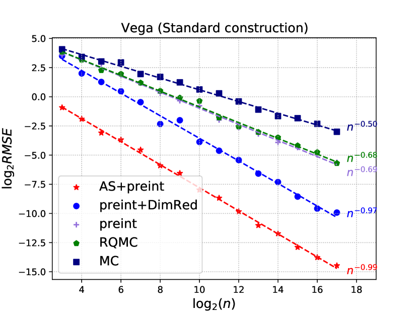
We compare Algorithm 1 with other methods in the option pricing example considered in [44] and [14]. Apart from the payoff function of call option, we also consider the Greeks: Delta, Gamma, Rho, Theta, and Vega. These are defined in [44]. We take the parameters , , , , the same as in [14]. We consider 4 methods:
-
•
AS+pre-int: our proposed active subspace pre-integration method (Algorithm 1), which applies active subspace method to find the direction to pre-integrate,
-
•
pre-int+DimRed: the method proposed in [44], which first pre-integrates and applies GPCA to conduct dimension reduction for the other variables,
-
•
pre-int: pre-integrating with no dimension reduction,
-
•
RQMC: usual RQMC, and
-
•
MC: plain Monte Carlo.
We vary from to . For each , we repeat the simulation 50 times and compute the root mean squared error (RMSE) defined by
where is the estimate in the -th replicate. The true value is approximated by applying pre-int+DimRed using PCA construction with RQMC samples and averaging over 30 independent replicates. We chose this one because it works well and we wanted to avoid using AS-pre-int in case the model used for ground truth had some advantage in reported accuracy.
The root mean square error (RMSE) is plotted versus the sample size on the log-log scale. For the methods AS+pre-int and pre-int+DimRed, we use samples to estimate as in (13). We approximate the gradients of the original integrand and the pre-integrated integrand by the finite difference
matching the choice in [44]. We chose a small value of to keep the costs comparable to plain RQMC. Also because is a local optimum of , we have so there are diminishing returns to accurate estimation of . Finally, any where varies along brings a variance reduction.
We consider both the standard construction (Figure 1) and the PCA construction (Figure 2) of Brownian motion. Several observations are in order:
-
(a)
With the standard construction, AS+pre-int dominates all the other methods for five of the six test functions and is tied for best with pre-int+DimRed for the other one (Gamma).
-
(b)
With the PCA construction, AS+pre-int, pre-int+DimRed and pre-int are the best methods for the payoff, Delta, Theta, and Vega and are nearly equally good.
-
(c)
For Rho, pre-int+DimRed and pre-int are best, while for Gamma, AS+pre-int is best.
The performance of active subspace pre-integration is the same under either the standard or the PCA construction by invariance. For these Asian options it is already well known that the PCA is especially effective. Active subspace pre-integration finds something almost as good without special knowledge, coming out better in one example, worse in another and essentially the same in the other four.


5.2 Basket option
A basket option depends on the weighted average of several assets. Suppose that the assets follow the SDE
where are standard Brownian motions with correlation
for all . For some nonnegative weights , the payoff function of the Asian basket call option is given by
where is the arithmetic average of in the time interval . Here, we only consider assets. To generate with correlation , we can generate two independent standard Brownian motions letting
Following the same discretization as before, we can generate . Then for time steps , let
Again, the matrix can be constructed by the standard construction or the PCA construction. Thus, the expected payoff can be written as
where the expectation is taken over .
In the pre-integration step, we choose to integrate out . This can be easily carried out as in equations (15) and (16) provided that the first column of is nonnegative. We take , , , and . The RMSE values are plotted in Figure 3. In the left panel, we take , , , , and . In the right panel, we take , , , , and . This reverses the roles of the two assets which will make a difference when one pre-integrates over the first of the inputs. We use as before. In the top row of Figure 3, the matrix is obtained by the standard construction, while in the bottom row, is obtained by the PCA construction.


A few observations are in order:
-
(a)
For the standard construction, pre-integrating over brings little improvement over plain RQMC. But for PCA construction, pre-integrating over brings a big variance reduction.
-
(b)
The dimension reduction technique from [44] largely improves the RMSE from pre-integration without dimension reduction. This improvement is particularly significant for the standard construction.
-
(c)
Active subspace pre-integration, AS+preint, has the best performance for both the standard and PCA constructions. It is even better than pre-integrating out the first principal component of Brownian motion with dimension reduction. In this example, the active subspace method is able to find a better direction than the first principal component over which to pre-integrate.
This problem required Brownian motions and the above examples used the same decomposition to sample them both. A sharper principal components analysis would merge the two Brownian motions into a single -dimensional process and use the principal components from their joint covariance matrix. We call this the full PCA construction as described next.
The processes , and , have joint distribution
Let be the joint covariance matrix above. An alternative generation method is to pick with , and let
The matrix can be found by either a Cholesky decomposition or eigendecomposition of . We call this method full standard construction or full PCA construction. Taking , and , it is equivalent to taking
We call this the ordinary PCA or standard construction depending on whether is from the PCA or standard construction.
Figure 4 compares results using this full PCA construction. All methods apply pre-integration before using RQMC. For active subspace pre-integration, we pre-integrate along the direction in 2d found by the active subspace method. For “full PCA”, we pre-integrate along the first principal component of . We can see that active subspace pre-integration has a better RMSE than even the full PCA construction with dimension reduction, which we consider to be the natural generalization of the PCA construction to this setting.


5.3 Timing
Pre-integration changes the computational cost of RQMC and this has not been much studied in the literature. Our figures compare the RMSE of different samplers as a function of the number of evaluations. Efficiency depends also on running times. Here we make study of running times for the pre-integration methods we studied. It is brief in order to conserve space. Running times depend on implementation details that could make our efficiency calculations differ from others’. All of timings we report were conducted on a MacBook Pro with 8 cores and 16GB memory. We simulated them all with replicates and . The standard errors of the average evaluation times were negligible, about %–% of the corresponding means. We also computed times to find and (defined in equations (13) and (14)). Those had small standard errors too, and their costs are a small fraction of the total. The costs of finding the eigendecompositons are negligible in our examples.
Table 1 shows the results of our timings. For the 6 integrands, we find that pre-integration raises the cost of computation by roughly to -fold. That extra cost is not enough to offset the gains from pre-integration with large except for pre-integration of the first component in the standard construction. That variable is not very important and we might well have expected pre-integration to be unhelpful for it.
Most of the pre-integrated computations took about the same amount of time but plain pre-integration and pre-integration with dimension reduction take slighly more time for the standard construction. Upon investigation we found that those methods took slightly more Newton iterations on average. In hindsight this makes sense. The Newton iterations started at . In the standard construction, the first variable does not have a very strong effect on the option value, requiring it to take larger values to reach the positivity threshold and hence (a few) more iterations.
Another component of cost for active subspace methods is in computing an approximation to and . We used function evaluations. Those are about times as expensive as evaluations because they use divided differences. One advantage of active subspace pre-integration is that it uses divided differences of the original integrand. Pre-integration plus dimension reduction requires divided differences of the pre-integrated function with associated Newton searches, and that costs more.
| MC | RQMC | pre-int | AS+pre-int | pre-int+DimRed | |||
|---|---|---|---|---|---|---|---|
| Payoff | 0.6 | 0.6 | 7.5 | 6.9 | 7.4 | 0.3 | 2.9 |
| 0.6 | 0.6 | 6.9 | 6.9 | 6.9 | 0.3 | 2.7 | |
| Delta | 0.5 | 0.4 | 5.7 | 5.2 | 5.7 | 0.2 | 2.2 |
| 0.5 | 0.4 | 5.1 | 5.2 | 5.2 | 0.2 | 2.0 | |
| Gamma | 0.6 | 0.6 | 12.2 | 12.2 | 12.3 | 0.2 | 4.7 |
| 0.6 | 0.6 | 11.7 | 12.3 | 11.7 | 0.2 | 4.5 | |
| Rho | 0.9 | 0.9 | 10.6 | 10.1 | 10.6 | 0.3 | 4.1 |
| 0.9 | 0.9 | 10.1 | 10.2 | 10.1 | 0.4 | 3.9 | |
| Theta | 1.0 | 1.0 | 13.9 | 13.3 | 14.0 | 0.4 | 5.4 |
| 1.0 | 1.0 | 13.4 | 13.4 | 13.4 | 0.4 | 5.2 | |
| Vega | 0.6 | 0.6 | 9.7 | 9.1 | 9.7 | 0.3 | 3.7 |
| 0.6 | 0.6 | 9.1 | 9.1 | 9.1 | 0.3 | 3.5 |
6 Discussion
In this paper we have studied a kind of conditional RQMC known as pre-integration. We found that, just like conditional MC, the procedure can reduce variance but cannot increase it. We proposed to pre-integrate over the first component in an active subspace approximation, which is also known as the gradient PCA approximation. We showed a close relationship between this choice of pre-integration variable and what one would get using a computationally infeasible but well motivated choice by maximizing the Sobol’ index of a linear combination of variables.
In the numerical examples of option pricing, we see that active subspace pre-integration achieves a better RMSE than previous methods when using the standard construction of Brownian motion. For the PCA construction, the proposed method has comparable accuracy in four of six cases, is better once and is worse once. For those six integrands, the PCA construction is already very good. Active subspace pre-integration still provides an automatic way to choose the pre-integration direction. Even using the standard construction it is almost as good as pre-integration with the PCA construction. It can be used in settings where there is no strong incumbent decomposition analogous to the PCA for the Asian option. We saw it perform well for basket options. We even saw an improvement for Gamma in the very well studied case of the Asian option with the PCA construction.
We note that active subspaces use an uncentered PCA analysis of the matrix of sample gradients. One could use instead a centered analysis of where . The potential advantage of this is that is the gradient of which subtracts a linear approximation from before searching for . The rationale for this alternative is that RQMC might already do well integrating a linear function and we would then want to choose a direction that performs well for the nonlinear part of . In our examples, we found very little difference between the two methods and so we proposed the simpler uncentered active subspace pre-integration.
Acknowledgments
This work was supported by the U.S. National Science Foundation under grant IIS-1837931.
References
- [1] P. Acworth, M. Broadie, and P. Glasserman. A comparison of some Monte Carlo techniques for option pricing. In H. Niederreiter, P. Hellekalek, G. Larcher, and P. Zinterhof, editors, Monte Carlo and quasi-Monte Carlo methods ’96, pages 1–18. Springer, 1997.
- [2] L. H. Y. Chen. An inequality for the multivariate normal distribution. Journal of Multivariate Analysis, 12(2):306–315, 1982.
- [3] P. G. Constantine. Active subspaces: Emerging ideas for dimension reduction in parameter studies. SIAM, Philadelphia, 2015.
- [4] P. G. Constantine, E. Dow, and Q. Wang. Active subspace methods in theory and practice: applications to kriging surfaces. SIAM Journal on Scientific Computing, 36(4):A1500–A1524, 2014.
- [5] P. J. Davis and P. Rabinowitz. Methods of Numerical Integration. Academic Press, San Diego, 2nd edition, 1984.
- [6] J. Dick, F. Y. Kuo, and I. H. Sloan. High-dimensional integration: the quasi-Monte Carlo way. Acta Numerica, 22:133–288, 2013.
- [7] J. Dick and F. Pillichshammer. Digital sequences, discrepancy and quasi-Monte Carlo integration. Cambridge University Press, Cambridge, 2010.
- [8] B. Efron and C. Stein. The jackknife estimate of variance. Annals of Statistics, 9(3):586–596, 1981.
- [9] A. D. Gilbert, F. Y. Kuo, and I. H. Sloan. Preintegration is not smoothing when monotonicity fails. Technical report, arXiv:2112.11621, 2021.
- [10] P. Glasserman. Monte Carlo Methods in Financial Engineering, volume 53. Springer, 2004.
- [11] P. Glasserman, P. Heidelberger, and P. Shahabuddin. Asymptotically optimal importance sampling and stratification for pricing path-dependent options. Mathematical finance, 9(2):117–152, 1999.
- [12] A. Griewank, F. Y. Kuo, H. Leövey, and I. H. Sloan. High dimensional integration of kinks and jumps—smoothing by preintegration. Journal of Computational and Applied Mathematics, 344:259–274, 2018.
- [13] J. M. Hammersley. Conditional Monte Carlo. Journal of the ACM (JACM), 3(2):73–76, 1956.
- [14] Z. He. On the error rate of conditional quasi–Monte Carlo for discontinuous functions. SIAM Journal on Numerical Analysis, 57(2):854–874, 2019.
- [15] F. J. Hickernell. Koksma-Hlawka inequality. Wiley StatsRef: Statistics Reference Online, 2014.
- [16] W. Hoeffding. A class of statistics with asymptotically normal distribution. Annals of Mathematical Statistics, 19(3):293–325, 1948.
- [17] C. R. Hoyt and A. B. Owen. Mean dimension of ridge functions. SIAM Journal on Numerical Analysis, 58(2):1195–1216, 2020.
- [18] J. Imai and K. S. Tan. Minimizing effective dimension using linear transformation. In Monte Carlo and Quasi-Monte Carlo Methods 2002, pages 275–292. Springer, 2004.
- [19] M. J. W. Jansen. Analysis of variance designs for model output. Computer Physics Communications, 117(1–2):35–43, 1999.
- [20] I. T. Jolliffe. A note on the use of principal components in regression. Journal of the Royal Statistical Society: Series C (Applied Statistics), 31(3):300–303, 1982.
- [21] P. L’Ecuyer and C. Lemieux. A survey of randomized quasi-Monte Carlo methods. In Modeling Uncertainty: An Examination of Stochastic Theory, Methods, and Applications, pages 419–474. Kluwer Academic Publishers, 2002.
- [22] J. Matoušek. On the L2–discrepancy for anchored boxes. Journal of Complexity, 14(4):527–556, 1998.
- [23] B. Moskowitz and R. E. Caflisch. Smoothness and dimension reduction in quasi-Monte Carlo methods. Mathematical and Computer Modelling, 23(8-9):37–54, 1996.
- [24] H. Niederreiter. Random Number Generation and Quasi-Monte Carlo Methods. SIAM, Philadelphia, PA, 1992.
- [25] G. Ökten and A. Göncü. Generating low-discrepancy sequences from the normal distribution: Box–Muller or inverse transform? Mathematical and Computer Modelling, 53(5-6):1268–1281, 2011.
- [26] A. B. Owen. Randomly permuted -nets and -sequences. In Monte Carlo and Quasi-Monte Carlo Methods in Scientific Computing, pages 299–317, New York, 1995. Springer-Verlag.
- [27] A. B. Owen. Monte Carlo variance of scrambled net quadrature. SIAM Journal of Numerical Analysis, 34(5):1884–1910, 1997.
- [28] A. B. Owen. Scrambled net variance for integrals of smooth functions. Annals of Statistics, 25(4):1541–1562, 1997.
- [29] A. B. Owen. Scrambling Sobol’ and Niederreiter-Xing points. Journal of Complexity, 14(4):466–489, December 1998.
- [30] A. B. Owen. Local antithetic sampling with scrambled nets. Annals of Statistics, 36(5):2319–2343, 2008.
- [31] A. B. Owen. Monte Carlo Theory, Methods and Examples. statweb.stanford.edu/~owen/mc, 2013.
- [32] A. B. Owen and D. Rudolf. A strong law of large numbers for scrambled net integration. SIAM Review, 63(2):360–372, 2021.
- [33] Z. Pan and A. B. Owen. The nonzero gain coefficients of Sobol’s sequences are always powers of two. Technical Report arXiv:2106.10534, Stanford University, 2021.
- [34] A. Papageorgiou. The Brownian bridge does not offer a consistent advantage in quasi-Monte Carlo integration. Journal of Complexity, 18(1):171–186, 2002.
- [35] M. T. Parente, J. Wallin, and B. Wohlmuth. Generalized bounds for active subspaces. Electronic Journal of Statistics, 14(1):917–943, 2020.
- [36] G. Pirsic. Schnell konvergierende Walshreihen über gruppen. Master’s thesis, University of Salzburg, 1995. Institute for Mathematics.
- [37] S. Razavi, A. Jakeman, A. Saltelli, C. Prieur, B. Iooss, E. Borgonovo, E. Plischke, S. L. Piano, T. Iwanaga, W. Becker, S. Tarantola, J. H. A. Guillaume, J. Jakeman, H. Gupta, N. Melillo, G. Rabitti, V. Chabirdon, Q. Duan, X. Sun, S. Smith, R. Sheikholeslami, N. Hosseini, M. Asadzade, A. Puy, S. Kucherenko, and H. R. Maier. The future of sensitivity analysis: an essential discipline for systems modeling and policy support. Environmental Modelling & Software, 137:104954, 2021.
- [38] C. P. Robert and G. O. Roberts. Rao-Blackwellization in the MCMC era. Technical Report arXiv:2101.01011, University of Warwick, 2021.
- [39] I. M. Sobol’. The distribution of points in a cube and the accurate evaluation of integrals. USSR Computational Mathematics and Mathematical Physics, 7(4):86–112, 1967.
- [40] I. M. Sobol’. Multidimensional Quadrature Formulas and Haar Functions. Nauka, Moscow, 1969. (In Russian).
- [41] I. M. Sobol’. Sensitivity estimates for nonlinear mathematical models. Mathematical Modeling and Computational Experiment, 1:407–414, 1993.
- [42] I. M. Sobol’ and S. Kucherenko. Derivative based global sensitivity measures and their link with global sensitivity indices. Mathematics and Computers in Simulation (MATCOM), 79(10):3009–3017, 2009.
- [43] H. F. Trotter and J. W. Tukey. Conditional Monte Carlo for normal samples. In Symposium on Monte Carlo Methods, pages 64–79, New York, 1956. Wiley.
- [44] Y. Xiao and X. Wang. Conditional quasi-Monte Carlo methods and dimension reduction for option pricing and hedging with discontinuous functions. Journal of Computational and Applied Mathematics, 343:289–308, 2018.
- [45] Y. Xiao and X. Wang. Enhancing quasi-Monte Carlo simulation by minimizing effective dimension for derivative pricing. Computational Economics, 54(1):343–366, 2019.
- [46] R.-X. Yue and S.-S. Mao. On the variance of quadrature over scrambled nets and sequences. Statistics & Probability Letters, 44(3):267–280, 1999.
- [47] C. Zhang, X. Wang, and Z. He. Efficient importance sampling in quasi-Monte Carlo methods for computational finance. SIAM Journal on Scientific Computing, 43(1):B1–B29, 2021.