PR-GCN: A Deep Graph Convolutional Network with Point Refinement
for 6D Pose Estimation
Abstract
RGB-D based 6D pose estimation has recently achieved remarkable progress, but still suffers from two major limitations: (1) ineffective representation of depth data and (2) insufficient integration of different modalities. This paper proposes a novel deep learning approach, namely Graph Convolutional Network with Point Refinement (PR-GCN), to simultaneously address the issues above in a unified way. It first introduces the Point Refinement Network (PRN) to polish 3D point clouds, recovering missing parts with noise removed. Subsequently, the Multi-Modal Fusion Graph Convolutional Network (MMF-GCN) is presented to strengthen RGB-D combination, which captures geometry-aware inter-modality correlation through local information propagation in the graph convolutional network. Extensive experiments are conducted on three widely used benchmarks, and state-of-the-art performance is reached. Besides, it is also shown that the proposed PRN and MMF-GCN modules are well generalized to other frameworks.
1 Introduction
6D pose estimation aims to predict the orientation and location of an object in the 3D space from a canonical frame. It has received extensive attention in computer vision, since it is one of the fundamental steps for a wide range of applications, such as robotics grasping [6, 35, 47] and augmented reality [22, 23]. Traditional methods [10, 11] attempt to accomplish this task based on RGB images only. They adopt handcraft features (e.g. SIFT [21] and SURF [1]) to establish correspondence between input and canonical images. Inspired by the great success in detection/recognition, deep neural networks are recently explored to address this issue, including the single-stage regression methods [15] and key-point based methods [13, 32, 36, 35, 26, 25, 20]. Despite the remarkable promotion in accuracy, RGB-based deep models heavily rely on textures; thus sensitive to illumination variations, severe occlusions, and cluttered backgrounds.
Along with the emergence and innovation of depth sensors, 6D pose estimation on RGB-D data has become popular, expecting to deliver performance gain by adding geometry information. Early works [11, 24, 45] estimate object poses from RGB images and refine them according to depth maps. Later studies [38, 17] dedicate to integrating RGB and depth clues in a more sophisticated way. Particularly, [41, 31, 30, 38, 9] represent depth images as 3D point clouds and the models are more efficient in computation and storage than those on original depth maps. By jointly making use of both modalities, RGB-D based solutions report better scores, with the superiority in the presence of the difficulties aforementioned as well as the low-texture case.
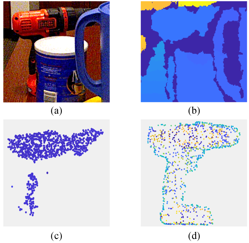
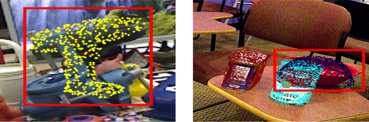
However, current RGB-D pose estimation suffers from two major limitations: ineffective representation of depth data and insufficient combination of two modalities. For the former, as captured in cluttered scenes, depth information is usually noisy and incomplete (see Fig. 1). Inferring poses from such data, either in 2D depth maps or 3D point clouds, is not robust, leading to accuracy deterioration. For the latter, RGB and depth clues are fused by concatenating separately learned single-modal features [38] or by applying a simple point-wise encoder [9], where inter-modality correlations are not considered or roughly modeled in a global manner, leaving much room for improvement.
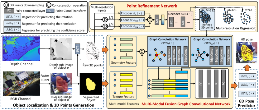
In this paper, we propose a novel deep learning approach, namely Graph Convolutional Network with Point Refinement (PR-GCN), to simultaneously address the two limitations in a unified way. As in Fig. 2, given the RGB image and 3D point cloud (generated from depth map) of an object, we first introduce a Point Refinement Network (PRN) to polish the point cloud. Endowed with an encoder-decoder structure and trained with a regularized multi-resolution regression loss, PRN recovers the missing parts of the raw input with noise removed. Subsequently, we integrate RGB-D clues by a Mutli-Modal Fusion Graph Convolutional Network (MMF-GCN). It constructs a -Nearest Neighbor (-NN) graph and extracts geometry-aware inter-modality correlation through local information propagation in the Graph Convolutional Network (GCN). An additional -NN graph and GCN are employed to encode local geometry attributes of the refined point cloud as a complement to the original data. The features from the two GCNs are then combined and fed into several fully-connected layers for final 6D pose prediction. We extensively evaluate PR-GCN on three public benchmarks, Linemod [11], Occlusion Linemod [2], and YCB-Video [40], and achieve the state-of-the-art performance. We also show that the proposed PRN and MMF-GCN modules are well generalized to other frameworks.
The contributions: 1) We propose the PR-GCN approach to 6D pose estimation by enhancing depth representation and multi-modal combination. 2) We present the PRN module with a regularized multi-resolution regression loss for point-cloud refinement. To the best of our knowledge, it is the first that applies 3D point generation to this task. 3) We develop the MMF-GCN module to capture local geometry-aware inter-modality correlation for RGB-D fusion.
2 Related Work
RGB based 6D Pose Estimation. The traditional methods [11, 7, 16] establish correspondence between object appearances and poses from single RGB images. Linemod [11] predicts poses by modeling the relationship between texture gradients and surface normals on 3D templates. [3] exploits key-points of specific objects for pose estimation by iteratively matching them between input and canonical frames. As in other vision tasks, deep models are also investigated to build more powerful features for this issue. DeepIM [18] adopts CNNs to learn reliable representations for template-matching. BB8 [32] applies CNNs in a multi-stage segmentation scheme to regress key-point coordinates. PVNet [29] proposes a deep offset prediction model to alleviate negative impacts of occlusions. CDPN [19] and Pix2pose [28] map 3D coordinates to 2D pixels and regress pose parameters on 2D images. LatentFusion [27] handles unseen object poses by reconstructing a latent 3D representation.
RGB-D based 6D Pose Estimation. With geometry information, depth maps contribute to pose estimation for various lighting conditions and low-textured appearances, complementary to RGB images. MCN [17] employs two CNNs for representation learning in RGB and depth respectively and resulting features are then concatenated for pose prediction. PoseCNN [40] and SSD-6D [14] follow the coarse-to-fine scheme, where poses are initially estimated on RGB frames and subsequently refined on depth maps. [37] builds a multi-view model to jointly reconstruct whole scenes and optimize multi-object poses.
Recently, there has emerged a trend to represent geometry clues in 3D point clouds rather than depth mas for higher efficiency [38, 5, 4, 31, 9]. DenseFusion [38] designs a heterogeneous network to integrate texture and shape features and such representation proves more discriminative than single-modal ones. CF [5] introduces attention modules to combine the two modalities for further improvements. G2L [4] segments point clouds of objects in scenes by frustum pointnet [31] and regresses pose parameters via extra coordinate constraints. PVN3D [9] incorporates DenseFusion into 3D key-point detection and instance semantic segmentation, significantly boosting the performance.
Unfortunately, the point clouds generated from the depth maps are often of a low quality, since the shape information is often incomplete and noisy as Fig. 1 shows. Besides, the combination of RGB and depth clues is launched in a very rough way, e.g., directly concatenating or point-wise encoding. In contrast, our approach develops the PRN and MMF-GCN modules to polish depth clues by generating refined point clouds and enhance integration by capturing local geometry-aware inter-modality correlations respectively, both of which are beneficial to pose estimation.
3 The Proposed Method
3.1 Framework Overview
RGB-D based 6D pose estimation recovers 6D poses of objects in RGB-D images, where 6D pose is usually represented by a rotation matrix and a translation vector . For this issue, we propose the PR-GCN approach. As Fig. 2 depicts, it consists of four steps: object localization and 3D points generation, 3D points refinement, GCN-based multi-modal fusion, and 6D pose prediction.
Object Localization and 3D Points Generation. Given an RGB-D image , we firstly locate objects on using the off-the-shelf Faster R-CNN [33] detector, where and denote the RGB and depth channels of . According to the detected bounding boxes, we crop the sub-images , each of which contains an instance . and are the RGB and depth channels of . As in PoseCNN [40], we add a segmentation head to remove background of . With (foreground mask) and , raw 3D points are rendered by Point-Cloud Transform (PCT) [8], where is the number of points and is the 3D coordinate of the -th point. It is worth noting that could be severely incomplete and noisy due to external occlusions and sensor noise (see Fig. 1).
3D Points Refinement. To polish the quality of the generated raw 3D points , we propose the PRN module. As in Fig. 2, it is composed of an MLP-based encoder and a multi-resolution decoder to recover the complete and accurate 3D point cloud , where is the number of refined points. A regularized multi-resolution regression loss is formulated in training, enhancing its ability of filtering out noise in .
GCN-based Multi-Modal Fusion. For more sufficient RGB-D fusion, we propose the MMF-GCN module. As in Fig. 2, it extracts texture and geometry features from and , respectively, and a graph is built based on geometry distribution. Accordingly, and are initially integrated by applying a GCN on the previously built graph through local information propagation. The geometry clues from the refined 3D points are encoded by introducing an extra GCN and then incorporated into the initially fused features, which are fed into several stacked fully-connected layers for further fusion. The resulting feature is therefore the multi-modal representation for successive 6D pose estimation, where and refer to the number of points and the feature dimension, respectively. Since MMF-GCN captures local geometry-aware inter-modality correlation and leverages refined 3D point clouds, it is expected to deliver more discriminative and robust features.
6D Pose Prediction. is finally fed into three regression branches: , , , for rotations , translations , confidence scores , respectively. Each branch has four fully-connected layers. Similar to [9, 29, 38], we select the candidate with the highest confidence score as the estimated pose, formulated as:
| (1) |
3.2 Point Refinement Network
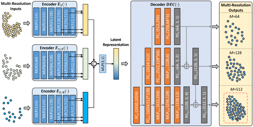
Recall that PRN aims to generate the refined 3D point cloud from the raw one of a low quality . As in Fig. 3, PRN is endowed with an encoder-decoder architecture. To deal with the change in point density (resolution), we downsample with and scales, resulting in two extra point clouds: and .
Accordingly, the encoder has three branches , , , whose inputs are , , and outputs are the three representations , , . Each branch is a stack of six MLP layers. The concatenation of , and followed by an MLP layer forms the intermediate latent representation .
The decoder employs a multi-resolution structure as [43] does. The first branch with four fully-connected (FC) layers as well as one reshape (RS) operation is built to obtain the coarse point cloud of a low-resolution (or equivalently). The second branch consists of the first two shared FC layers, one additional FC layer, one MLP layer and one RS operation, generating a mediate-resolution point cloud Then, is integrated into by a broadcasting additive operation , and is reshaped into . Similarly, the third branch finally renders a high-resolution point cloud by sharing the first FC layer, adding one FC layer, three MLP layers and one RS operation, and incorporating the mediate-resolution information as
For training PRN, we develop a multi-resolution regression loss formulated as follows:
| (2) |
where is ground-truth point cloud of object . is the Chamfer distance defined as , given and .
In Eq. (2), is forced to fit the ground-truth in low-to-high resolutions when minimizing . In other words, is forced to predict high-quality points in multiple resolutions by a unified structure, and thus optimized with more supervision than the single-resolution case. Moreover, as shown in Fig. 3, the high-resolution output integrates multi-resolution information from and . As a consequence, PRN mitigates the incompleteness and decreases the noise of the raw 3D points.
Despite the aforementioned advantages of , it fails to perceive the global point distribution of . We handle this problem by introducing the adversarial loss:
| (3) |
where is the discriminator to classify whether a point belongs to (“real”) or not (“fake”). By minimizing , PRN is expected to generate that captures holistic point distribution of , benefiting the quality of .
The regularized multi-resolution regression loss is thus formulated as:
| (4) |
where and are the trade-off hyper-parameters.
3.3 Multi-Modal Fusion GCN
| RGB based methods | RGB-D based methods | |||||||||||
|---|---|---|---|---|---|---|---|---|---|---|---|---|
| Object | PoseCNN* | PVNet | CDPN | DPOD | DPVL | PF* | SSD6D† | DF* | PVN3D | G2L* | Ours* | Ours |
| [40, 18] | [29] | [19] | [44] | [42] | [41] | [14] | [38] | [9] | [4] | |||
| ape | 77.0 | 43.6 | 64.4 | 87.7 | 69.1 | 70.4 | 65.0 | 92.3 | 97.3 | 96.8 | 97.6 | 99.2 |
| benchvise | 97.5 | 99.9 | 97.8 | 98.5 | 100.0 | 80.7 | 80.0 | 93.2 | 99.7 | 96.1 | 99.2 | 99.8 |
| camera | 93.5 | 86.9 | 91.7 | 96.1 | 94.1 | 60.8 | 78.0 | 94.4 | 99.6 | 98.2 | 99.4 | 100.0 |
| can | 96.5 | 95.5 | 95.9 | 99.7 | 98.5 | 61.1 | 86.0 | 93.1 | 99.5 | 98.0 | 98.4 | 99.4 |
| cat | 82.1 | 79.3 | 83.8 | 94.7 | 83.1 | 79.1 | 70.0 | 96.5 | 99.8 | 99.2 | 98.7 | 99.8 |
| driller | 95.0 | 96.4 | 96.2 | 98.8 | 99.0 | 47.3 | 73.0 | 87.0 | 99.3 | 99.8 | 98.8 | 99.8 |
| duck | 77.7 | 52.6 | 66.8 | 86.3 | 63.5 | 63.0 | 66.0 | 92.3 | 98.2 | 97.7 | 98.9 | 98.7 |
| eggbox | 97.1 | 99.2 | 99.7 | 99.9 | 100.0 | 99.9 | 100.0 | 99.8 | 99.8 | 100.0 | 99.9 | 99.6 |
| glue | 99.4 | 95.7 | 99.6 | 96.8 | 98.0 | 99.3 | 100.0 | 100.0 | 100.0 | 100.0 | 100.0 | 100.0 |
| holepuncher | 52.8 | 82.0 | 85.8 | 86.9 | 88.2 | 71.8 | 49.0 | 92.1 | 99.9 | 99.0 | 99.4 | 99.8 |
| iron | 98.3 | 98.9 | 97.9 | 100.0 | 99.9 | 83.2 | 78.0 | 97.0 | 99.7 | 99.3 | 98.5 | 99.5 |
| lamp | 97.5 | 99.3 | 97.9 | 96.8 | 99.8 | 62.3 | 73.0 | 95.3 | 99.8 | 99.5 | 99.2 | 100.0 |
| phone | 87.7 | 92.4 | 90.8 | 94.7 | 96.4 | 78.8 | 79.0 | 92.8 | 99.5 | 98.9 | 98.4 | 99.7 |
| MEAN | 88.6 | 86.3 | 89.9 | 95.2 | 91.5 | 73.7 | 79.0 | 94.3 | 99.4 | 98.7 | 98.9 | 99.6 |
As mentioned before, given the RGB () and point cloud ( and ) data of object , MMF-GCN integrates multi-modal information into more effective representation () for accurate 6D pose estimation.
Specifically, MMF-GCN first extracts the geometry feature from and the texture feature from for the -th point . The normalized coordinate of is directly used as the geometry feature, and by mapping this coordinate to the pixel on , PSPNet [46] with the ResNet-18 backbone is adopted to compute pixel-wise representation as the texture feature.
When and are ready, a -Nearest Neighbor (NN) graph is constructed. and denote the vertices and the edges, and indicates the nearest neighbors of . The edge feature is defined as with , where is a nonlinear function parameterized by .
Afterwards, a graph convolution network is employed to capture local inter-modality correlations, with EdgeConv [39] for graph convolutions. The basic updating scheme is formulated as:
where denotes the -th edge feature in the -th layer, is a nonlinear function in the -th layer, and refers to max pooling. The representation is then obtained, where ; and are the point number and the feature dimension, respectively.
As is usually incomplete and noisy, MMF-GCN encodes the geometry attribute of and incorporates it into as a complement. Concretely, similar to , another -NN graph is built based on , and an extra GCN is employed. The refined geometry feature is calculated using EdgeConv: , where and is the feature dimension. is subsequently combined with through simple concatenation, which is further integrated by a few stacked FC layers . At last, multi-modal representation is formed as for 6D pose estimation.
3.4 Training Objectives
The objective function for training PR-GCN consists of two parts: the pose estimation loss and the regularized multi-resolution regression loss as depicted in Eq. (4).
Given the ground-truth 6D pose and the predictions at points , the pose estimation error of the -th prediction is defined as . Based on , we adopt an extra regularization term on the prediction scores as in [38] and formulate the pose estimation loss as:
| (5) |
| (6) |
where is the trade-off hyper-parameter.
4 Experiments
4.1 Datasets and Metrics
Extensive evaluation is made on three datasets: Linemod [11], Occlusion Linemod [2] and YCB-Video [40].
Linemod [11] is composed of 15 RGB-D videos of 15 low-textured objects. Following [32], 13 objects are considered and the standard training/testing split is adopted as in [38, 40]. Occlusion Linemod is collected by annotating a subset of Linemod (8 out of 15 objects), where each image has multiple occluded objects, making it more challenging. YCB-Video [40] includes 21 objects with various textures and sizes. It provides RGB-D images and detailed pose annotations. There are 130K real images from 92 videos and 80K synthetically rendered ones, and 16,189 real and all the synthesized images are used in training, according to [38].
| Object | PoseCNN [40] | DeepHeat [26] | SS [12] | Pix2pose [28] | PVNet [29] | HybridPose [34] | PVN3D [9] | Ours |
|---|---|---|---|---|---|---|---|---|
| Ape | 9.6 | 12.1 | 17.6 | 22.0 | 15.8 | 20.9 | 33.9 | 40.2 |
| Can | 45.2 | 39.9 | 53.9 | 44.7 | 63.3 | 75.3 | 88.6 | 76.2 |
| Cat | 0.9 | 8.2 | 3.3 | 22.7 | 16.7 | 24.9 | 39.1 | 57.0 |
| Driller | 41.4 | 45.2 | 62.4 | 44.7 | 65.7 | 70.2 | 78.4 | 82.3 |
| Duck | 19.6 | 17.2 | 19.2 | 15.0 | 25.2 | 27.9 | 41.9 | 30.0 |
| Eggbox | 22.0 | 22.1 | 25.9 | 25.2 | 50.2 | 52.4 | 80.9 | 68.2 |
| Glue | 38.5 | 35.8 | 39.6 | 32.4 | 49.6 | 53.8 | 68.1 | 67.0 |
| Holepuncher | 22.1 | 36.0 | 21.3 | 49.5 | 39.7 | 54.2 | 74.7 | 97.2 |
| MEAN | 24.9 | 27.0 | 27.0 | 32.0 | 40.8 | 47.5 | 63.2 | 65.0 |
| PoseCNN+ICP [40] | DenseFusion [38] | PVN3D [9] | CF [5] | G2L [4] | Ours | ||||||
|---|---|---|---|---|---|---|---|---|---|---|---|
| AUC | <2cm | AUC | <2cm | AUC | <2cm | AUC | <2cm | AUC | AUC | <2cm | |
| 002_master_chef_can | 95.8 | 100.0 | 96.4 | 100.0 | 96.0 | 100.0 | 92.5 | 98.7 | 94.0 | 97.1 | 100.0 |
| 003_cracker_box | 92.7 | 91.6 | 95.5 | 99.5 | 96.1 | 100.0 | 95.4 | 98.6 | 88.7 | 97.6 | 100.0 |
| 004_sugar_box | 98.2 | 100.0 | 97.5 | 100.0 | 97.4 | 100.0 | 96.7 | 99.9 | 96.0 | 98.3 | 100.0 |
| 005_tomato_soup_can | 94.5 | 96.9 | 94.6 | 96.9 | 96.2 | 98.1 | 92.0 | 95.8 | 86.4 | 95.3 | 97.6 |
| 006_mustard_bottle | 98.6 | 100.0 | 97.2 | 100.0 | 97.5 | 100.0 | 94.8 | 97.5 | 95.9 | 97.9 | 100.0 |
| 007_tuna_fish_can | 97.1 | 100.0 | 96.6 | 100.0 | 96.0 | 100.0 | 88.8 | 84.1 | 84.1 | 97.6 | 100.0 |
| 008_pudding_box | 97.9 | 100.0 | 96.5 | 100.0 | 97.1 | 100.0 | 93.2 | 98.6 | 93.5 | 98.4 | 100.0 |
| 009_gelatin_box | 98.8 | 100.0 | 98.1 | 100.0 | 97.7 | 100.0 | 95.7 | 100.0 | 96.8 | 96.2 | 94.4 |
| 010_potted_meat_can | 92.7 | 93.6 | 91.3 | 93.1 | 93.3 | 94.6 | 86.2 | 83.9 | 86.2 | 96.6 | 99.1 |
| 011_banana | 97.1 | 99.7 | 96.6 | 100.0 | 96.6 | 100.0 | 92.6 | 98.9 | 96.3 | 98.5 | 100.0 |
| 019_pitcher_base | 97.8 | 100.0 | 97.1 | 100.0 | 97.4 | 100.0 | 95.4 | 98.4 | 91.8 | 98.1 | 100.0 |
| 021_bleach_cleanser | 96.9 | 99.4 | 95.8 | 100.0 | 96.0 | 100.0 | 89.0 | 86.2 | 92.0 | 97.9 | 100.0 |
| 024_bowl | 81.0 | 54.9 | 88.2 | 98.8 | 90.2 | 80.5 | 86.1 | 94.3 | 86.7 | 90.3 | 96.6 |
| 025_mug | 95.0 | 99.8 | 97.1 | 100.0 | 97.6 | 100.0 | 93.5 | 94.8 | 95.4 | 98.1 | 100.0 |
| 035_power_drill | 98.2 | 99.6 | 96.0 | 98.7 | 96.7 | 100.0 | 82.9 | 84.8 | 95.2 | 98.1 | 100.0 |
| 036_wood_block | 87.6 | 80.2 | 89.7 | 94.6 | 90.4 | 93.8 | 92.3 | 99.6 | 86.2 | 96.0 | 100.0 |
| 037_scissors | 91.7 | 95.6 | 95.2 | 100.0 | 96.7 | 100.0 | 90.1 | 89.5 | 83.8 | 96.7 | 100.0 |
| 040_large_marker | 97.2 | 99.7 | 97.5 | 100.0 | 96.7 | 99.8 | 93.9 | 99.8 | 96.8 | 97.9 | 100.0 |
| 051_large_clamp | 75.2 | 74.9 | 72.9 | 79.2 | 93.6 | 93.6 | 70.3 | 76.7 | 94.4 | 87.5 | 93.3 |
| 052_extra_large_clamp | 64.4 | 48.8 | 69.8 | 76.3 | 88.4 | 83.6 | 69.5 | 74.5 | 92.3 | 79.7 | 84.6 |
| 061_foam_brick | 97.2 | 100.0 | 92.5 | 100.0 | 96.8 | 100.0 | 94.6 | 100.0 | 94.7 | 97.8 | 100.0 |
| MEAN | 93.0 | 93.2 | 93.1 | 96.8 | 95.5 | 97.6 | 89.8 | 93.1 | 92.4 | 95.8 | 98.5 |
As in the literature, two main metrics are employed for evaluation, i.e., Average Distance (ADD) [40] and ADD-Symmetric (ADD-S) [40], designed for general objects and symmetric objects, respectively. DenseFusion [38] gives the ADD-S smaller than 2 centimeters (ADD-S2cm) for real applications e.g. robotic manipulation, and PoseCNN [40] and DenseFusion [38] report the Area Under the ADD-S Curve (AUC) with the maximum threshold at 0.1m. We also show them for comparison.
4.2 Implementation Details
We fix the size of RGB images as 480640. The numbers of raw/refined 3D points, i.e., /, are set to 100/512 and 100/1,024 on Linemod (Occlusion Linemod) and YCB-Video, respectively. In MMF-GCN, refined point clouds are down-sampled to 100 points by FPS. When building the graphs and , we utilize 30 nearest neighbors, i.e., . In PRN, the hyper-parameters , and in the overall training loss are set to 0.05, 0.95 and 1.0. To train PR-GCN in a more stable way, PRN and MMF-GCN are progressively optimized. For instance, on YCB-Video, PRN and MMF-GCN are first alternatively trained for 15 epochs and then jointly optimized for 30 epochs.
In PRN training, we adopt the ADAM optimizer with the learning rate of 0.0001 and the batch size of 48. The rest parts of PR-GCN are trained for 40, 20 and 60 epochs on Linemod, Occlusion Linemod and YCB-Video, respectively, where the learning rate is initially set to 0.0001 and decayed by a factor of 0.3 after half of the maximal epochs.
4.3 Comparison with the State-of-the-art Methods
Results on Linemod. We first compare PR-GCN to the state-of-the-art methods on Linemod, including the RGB based models: PoseCNN (+DeepIM) [40, 18], PVNet [29], CDPN [19], DPOD [44] and DPVL [42] and the RGB-D based ones: Point Fusion [41], SSD6D (+ICP) [14], Dense Fusion [38], PVN3D [9] and G2L[4]. Several approaches, denoted by ‘’ or ‘’ in Table 1, only adopt real or synthetic training data, whist the others use both. In our work, we mainly consider the setting with the two types of training data, and also report the performance with real data only.
Table 1 summarizes the ADD(-S) of different methods on Linemod, and we can see that the RGB-D based deep models (e.g., PVN3D and G2L) remarkably outperform the RGB based ones by a large margin due to additional geometry information given by the depth channel. Regarding the RGB-D counterparts, the proposed PR-GCN achieves better performance, which improves PointFusion and DenseFusion by 25.2% and 4.6%, respectively. Our approach also boosts the performance of keypoint-based methods, including PVN3D and G2L. It is worth noting that the second best method, i.e. PVN3D, uses 70,000 synthetic training data, and needs to train different models for distinct object categories. In contrast, our method trains a universal model for all object categories, and merely utilizes 3,500 synthetic training data, which is much more efficient than PVN3D.
Results on Occlusion Linemod. To evaluate the robustness of PR-GCN to inter-object occlusions, we display detailed results on Occlusion Linemod, in comparison with PoseCNN [40], DeepHeat [26], SS [12], Pix2Pose [28], PVNet [29], HybridPose [34] and PVN3D [9]. As shown in Table 2, our method consistently reaches the top ADD(-S) AUC and achieves the best mean ADD(-S) AUC, highlighting its superiority in the presence of heavy occlusions.
Results on YCB-Video. We then extend our analysis on this database and compare PR-GCN with PoseCNN (+ICP) [40], DenseFusion [38], PVN3D [9], CF [5] and G2L [4]. Table 3 shows the AUC and ADD-S<2cm for various methods. It can be observed that our method achieves the highest performance on both the metrics. For instance, compared to PVN3D and DenseFusion, PR-GCN improves the ADD-S2cm by 0.9% and 1.7%, respectively.
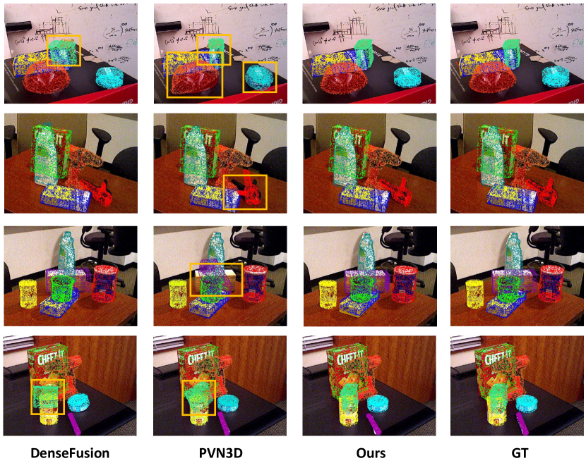
Qualitative results. We additionally provide qualitative results in Fig. 4, comparing to DenseFusion and PVN3D. Due to cluttered backgrounds and severe occlusions, DenseFusion and PVN3D predict inaccurate poses in many cases, while our PR-GCN performs more robustly with much better results. We also demonstrate failure cases in Fig. 4, revealing that PR-GCN fails when dealing with extremely occluded objects and some symmetric ones.
Inference efficiency. Besides the accuracy, we evaluate the efficiency of our method on Linemod. As shown in Table 4, each key component infers fast, and the full pipeline takes 68ms on an Nvidia 1080Ti GPU, which is acceptable in downstream tasks such as robotic grasping.
| Component | Seg | PR | PE | Full |
|---|---|---|---|---|
| Time (s) | 0.030 | 0.008 | 0.030 | 0.068 |
| Method | PRN | MMF-GCN | MEAN |
|---|---|---|---|
| Baseline (with DGCNN) | 94.8 | ||
| Baseline+PRN | 96.8 | ||
| Baseline+MMF-GCN | 96.9 | ||
| Full model | 98.9 |
| Method | PVN3D | DenseFusion | ||
|---|---|---|---|---|
| Metric | ADD-S | <2cm | ADD-S | <2cm |
| Original model | 95.5 | 97.6 | 93.1 | 96.8 |
| w/ PRN | - | - | 94.1 | 97.2 |
| w/ MMF-GCN | 96.2 | 98.4 | 93.5 | 97.2 |
| w/ both | - | - | 94.9 | 98.1 |
| PoseCNN segmentation | PVN3D segmentation | GT segmentation | |||||||
| PoseCNN | DenseFusion | Ours | DenseFusion | PVN3D | Ours | Densefusion | PVN3D | Ours | |
| AUC | 93.0 | 93.1 | 95.0 | 91.8 | 95.5 | 95.8 | 94.5 | 96.4 | 96.9 |
| <2cm | 93.2 | 96.8 | 97.6 | 92.8 | 97.6 | 98.5 | 98.1 | - | 99.9 |
| WO-PRN | PRN-SR | PRN-MR | |
|---|---|---|---|
| ADD-S | 94.0 | 94.6 | 95.8 |
| < 2cm | 97.1 | 96.6 | 98.5 |
4.4 Ablation Study
We comprehensively validate individual components of PR-GCN in the following.
The impact of PRN and MMF-GCN. The baseline method removes PRN and replaces MMF-GCN by DGCNN [39] which adopts the same basic point cloud aggregator as our PR-GCN. As Table 5 displays, PRN boosts the baseline by 2.0%, indicating that refined point clouds contribute to pose estimation, while MMF-GCN achieves an improvement of 2.1%, demonstrating its advantage in integrating multi-modal features. The combination of PRN and MMF-GCN further enhances the performance.
The generalizability of PRN and MMF-GCN. We generalize the PRN and MMF-GCN modules to two state-of-the-art frameworks including PVN3D [9] and DenseFusion [38], and evaluate their performance on YCB-Video. Note that PVN3D cannot utilize PRN directly, since segmentation is required on the whole scene while PRN focuses on specific objects. We thus only evaluate the effect of MMF-GCN on PVN3D. As shown in Table 6, PRN promotes the ADD-S of DenseFusion by 1%, and a similar improvement can be observed when applying MMF-GCN. The results indicate that PRN and MMF-GCN benefit other frameworks for 6D pose estimation.
The influence of segmentation. As in Fig. 2, our framework introduces RGB-based segmentation to extract foreground objects, while PoseCNN [40], DenseFusion [38] and PVN3D [9] adopt different instance segmentation models. To validate the effect of segmentation, we replace the segmentation model in our framework by the counterparts used in PoseCNN and PVN3D as well as the ground-truth, and report their AUC and ADD-S2cm metrics on YCB-Video. Similarly, we evaluate this factor on other frameworks, including PoseCNN, DenseFusion and PVN3D. As reported in Table 7, all these frameworks achieve the highest AUC and ADD-S2cm using ground-truth, indicating that better segmentation boosts the estimation accuracy. Meanwhile, with segmentation alternatives, our framework consistently outperforms the others, showing that PR-GCN is superior, regardless of which segmentation model is used.
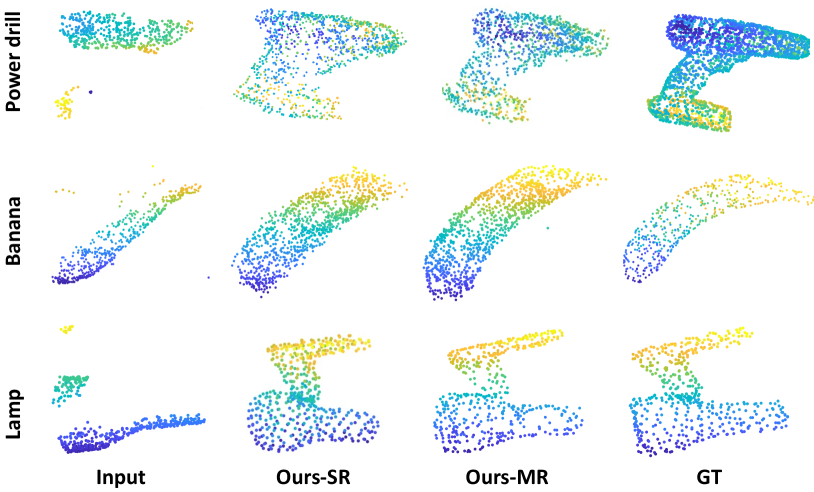
The effect of the multi-resolution regression loss on PRN. We finally validate the credit of the regularized multi-resolution regression loss . For comparison, we apply on only, denoted by PRN-SR, while the multi-resolution case is denoted by PRN-MR. We also report the result without using PRN (WO-PRN). As summarized in Table 8, adopting the single-resolution loss promotes the performance of our method. When the multi-resolution loss is added, ADD-S is further boosted to 95.8%, demonstrating its effectiveness. Moreover, we visualize the generated refined 3D points in Fig. 5, and the results clearly show the advantage of PRN in dealing with the incompleteness and noise, after adding the loss .
5 Conclusion
In this paper, we propose a novel approach, namely deep Graph Convolutional Networks with Point Refinement (PR-GCN), to RGB-D based 6D pose estimation. We develop a Point Refinement Network (PRN) to improve the quality of depth representation, together with a Multi-Modal Fusion Graph Convolution Network (MMF-GCN) to fully explore local geometry-aware inter-modality correlations for sufficient combination. Extensive experiments validate its superiority and the PRN and MMF-GCN modules.
Acknowledgment
This work is partly supported by the National Natural Science Foundation of China (No. 62022011), the Research Program of State Key Laboratory of Software Development Environment (SKLSDE-2021ZX-04), and the Fundamental Research Funds for the Central Universities.
References
- [1] Herbert Bay, Andreas Ess, Tinne Tuytelaars, and Luc Van Gool. Speeded-up robust features (SURF). Computer Vision and Image Understanding, 110(3):346–359, 2008.
- [2] Eric Brachmann, Alexander Krull, Frank Michel, Stefan Gumhold, Jamie Shotton, and Carsten Rother. Learning 6d object pose estimation using 3d object coordinates. In European Conference on Computer Vision, pages 536–551, 2014.
- [3] Eric Brachmann, Alexander Krull, Frank Michel, Stefan Gumhold, Jamie Shotton, and Carsten Rother. Learning 6d object pose estimation using 3d object coordinates. In European Conference on Computer Vision, pages 536–551, 2014.
- [4] Wei Chen, Xi Jia, Hyung Jin Chang, Jinming Duan, and Ales Leonardis. G2l-net: Global to local network for real-time 6d pose estimation with embedding vector features. In IEEE Conference on Computer Vision and Pattern Recognition, pages 4232–4241, 2020.
- [5] Yi Cheng, Hongyuan Zhu, Cihan Acar, Wei Jing, Yan Wu, Liyuan Li, Cheston Tan, and Joo-Hwee Lim. 6d pose estimation with correlation fusion. CoRR, abs/1909.12936, 2019.
- [6] Alvaro Collet, Manuel Martinez, and Siddhartha S. Srinivasa. The MOPED framework: Object recognition and pose estimation for manipulation. International Journal of Robotics Research, 30(10):1284–1306, 2011.
- [7] Chunhui Gu and Xiaofeng Ren. Discriminative mixture-of-templates for viewpoint classification. In European Conference on Computer Vision, volume 6315, pages 408–421, 2010.
- [8] Andrew Harltey and Andrew Zisserman. Multiple view geometry in computer vision (2. ed.). Cambridge University Press, 2006.
- [9] Yisheng He, Wei Sun, Haibin Huang, Jianran Liu, Haoqiang Fan, and Jian Sun. PVN3D: A deep point-wise 3d keypoints voting network for 6dof pose estimation. In IEEE Conference on Computer Vision and Pattern Recognition, pages 11629–11638, 2020.
- [10] Stefan Hinterstoisser, Stefan Holzer, Cedric Cagniart, Slobodan Ilic, Kurt Konolige, Nassir Navab, and Vincent Lepetit. Multimodal templates for real-time detection of texture-less objects in heavily cluttered scenes. In IEEE International Conference on Computer Vision, pages 858–865, 2011.
- [11] Stefan Hinterstoisser, Vincent Lepetit, Slobodan Ilic, Stefan Holzer, Gary R. Bradski, Kurt Konolige, and Nassir Navab. Model based training, detection and pose estimation of texture-less 3d objects in heavily cluttered scenes. In Asian Conference on Computer Vision, volume 7724, pages 548–562, 2012.
- [12] Yinlin Hu, Pascal Fua, Wei Wang, and Mathieu Salzmann. Single-stage 6d object pose estimation. In IEEE Conference on Computer Vision and Pattern Recognition, pages 2927–2936, 2020.
- [13] Yinlin Hu, Joachim Hugonot, Pascal Fua, and Mathieu Salzmann. Segmentation-driven 6d object pose estimation. In IEEE Conference on Computer Vision and Pattern Recognition, pages 3385–3394, 2019.
- [14] Wadim Kehl, Fabian Manhardt, Federico Tombari, Slobodan Ilic, and Nassir Navab. SSD-6D: making rgb-based 3d detection and 6d pose estimation great again. In IEEE International Conference on Computer Vision, pages 1530–1538, 2017.
- [15] Alex Kendall, Matthew Grimes, and Roberto Cipolla. Posenet: A convolutional network for real-time 6-dof camera relocalization. In IEEE International Conference on Computer Vision, pages 2938–2946, 2015.
- [16] Vincent Lepetit and Pascal Fua. Monocular model-based 3d tracking of rigid objects: A survey. Foundations and Trends in Computer Graphics and Vision, 1(1), 2005.
- [17] Chi Li, Jin Bai, and Gregory D. Hager. A unified framework for multi-view multi-class object pose estimation. In European Conference on Computer Vision, volume 11220, pages 263–281, 2018.
- [18] Yi Li, Gu Wang, Xiangyang Ji, Yu Xiang, and Dieter Fox. Deepim: Deep iterative matching for 6d pose estimation. In European Conference on Computer Vision, volume 11210, pages 695–711, 2018.
- [19] Zhigang Li, Gu Wang, and Xiangyang Ji. CDPN: coordinates-based disentangled pose network for real-time rgb-based 6-dof object pose estimation. In IEEE International Conference on Computer Vision, pages 7677–7686, 2019.
- [20] Xingyu Liu, Rico Jonschkowski, Anelia Angelova, and Kurt Konolige. Keypose: Multi-view 3d labeling and keypoint estimation for transparent objects. In IEEE Conference on Computer Vision and Pattern Recognition, pages 11599–11607, 2020.
- [21] David G. Lowe. Object recognition from local scale-invariant features. In IEEE International Conference on Computer Vision, pages 1150–1157, 1999.
- [22] Fabian Manhardt, Wadim Kehl, Nassir Navab, and Federico Tombari. Deep model-based 6d pose refinement in RGB. In European Conference on Computer Vision, pages 833–849, 2018.
- [23] Eric Marchand, Hideaki Uchiyama, and Fabien Spindler. Pose estimation for augmented reality: A hands-on survey. IEEE Transactions on Visualization and Computer Graphics, 22(12):2633–2651, 2016.
- [24] Frank Michel, Alexander Kirillov, Eric Brachmann, Alexander Krull, Stefan Gumhold, Bogdan Savchynskyy, and Carsten Rother. Global hypothesis generation for 6d object pose estimation. In IEEE Conference on Computer Vision and Pattern Recognition, pages 115–124, 2017.
- [25] Alejandro Newell, Kaiyu Yang, and Jia Deng. Stacked hourglass networks for human pose estimation. In European Conference on Computer Vision, volume 9912, pages 483–499, 2016.
- [26] Markus Oberweger, Mahdi Rad, and Vincent Lepetit. Making deep heatmaps robust to partial occlusions for 3d object pose estimation. In European Conference on Computer Vision, volume 11219, pages 125–141, 2018.
- [27] Keunhong Park, Arsalan Mousavian, Yu Xiang, and Dieter Fox. Latentfusion: End-to-end differentiable reconstruction and rendering for unseen object pose estimation. In IEEE Conference on Computer Vision and Pattern Recognition, pages 10710–10719, 2020.
- [28] Kiru Park, Timothy Patten, and Markus Vincze. Pix2pose: Pixel-wise coordinate regression of objects for 6d pose estimation. In IEEE International Conference on Computer Vision, pages 7667–7676, 2019.
- [29] Sida Peng, Yuan Liu, Qixing Huang, Xiaowei Zhou, and Hujun Bao. Pvnet: Pixel-wise voting network for 6dof pose estimation. In IEEE Conference on Computer Vision and Pattern Recognition, pages 4561–4570, 2019.
- [30] Charles R. Qi, Or Litany, Kaiming He, and Leonidas J. Guibas. Deep hough voting for 3d object detection in point clouds. In IEEE International Conference on Computer Vision, pages 9276–9285, 2019.
- [31] Charles R. Qi, Wei Liu, Chenxia Wu, Hao Su, and Leonidas J. Guibas. Frustum pointnets for 3d object detection from RGB-D data. In IEEE Conference on Computer Vision and Pattern Recognition, pages 918–927, 2018.
- [32] Mahdi Rad and Vincent Lepetit. BB8: A scalable, accurate, robust to partial occlusion method for predicting the 3d poses of challenging objects without using depth. In IEEE International Conference on Computer Vision, pages 3848–3856, 2017.
- [33] Shaoqing Ren, Kaiming He, Ross B. Girshick, and Jian Sun. Faster R-CNN: towards real-time object detection with region proposal networks. In Conference on Neural Information Processing Systems, pages 91–99, 2015.
- [34] Chen Song, Jiaru Song, and Qixing Huang. Hybridpose: 6d object pose estimation under hybrid representations. In IEEE Conference on Computer Vision and Pattern Recognition, pages 428–437, 2020.
- [35] Bugra Tekin, Sudipta N. Sinha, and Pascal Fua. Real-time seamless single shot 6d object pose prediction. In IEEE Conference on Computer Vision and Pattern Recognition, pages 292–301, 2018.
- [36] Shubham Tulsiani and Jitendra Malik. Viewpoints and keypoints. In IEEE Conference on Computer Vision and Pattern Recognition, pages 1510–1519, 2015.
- [37] Kentaro Wada, Edgar Sucar, Stephen James, Daniel Lenton, and Andrew J. Davison. Morefusion: Multi-object reasoning for 6d pose estimation from volumetric fusion. In IEEE Conference on Computer Vision and Pattern Recognition, pages 14528–14537, 2020.
- [38] Chen Wang, Danfei Xu, Yuke Zhu, Roberto Martin Martin, Cewu Lu, Li Fei-Fei, and Silvio Savarese. Densefusion: 6d object pose estimation by iterative dense fusion. In IEEE Conference on Computer Vision and Pattern Recognition, pages 3343–3352, 2019.
- [39] Yue Wang, Yongbin Sun, Ziwei Liu, Sanjay E Sarma, Michael M Bronstein, and Justin M Solomon. Dynamic graph cnn for learning on point clouds. arXiv preprint arXiv:1801.07829, 2018.
- [40] Yu Xiang, Tanner Schmidt, Venkatraman Narayanan, and Dieter Fox. Posecnn: A convolutional neural network for 6d object pose estimation in cluttered scenes. In Robotics: Science and Systems Conference, 2018.
- [41] Danfei Xu, Dragomir Anguelov, and Ashesh Jain. Pointfusion: Deep sensor fusion for 3d bounding box estimation. In IEEE Conference on Computer Vision and Pattern Recognition, pages 244–253, 2018.
- [42] Xin Yu, Zheyu Zhuang, Piotr Koniusz, and Hongdong Li. 6dof object pose estimation via differentiable proxy voting loss. CoRR, abs/2002.03923, 2020.
- [43] Wentao Yuan, Tejas Khot, David Held, Christoph Mertz, and Martial Hebert. PCN: point completion network. In IEEE International Conference on 3D Vision, pages 728–737, 2018.
- [44] Sergey Zakharov, Ivan Shugurov, and Slobodan Ilic. DPOD: 6d pose object detector and refiner. In IEEE International Conference on Computer Vision, pages 1941–1950, 2019.
- [45] Andy Zeng, Kuan-Ting Yu, Shuran Song, Daniel Suo, Ed Walker Jr., Alberto Rodriguez, and Jianxiong Xiao. Multi-view self-supervised deep learning for 6d pose estimation in the amazon picking challenge. In IEEE International Conference on Robotics and Automation, pages 1386–1383, 2017.
- [46] Hengshuang Zhao, Jianping Shi, Xiaojuan Qi, Xiaogang Wang, and Jiaya Jia. Pyramid scene parsing network. In IEEE Conference on Computer Vision and Pattern Recognition, pages 6230–6239, 2017.
- [47] Yin Zhou and Oncel Tuzel. Voxelnet: End-to-end learning for point cloud based 3d object detection. In IEEE Conference on Computer Vision and Pattern Recognition, pages 4490–4499, 2018.