Power Grid Behavioral Patterns and Risks of Generalization in Applied Machine Learning

We first investigate how the power grid topology behaves and evolves over time. Two types of changes are observed from the real data described above to reflect topology changes:

• •

  Change in active bus set, characterized by bus split and merge. In the control room, the network topology processor merges any two nodes that are connected by a closed switch. Thus, upon any switch closure, there will be two separate buses merging into one, denoted as a bus-merge in this paper. Any switch opening may cause the previously merged buses to split, denoted as a bus-split.

• •

  Change in branch status, characterized by the opening (disconnection) and closure (connection) of transmission lines and transformers.

Observation: The (bus-branch) topology changes throughout the day. In Figure 1(a), 46 bus-splits and bus-merges are observed in a day on a grid with approximately 20,000 buses in total. In Figure 1(b), 137 transmission line status changes are observed in a day on a grid with approximately 17,000 lines.

Physical reasons: The change in topology can be either a control action or an unexpected event (anomaly). Examples of control actions include opening a transmission line or transformer for scheduled maintenance, reclosing a transmission line after tripping (transmission operation in PJM (a regional transmission organization that coordinates the movement of wholesale electricity in the United States) requires any extra high voltage (EHV) transmission line to be manually reclosed within 5 minutes after tripping, if it does not automatically reclose(PJM, 2022)), opening transmission line for high voltage control (PJM, 2022), closing a transmission line to meet the required transfer capacity, etc. Unexpected events can include sudden and unplanned line tripping (due to overloading, physical damage, etc.), transformer failures, circuit breaker failures, etc.

Apart from a dynamic topology, the supply and demand on the power grid are also subject to variation. This section investigates the behavior of total load and generation.

Observation: The total demand and supply on a large grid tend to peak in the morning and early evening. Figure 2 shows that the total daily load and generation vary smoothly within the range of $(100\%\pm 8\%)$ of the mean value, with the generation following the demand throughout the day.

Physical reasons: The total load demand depends highly on the weather conditions. Peak load periods tend to occur in the morning during winter months (when mass heating happens) and in the afternoon during summer months (mass cooling). The major reason for the generation following the demand is the economic operation and optimal control of the power system. Approximately every 5-15 minutes (every 5 minutes in PJM (PJM, 2023)), the operators perform economic dispatch (ED) and security-constrained economic dispatch (SCED) to make the forecasted demand at the lowest possible generation cost (subject to security constraints, if in SCED). The ED solution primarily depends on the generating unit cost function. Approximately every 5 minutes to 1 hour, the operator performs optimal power flow (OPF) to determine the generators’ optimal operating point (power output and voltage set point) that meets the demand with minimal loss or operating cost. Unlike economic dispatch, which is mainly for market purposes, OPF considers power flow constraints of the network and a variety of technical limits.

Despite the total load pattern observed, every individual load does not follow the same pattern as above. This section investigates the individual load patterns from the perspective of the peak load time, and the style of variation.

Observation 1: Spatial differences exist in individual load variations. Figure 3(a) shows the distribution of peak time over approximately 10,000 loads. Results show that almost every time slot can witness some loads at their highest. Figure 3(b) further verifies this by showing four loads whose peak times occur at different times of the day.

Physical reasons: We attribute the spatial difference in load peak times to their different types and locations, as well as weather-related factors in different regions. Morning and evening can be peak hours for many residential and transportation loads, whereas depending on the type of consumers, some loads may use electricity during off-peak hours when the time-of-use rate is low and the price is cheaper.

We further dive deeper into the difference in individual load variations.

Observation 2: Diverse styles of load variation exist. These styles include but are not limited to the following: constant load (load remains constant and stable throughout the day), smooth load (load changes smoothly), oscillating load (load changes frequently and noisily), and abrupt load (load changes abruptly at some point). Figure 4 shows four loads of different styles.

Physical reasons: Differences can stem from the different types of loads in the power system. Residential loads consisting of household electrical appliances (lights, refrigerators, heaters, air conditioners, etc) may vary significantly in a day, with peak hours in the morning and evening (when people use more appliances for cooking, heating, air-conditioning, etc). Their off-peak hours are at night (when people sleep). Commercial loads like shopping and office can remain connected for longer durations of time, depending on their work schedule. Some industrial loads may have heavy machinery and systems that operate at all times, resulting in stable loads. Other types of loads can also be subject to unique patterns of variation. Some loads of traffic lighting work all times of day, making them nearly constant and stable. Loads of street lighting only operate at night, leading to abrupt changes at their startup/shutdown times, and stable consumption during their active period. Irrigation loads also work mostly during off-peak or night hours. And some transportation loads (like electric railways) can have peak hours in the morning and evening.

Although a large abrupt change can sometimes occur on an individual load, it is still reasonable to assume that a load changes smoothly most of the time, based on our observations.

Observation 3: Figure 5 plots the distribution of individual load variations within a 0.5-hour interval. Results show that $90\%$ of the loads change by less than $8\%$ of their daily maximal value during any 0.5-hour interval.

This section investigates individual generation patterns.

Observation: The on/off switching of generation units can occur frequently throughout the day. In Figure 6, $>$300 status changes are observed in a day on a grid with approximately 2,000 generation buses.

Physical reasons: The change in generation status can be caused by either a control action or an unexpected and unplanned loss of generation (contingency). The control signal can be induced by a planned generation shutdown (for maintenance), and unit commitment (UC) operations performed hourly or sub-hourly(Kërçi et al., 2020) in today’s real-time market.

Observation 2: Different styles of generation variation also exist. Examples include constant generation (generation remains constant throughout the day), ramping generation (generation remains active but ramps up and down in a day due to power grid control), and generation with unit commitments (generation is turned on and off by the UC operations, and it can also ramp up and down). Figure 7 plots a few examples.

Physical reasons: The change in generation output can be caused by either: i) the nature of the energy resource, for instance, renewable energy resources have higher uncertainty, while conventional nuclear power plants are usually more stable, or ii) the automatic generation control (AGC) actions on synchronous generators induced by ED, OPF and the power system’s frequency response. Generators’ status changes, if not a contingency, as discussed earlier, is usually decided by the ED and OPF control signals based on their prices (generation cost functions) and technical requirements.

Many ML methods are based on non-graphical models. They cannot consider network topology and thus can result in bad estimates on real grids whose topology changes over time. In this section, we evaluate the potential risks of generalization on dynamic graphs, from the perspective of data-driven time series anomaly detection.

We evaluate a variety of outlier detection methods applied to time series grid data. For practical use, we select methods that are 1) unsupervised (anomaly data are unlabeled in reality), and 2) online detection: making decisions upon the arrival of new observations instead of requiring the future data to estimate for the present. The experiment settings are in Appendix A.1. Below shows the different families of ML methods we evaluate:

Hypothesis testing methods: We evaluate the generalized extreme studentized deviation (GESD) test which is widely used in existing works for smart grid anomaly detection. The classic GESD is an offline algorithm that identifies the anomalous time ticks from the whole time series, based on R-statistics and critical values $\lambda$. For online applications, we implement the method in sliding windows of width $50$, and the upper bound of the number of anomalies in a sliding window is assigned as $2$.

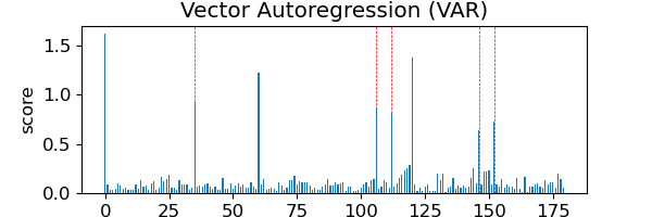
Auto-regressive (AR) models: AR models forecast future data values based on a weighted sum of past observations. We evaluate a univariate method autoregressive integrated moving average (ARIMA) with hyperparameters $(p,d,q)=(5,1,0)$, and a multivariate method vector auto-regression (VAR) with $(maxlags,differencing)=(5,1)$.

Density/neighborhood-based models: We evaluate both the local outlier factor (LOF) and Parzen window estimator (also known as kernel density estimation) which are two well-known neighborhood-based anomaly detection methods. LOF identifies anomalous data points that have a substantially lower density than their neighbors. The Parzen window estimator learns the probability density of every training data point using a kernel function. In our experiments, LOF has $n_{neighbor}=3$ and the Parzen model uses a Gaussian kernel. To obtain good estimators in these approaches, the model needs to fit on a representative data set. So, we fit the models on our training set with 10 topologies and then evaluate them on the validation set which contains data from 3 unseen topologies.

Classification models: We evaluate the one-class support vector machine (One-class SVM) model which is an unsupervised classifier to detect point outliers. It finds a decision boundary that separates high density of points (normal data) from those with small (anomalies). In our experiment, the model is trained with the RBF kernel and the upper bound on the fraction of training errors $\mu=0.5$. Then it is evaluated on the validation set.

Ensemble models: We implement an isolation forest which ensembles 100 trees, each drawing 1 feature from training data. And then, the model is evaluated on our validation set.

Topology-aware methods: We implement the DynWatch model proposed in (Li et al., 2021) which is an unsupervised time series online algorithm to detect point outliers on dynamic graphs. The model considers the impact of topology change using power sensitivity-based graph-distances.

Key findings: Table 1 contains the anomaly scores produced by different families of methods. As results show that on a dynamic graph, the online implementation of the hypothesis test method GESD gives false positive (FP) outcomes. Univariate and multivariate auto-regression models suffer from similar false positive issues when the system shifts to a new topology. Density-based, classification-based, and isolation forests need to be fitted on a set of representative data before they can be used for inference. These methods do not model topology, and thus bad estimates appear when they are used on unseen data drawn from a different topology. And the more the new topology is different from the training data, the worse the estimates are. By contrast, the topology-aware method can detect anomalies on dynamic graphs without generalization issues.

Main conclusion: ML models ignoring topology cannot adapt to dynamic graphs. Potential risks for anomaly detection include producing false positive outcomes upon any normal topology change, as well as producing bad anomaly scores on unseen data from a new topology. For application on dynamic graphs, ML models need to be topology-aware.

Due to the limited availability of real data, many ML works are trained and evaluated on synthetic data. The realistic load behaviors have shown the spatial differences among individual loads, characterized by the different peak hours and diverse styles of variation. Such patterns in load variations are neglected in many works, leading to the generation of data in an unrealistic way. As a result, a data-driven model trained and evaluated on unrealistic data can inevitably suffer from a lack of performance guarantees for practical use, raising the fear of making wrong decisions or infeasible predictions. In this section, we evaluate the risk of generalization regarding the nonconsideration of spatial load differences, from the perspective of anomaly detection and data-driven AC-OPF.

In this Section, we evaluate how anomaly detection performance can be affected when large load variations and large spatial differences in load occur. Specifically, we compare the anomaly scores using voltage and current measurement data observed from a system with varying topology and different load patterns:

• •

  Small load change and no spatial load difference: At any time, all loads in the system are assumed to have strong correlations such that all loads ramp up and down at the same rate, without differences. The load variation is created from the real load traces in the public Lawrence Berkeley National Laboratory (LBNL) load data. Appendix A.1 describes the data generation.

• •

  Load with large variation, spatial difference, and different styles: This represents a more realistic individual load pattern. The system loads are divided into different groups, each containing a subset of loads with a certain style selected from the 4 observed styles in Figure 4. Then load profiles are generated by interpolating the real-world individual load traces in the utility-provided data described in Section 2. Figure 7(b) shows the time-series data with realistic load patterns. The resulting data have large spatial differences and large load variations.

The experiment settings remain the same as Section 3.1

Key findings: The last column in Table 1 shows the anomaly detection performance of different ML models on dynamic graphs with spatial load differences. By comparison, we can see that when facing large variations and spatial differences in load, anomaly detectors tend to create more false positive outputs. For models that require fitting on some train data, the fitted model cannot generalize well to unseen load configurations, creating bad anomaly scores that make anomalies less detectable.

Main conclusion: ML models for anomaly detection can face generalization risks under large load variations and spatial load differences, producing more false positive outcomes and bad anomaly scores on unseen data. For better generalization, anomaly detection models need to build a tolerance to normal load variations.

Considering the computational complexity of obtaining a large amount of labeled data for ACOPF, we evaluate a physics-constrained neural network(Donti et al., 2021)(Li et al., [n. d.]). Unlike a supervised neural network (NN) which directly learns the input-output mapping from labeled data, the constrained neural network enables an unsupervised learning of solutions to nonlinear optimization problems, by enforcing network constraints on the output of NN. And the feasibility can be further enhanced by training with homotopy-based meta-optimization heuristics (Li et al., [n. d.]).

Now, suppose we have a series of $N_{real}$ realistic system configurations. The realistic data comes from a power grid which can be divided into several sub-networks. Each sub-network contains a group of loads with the same individual load style (e.g., all loads are heavy industrial loads that correspond to a stable constant load style) and no spatial difference between them (all loads ramp up and down at the same rate). Whereas loads from different sub-networks have spatial differences, with different various styles and peak hours. However, suppose that such a small dataset is insufficient, and we deploy data augmentation to create fake data. Specifically, a subset of these realistic data is extracted as test samples, and the remaining data are augmented to create the training and validation set. The training and implementation of the neural network model are the same as that in (Li et al., [n. d.]). Now we compare 3 different ways of data generation (see detailed setting in Appendix A.2:

• •

  naive: At any time moment, all loads are positively correlated and there is no spatial difference between individual load patterns.

• •

  grouped: At any moment, loads are divided into groups. Intra-group loads are correlated and inter-group loads have (random) spatial differences.

• •

  brute-force: every individual load has its own pattern. Random spatial differences exist everywhere.

Figure 8 compares the risk of generalization in different data generation strategies, with different $N_{fake}$. The risk of generalization is quantified by the infeasibility of NN outputs, characterized by the mean violation of network constraints. We repeat the experiments 10 times with different random seeds $0,10,20,...,90$ in data generation in order to draw reliable conclusions.

Key findings: Results in Figure 8 and Figure 9 show that the naive method which does not consider the spatial difference in data generation, results in models with poorest performance, giving highly infeasible outcomes; the grouped method has resulted in a lower risk of generalization; and the brute-force method which creates the most spatial difference in training data results in the lowest generalization risk on unseen data with realistic load patterns.

Main conclusion: ML models trained and evaluated on unrealistic data ignoring individual load differences cannot generalize well on unseen system configurations with realistic load patterns. Such risk of generalization can result in highly infeasible predictions.