Power Fluctuations of An Irreversible Quantum Otto Engine

The second law of thermodynamics tells us that any heat engines working between a hot and a cold thermal bath of constant inverse temperatures $\beta_{h}$ and $\beta_{c}$ (with $\beta=1/T$ and $k_{B}\equiv 1$) are not able to run more efficiently than a reversible Carnot cycle with its efficiency $\eta_{C}=1-\beta_{h}/\beta_{c}$. When a cyclic heat engine runs at a Carnot efficiency, its cycle operation consisting of consecutive thermodynamic processes must be reversible and thus the power output becomes null. Practically heat engines must proceed in a finite time period accounting for irreversibility and produce finite power output 1 ; 2 ; 3 ; 4 ; 5 ; 6 . The performance in finite time was intensively studied for both quantum7 ; 8 and classical4 engines. For an adequate description of heat engines, the effects induced by finite-time cycle operation on the machine performance have to be considered by involving both heat-transfer and adiabatic processes.

Unlike in macroscopic systems where both work and heat are deterministic, the work 9 ; 10 ; 11 ; 12 ; 13 ; 14 ; 15 ; 16 ; 17 and heat 18 ; 19 ; 20 for microscale systems are random due to thermal and quantum fluctuations8 ; 10 ; 21 ; 22 ; 23 ; 24 . The statistics of either work or efficiency for heat engines at microscale were examined experimentally and theoretically8 ; 16 ; 22 ; 23 ; 25 ; 26 ; 27 ; 28 ; 29 ; 30 ; 31 ; 32 ; 33 ; 34 , but under the assumption that either adiabatic8 ; 23 or isothermal strokes22 are reversible. To our knowledge, the power fluctuations have not been examined so far for an irreversible quantum heat engine where the isothermal and adiabatic strokes are finite-time and thus both of them are away from reversible limit.

In this paper, we derive the general expression for the distribution function of quantum work and heat along irreversible quantum Otto engines composed of two finite-time isochoric and two driving strokes8 ; 22 ; 23 ; 34 ; 35 ; 36 ; 37 ; 38 . This distribution function allows us to obtain the quantum work statistics explicitly depending on the time evolution dynamics of the two isochoric and two driving processes. We then analytically examine the power statistics of an Otto cycle working with an exactly, solvable two-level system. The effects of irreversibility induced by finite-time duration of either driving or isochoric strokes on machine performance and power statistics are discussed. We finally demonstrate that irreversibility results in deterioration of efficiency and power but increasing the power fluctuations, thereby indicating that the price for improving machine efficiency is increasing power fluctuations.

The model of a quantum Otto engine is sketched in Fig. 1. This machine consists of two isochoric branches, one with a hot and another with a cold thermal bath where the system frequency is kept constant, and two driving strokes, where the system (which is isolated from the two heat reservoirs and driven by the external field) undergoes unitary transformation. The four branches can be described as follows.

During the adiabatic compression $A\rightarrow B$, the system is isolated from the two thermal baths but driven by the external field, and it undergoes a unitary expansion from time $t=0$ to $t=\tau_{ch}$. Initially, the system of inverse temperature $\beta_{A}$ is assumed to be (local) thermal equilibrium 2 ; 3 , which means that the thermal occupation probability at instant $A$ takes the canonical form

$$p_{n}^{0}=\frac{e^{-\beta_{A}E^{c}_{n}}}{Z_{A}},$$

(1)

with the partition function $Z_{A}=\sum_{n}e^{-\beta_{A}E_{n}^{c}}$. The transition probability from eigenstate $|n\rangle$ to $|m\rangle$ is given by

$$p_{n\rightarrow m}^{\tau_{ch}}=|\langle n|U_{\mathrm{com}}|m\rangle|^{2},$$

(2)

where $U_{\mathrm{com}}$ denotes the unitary time evolution operator along the compression. In the special case when the system Hamiltonian evolves slowly enough by satisfying quantum adiabatic condition 38 , the system remains in the same state and the transition probability becomes $p_{n\rightarrow m}^{\tau_{ch}}=\delta_{nm}$, with the Kronecker delta function $\delta$.

The next step is the hot isochore $B\rightarrow C$, where the system with constant frequency $\omega=\omega_{h}$ is in contact with the hot thermal bath in a time duration $\tau_{h}$. The probability density of the stochastic heat absorbed from the hot bath can be determined by the conditional probability to obtain

$$p(q_{h})=\sum_{k,l}\delta[q_{h}-(E_{l}^{h}-E_{k}^{h})]p_{k\rightarrow l}^{\tau_{h}}.$$

(3)

After this system-bath interaction interval, the system is assumed to be at the local thermal equilibrium state of inverse temperature $\beta_{C}(\geq\beta_{h})$, which means that $p_{k\rightarrow l}^{\tau_{h}}={e^{-\beta_{C}E^{h}_{l}}}/{Z_{C}}$ with partition function $Z_{C}=\sum_{l}{e^{-\beta_{C}E^{h}_{l}}}$.

During the expansion $C\rightarrow D$, the system is isolated from these two thermal baths in a time period $\tau_{hc}$ while its frequency changes back to $\omega_{c}$ from $\omega_{h}$. Like in the driving compression, there is a transition probability from initial state $i$ to final one $j$, which reads

$$p_{i\rightarrow j}^{\tau_{hc}}=|\langle i|U_{\mathrm{exp}}|j\rangle|^{2},$$

(4)

where $U_{\mathrm{exp}}$ is the time evolution operator along the expansion. At the initial instant $C$ the system approaches the thermal equilibrium and the occupation probabilities take the form $p_{i}^{\tau_{ch}+\tau_{h}}=\delta_{il}p_{k\rightarrow l}^{\tau_{h}}$, where $p_{k\rightarrow l}^{\tau_{h}}$ was defined in Eq. (3).

On the fourth branch $D\rightarrow A$, the system with constant frequency $\omega=\omega_{c}$ is coupled to a cold reservoir of inverse temperature $\beta_{c}$ in a time period $\tau_{c}$. After a cycle with the total period $\tau_{cyc}=\tau_{ch}+\tau_{h}+\tau_{hc}+\tau_{c}$ the system returns to its initial state $A$, we can easily determine the quantum heat $q_{c}$ similar to that of the quantum heat $q_{h}$. As emphasized, at instant $A$ the system tends to be (local) thermal equilibrium after system-bath interaction interval, which is consistent with the assumption of canonical form Eq. (1).

In view of the fact that the work per cycle is produced only in the two driving strokes $A\rightarrow B$ and $C\rightarrow D$, the quantum work output can be obtained by determining the total work produced along these two microscopic trajectories to arrive at

$$\mathrm{w}[n(0)\rightarrow m(\tau_{ch});i(\tau_{ch}+\tau_{h})\rightarrow j(\tau_{cyc}-\tau_{c})]=(E_{i}^{h}-E_{j}^{c})-(E_{m}^{h}-E_{n}^{c}),$$

(5)

where $E_{n}^{c}$ and $E_{m}^{h}$ ($E_{i}^{h}$ and $E_{j}^{c}$) denote the respective energy eigenvalues at the initial and final instants of the compression (expansion). Here $n(t)$ are quantum numbers indicating the states occupied by the system at time $t$.

The states $|n(0)\rangle$ and $|m(\tau_{ch})\rangle$ can be assumed to be independent of $i(\tau_{ch}+\tau_{h})$ and $j(\tau_{cyc}-\tau_{c})$, since the system would relax to thermal equilibrium in an isochoric process if its time duration is long enough. This leads to the main result of this paper, namely, the following expression for the probability density of the work $\mathrm{w}$:

$$p(\mathrm{w})=\sum_{m,n,i,j}p_{n\rightarrow m}^{\tau_{ch}}p_{n}^{0}p_{i\rightarrow j}^{\tau_{hc}}p_{i}^{\tau_{ch}+\tau_{h}}\delta\{\mathrm{w}-\mathrm{w}[n(0)\rightarrow m(\tau_{ch});i(\tau_{ch}+\tau_{h})\rightarrow j(\tau_{cyc}-\tau_{c})]\},$$

(6)

where $p_{n\rightarrow m}^{\tau_{ch}}$ and $p_{i\rightarrow j}^{\tau_{hc}}$ were defined in Eq. (2) and Eq. (4), respectively. The probability distribution function Eq. (6) for the irreversible Otto engine allows us to determine all moments of quantum work: $\langle\mathrm{w}^{k}\rangle=\int\mathrm{w}^{k}p(\mathrm{w})d\mathrm{w}$ ($k=1,2,\dots).$ This result reduces to that previously obtained in a quasistatic 27 or an endoreversible 8 Otto engine when $\xi\rightarrow 0$ or $\tau_{c,h}\rightarrow\infty$. We present it here in a broader context by arguing that irreversibility is unavoidable in a finite-time cyclic engine where both the driving and system-bath interaction steps are away from quasistatic limit. For an endoreversible model where the two driving strokes are isentropic, we recover the work fluctuations 8 by setting $p_{n\rightarrow m}^{\tau_{ch}}=\delta_{nm}$ and $p_{i\rightarrow j}^{\tau_{hc}}=\delta_{ij}$, $p(\mathrm{w})=\sum_{n,i}p_{n}^{0}p_{i}^{\tau_{ch}+\tau_{h}}\delta\{\mathrm{w}-\mathrm{w}[n(0);i(\tau_{ch}+\tau_{h})]\}$.

We now consider a quantum Otto engine that works with a two-level system of the eigenenergies $E_{+}=\hbar\omega/2$ and $E_{-}=-\hbar\omega/2$. As the occupation probabilities at these two eigenstates $p_{+}=e^{-\beta\hbar\omega_{c}/2}/Z_{A}$ and $p_{-}=e^{\beta\hbar\omega_{c}/2}/Z_{A}$, where the partition function $Z_{A}=e^{-\beta_{A}\hbar\omega_{c}/2}+e^{\beta_{A}\hbar\omega_{c}/2}=2\cosh\left(\frac{\beta_{A}\hbar\omega_{c}}{2}\right),$ the mean population at instant $A$ (with time $t=0$) can be determined by using $\langle n\rangle=\sum_{n}np_{n}$ to arrive at

$$\langle n(0)\rangle=-\frac{1}{2}\tanh\left(\frac{\beta_{A}\hbar\omega_{c}}{2}\right).$$

(7)

The mean population at final instant $B$ can then be determined according to $\langle n(\tau_{ch})\rangle=\sum_{n,m}np_{m\rightarrow n}^{\tau_{ch}}p_{m}^{0}$, which together with Eqs. (1) and (2), leads to

$$\langle n(\tau_{ch})\rangle=\left(1-2\xi\right)\langle n(0)\rangle,$$

(8)

where $\xi=|\langle\pm|U_{\mathrm{com}}|\mp\rangle|^{2}$. Using $\langle n(\tau_{cyc}-\tau_{c})\rangle=\sum_{n,m}np_{m\rightarrow n}^{\tau_{hc}}p_{m}^{\tau_{ch}+\tau_{h}}$, for the unitary expansion $C\rightarrow D$ there is the relation:

$$\langle n(\tau_{cyc}-\tau_{c})\rangle=(1-2\xi)\langle n(\tau_{ch}+\tau_{h})\rangle,$$

(9)

where we have assumed $\xi=|\langle\pm|U_{\mathrm{exp}}|\mp\rangle|^{2}=|\langle\pm|U_{\mathrm{com}}|\mp\rangle|^{2}$. $\xi$ is called the adiabaticity parameter representing the probability of transition between state $|+\rangle$ and $|-\rangle$ during the compression or expansion, and the probability of no state transition is accordingly $|\langle\pm|U_{\mathrm{exp}}|\pm\rangle|^{2}=|\langle\pm|U_{\mathrm{com}}|\pm\rangle|^{2}=1-\xi$. Since the population $\langle n\rangle$ at any instant along the cycle is negative, $\xi$ must be situated between $0\leq\xi<1/2$. The adiabaticity parameter $\xi$ depends on the speed at which the driving process is performed7 ; 22 ; 36 , and it is thus a monotonic decreasing function of time duration $\tau_{h,c}$. Unlike in an adiabatic phase where the time scale of state change must be much larger than the dynamical one and the probability of state change is vanishing ($\xi=0$), during the nonadiabatic driving stroke the rapid change in frequency $\omega$ leads to inner friction and results in possible state transitions ($\xi>0$)22 ; 36 ; 39 ; 40 ; 41 ; 42 . Such nonadiabatic internal dissipation accounts for irreversible entropy production and an increase in mean population $\langle n\rangle$ (see Fig. 1).

We are interested in the finite-time operation of the Otto engine in which the isochoric processes are far away from quasistatic limit and complete thermalization can thus not be achieved for the system. Using the master equation of stochastic thermodynamics , one can find that the mean populations $\langle n(0)\rangle$ and $\langle n(\tau_{ch}+\tau_{h})\rangle$ can be expressed in terms of the corresponding asymptotic equilibrium values $\langle n_{c}\rangle^{eq}$ and $\langle n_{h}\rangle^{eq}$ (see Appendix A),

$$\langle n(0)\rangle=\langle n_{c}\rangle^{eq}+[\langle n(\tau_{cyc})\rangle-\langle n_{c}\rangle^{eq}]e^{-\gamma_{c}\tau_{c}},$$

(10)

$$\langle n(\tau_{ch}+\tau_{h})\rangle=\langle n_{h}\rangle^{eq}+[\langle n(\tau_{ch})\rangle-\langle n_{h}\rangle^{eq}]e^{-\gamma_{h}\tau_{h}}.$$

(11)

Using Eqs. (8),(9),(10) and (11), $\langle n(0)\rangle$ and $\langle n(\tau_{ch}+\tau_{h})\rangle$ can be rewritten as

$$\langle n(0)\rangle=\langle n_{c}\rangle^{eq}+\Delta_{c},\langle n(\tau_{ch}+\tau_{h})\rangle=\langle n_{h}\rangle^{eq}+\Delta_{h}$$

(12)

where

$$\Delta_{h}=\frac{\left(2\xi-1\right)\left[\left(2\xi-1\right)\langle n_{h}\rangle^{eq}+\langle n_{c}\rangle^{eq}\right]-x_{c}\left[\langle n_{h}\rangle^{eq}+\left(2\xi-1\right)\langle n_{c}\rangle^{eq}\right]}{x_{h}x_{c}-\left(2\xi-1\right)^{2}},$$

(13)

$$\Delta_{c}=\frac{\left(2\xi-1\right)\left[\left(2\xi-1\right)\langle n_{c}\rangle^{eq}+\langle n_{h}\rangle^{eq}\right]-x_{h}\left[\langle n_{c}\rangle^{eq}+\left(2\xi-1\right)\langle n_{h}\rangle^{eq}\right]}{x_{h}x_{c}-\left(2\xi-1\right)^{2}}.$$

(14)

Here $x_{h}\equiv e^{\gamma_{h}\tau_{h}}$ and $x_{c}\equiv e^{\gamma_{c}\tau_{c}}$ denote the effective time durations along the hot and cold isochoric branches, respectively. Here $\langle n_{c}\rangle^{eq}$ and $\langle n_{h}\rangle^{eq}$ are achieved in the reversible, quasistatic limit when $x_{h},x_{c}\rightarrow\infty$ leads to $\Delta_{h,c}\rightarrow 0$, whether $\xi$ is zero or not. However, $\Delta_{c}$ and $\Delta_{h}$ are still positive for finite values of $x_{c}$ and $x_{h}$ even for two reversible driving processes with $\xi\rightarrow 0$. These corrections $\Delta_{c}$ and $\Delta_{h}$ indicate that how far the heat-transfer processes deviate from the reversible limit, and imply that irreversibility is exclusively caused by heat transferred between the system and the thermal bath. Such a deviation is quite natural in both quantum heat engines and classical context when the heat-transfer processes are irreversible due to finite-time duration.

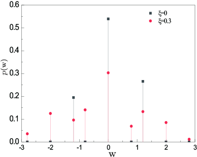
For this two-level engine, the probability density of quantum work Eq. (6) can be analytically obtained as,

	$\displaystyle p(\mathrm{w})=$	$\displaystyle\left[\frac{1}{2}+2\langle n(0)\rangle\langle n(\tau_{ch}+\tau_{h})\left(1-2\xi\right)-\left(1-\xi\right)\xi\right]\delta(\mathrm{w})$		(15)
		$\displaystyle+\frac{1}{2}\left[\left(1-2\langle n(0)\rangle\right)\left(1-\xi\right)\xi\right]\delta(\mathrm{w}+\hbar\omega_{c})$
		$\displaystyle+\frac{1}{2}\left[\left(2\langle n(\tau_{ch}+\tau_{h})\rangle+1\right)\left(1-\xi\right)\xi\right]\delta(\mathrm{w}-\hbar\omega_{h})$
		$\displaystyle+\frac{1}{4}\left[\left(2\langle n(\tau_{ch}+\tau_{h})\rangle-1\right)\left(2\langle n(0)\rangle-1\right)\xi^{2}\right]\delta(\mathrm{w}+\hbar\omega_{h}+\hbar\omega_{c})$
		$\displaystyle+\frac{1}{4}\left[1-\left(2\langle n(\tau_{ch}+\tau_{h})\rangle\right)\left(2\langle n(0)\rangle+1\right)\left(1-\xi\right)^{2}\right]\delta(\mathrm{w}+\hbar\omega_{h}-\hbar\omega_{c})$
		$\displaystyle+\frac{1}{4}\left[\left(2\langle n(\tau_{ch}+\tau_{h})\rangle+1\right)\left(1-2\langle n(0)\rangle\right)\left(1-\xi\right)^{2}\right]\delta(\mathrm{w}+\hbar\omega_{c}-\hbar\omega_{h})$
		$\displaystyle+\frac{1}{2}\left[\left(2\langle n(0)\rangle+1\right)\left(1-\xi\right)\xi\right]\delta(\mathrm{w}-\hbar\omega_{c})$
		$\displaystyle+\frac{1}{4}\left[\left(2\langle n(0)\rangle+1\right)\left(2\langle n(\tau_{ch}+\tau_{h})\rangle+1\right)\xi^{2}\right]\delta(\mathrm{w}-\hbar\omega_{c}-\hbar\omega_{h})$
		$\displaystyle+\frac{1}{2}\left[\left(1-2\langle n(\tau_{ch}+\tau_{h})\rangle\right)\left(1-\xi\right)\xi\right]\delta(\mathrm{w}+\hbar\omega_{h}).$

The stochastic work can take nine different discrete values as shown Fig. 2. The following should be noted in respect of the stochastic work per cycle: (i) $\mathrm{w}=0$ indicates that the stochastic work by the system along the expansion is fully counterbalanced by that during the compression. (ii) $\mathrm{w}=\hbar\omega_{c}-\hbar\omega_{h}$ ($\mathrm{w}=\hbar\omega_{h}-\hbar\omega_{c}$) corresponds to the case when the system jumps down from high-energy (low-energy) state to low-energy (high-energy) one along the hot isochore, namely, $n=m=1/2$ but $i=j=-1/2$ ( $n=m=-1/2$ and $i=j=1/2$) in Eq. (6). These values exist in the adiabatic or nonadiabatic driving. (iii) There are more values of stochastic work in the nonadiabatic driving than in the adiabatic case due to quantum fluctuations induced by nonadiabatic transitions. (iv) Finally the distribution $p(\mathrm{w})$ is expected to be normalized to one either for adiabatic or nonadiabatic driving.

Using Eq. (3), the average heat injection, $\langle q_{h}\rangle=\int q_{h}p(q_{h})dq_{h}$, can be obtained as

$$\langle q_{h}\rangle=\hbar\omega_{h}[\langle n(\tau_{ch}+\tau_{h})\rangle-(1-2\xi)\langle n(0)\rangle].$$

(16)

By using simple algebra (see Appendix B for details), the average work ($\langle\mathrm{w}\rangle$) and the work fluctuations ($\delta\mathrm{w}^{2}=\langle\mathrm{w}^{2}\rangle-\langle\mathrm{w}\rangle^{2}$) can be obtained as

$$\langle\mathrm{w}\rangle=\hbar[\omega_{c}-(1-2\xi)\omega_{h}]\langle n(0)\rangle+\hbar[\omega_{h}-(1-2\xi)\omega_{c}]\langle n(\tau_{ch}+\tau_{h})\rangle,$$

(17)

and

	$\displaystyle\delta\mathrm{w}^{2}=$	$\displaystyle\hbar^{2}\omega_{h}^{2}[\frac{1}{2}-\langle n(0)\rangle^{2}(1-2\xi)^{2}-\langle n(\tau_{ch}+\tau_{h})\rangle^{2}]$		(18)
		$\displaystyle+\hbar^{2}\omega_{c}^{2}[\frac{1}{2}-\langle n(0)\rangle^{2}-(1-2\xi)^{2}\langle n(\tau_{ch}+\tau_{h})\rangle^{2}]$
		$\displaystyle-\hbar^{2}\omega_{c}\omega_{h}(1-2\xi)[1-2\langle n(0)\rangle^{2}-2\langle n(\tau_{ch}+\tau_{h})\rangle^{2}].$

From Eqs. (16) and (17), the machine efficiency defined by $\eta=\langle\mathrm{w}\rangle/\langle q_{h}\rangle$, can be expressed as

$$\eta=1-\frac{\omega_{c}}{\omega_{h}}\frac{\langle n(0)\rangle-(1-2\xi)\langle n(\tau_{ch}+\tau_{h})\rangle}{(1-2\xi)\langle n(0)\rangle-\langle n(\tau_{ch}+\tau_{h})\rangle}.$$

(19)

In case both isochoric and driving processes proceed in finite time, internal dissipation and uncomplete thermalization occur in the system resulting in the thermodynamic efficiency Eq. (19) that depends on the time evolution along each cycle except if these four processes may be done infinitely long, making the efficiency reduce to the one for cycles with complete thermalization, $\eta=1-\frac{\omega_{c}}{\omega_{h}}\frac{(1-2\xi)\langle n_{h}\rangle^{eq}-\langle n_{c}\rangle^{eq}}{\langle n_{h}\rangle^{eq}-(1-2\xi)\langle n_{c}\rangle^{eq}}$7 ; 34 ; 36 , or the one for models without internal dissipation 2 ; 3 ; 35 , $\eta=1-\frac{\omega_{c}}{\omega_{h}}$.

The efficiency and work fluctuations as a function of the inverse temperature $\beta_{c}$ of cold bath is shown in Fig. 3(a) and Fig. 3(b). When increasing temperature, the efficiency $\eta$ increases but the work fluctuations $\delta\mathrm{w}^{2}$ decrease. The efficiency at high temperatures is larger than that at low temperatures, showing that the quantum effects which are of significance in low temperature regime can improve the machine efficiency. Because the quantum fluctuations characterizing the low temperature domain are smaller than the thermal fluctuations dominating the high temperature region, the work fluctuations $\delta\mathrm{w}^{2}$ get increased while the temperature is increased and vice versa. The increase in the adiabacity parameter $\xi$ yields in a decrease (an increase) in the machine efficiency (work fluctuations) as it should, thereby showing that there is a trade-off between efficiency and work fluctuations.

Since the stochastic power is the work divided by the cycle period $\tau_{cyc}$, namely, $\dot{\mathrm{w}}[|n(0)\rangle;|n(\tau_{ch}+\tau_{h})\rangle]=\mathrm{w}[|n(0)\rangle;|n(\tau_{ch}+\tau_{h})\rangle]/\tau_{cyc}$, the relative fluctuations of the power $f_{\dot{\mathrm{w}}}$ are equivalent to corresponding those of work $f_{\mathrm{w}}$, leading to $f_{\dot{\mathrm{w}}}=f_{\mathrm{w}}=\sqrt{\delta\mathrm{w}^{2}}/\langle\mathrm{w}\rangle$. For nonadiabatic driving branches, the relative power fluctuations are increasing with decreasing effective time durations $x_{c}$ and $x_{h}$, see Fig. 4(a) and Fig. 4(b). Comparison between these two figures shows that irreversible nonadiabatic friction related to $\xi$, which is a monotonic decreasing function of $\tau_{h}$ as well as $\tau_{c}$, leads to an increase in relative power fluctuations. This can be understood by the fact that irreversibility either induced by finite heat flux between the system and the bath or caused by internal irreversible dissipation yields larger fluctuations than those in the reversible cycle operation. In view of the fact that the power is a monotonic decreasing function of time durations $\tau_{h}$ and $\tau_{c}$, we see that the price one should pay for increasing power is increasing power fluctuations.

In summary, we derived the probability distribution of stochastic work of quantum Otto engines working within a cycle period of finite time that leads to irreversibility in both the two isochoric and two driving processes. Employing a two-level system as the working substance of these engines, we find that, although the average work is positive, the quantum work may be negative due to quantum indeterminacy. Afterwards, we derived the analytical expressions for the power output, efficiency, and work fluctuations, all of which are dependent on the time allocations the four thermodynamic processes. We finally determined statistics of work as well as power at any finite temperatures, and showed that there is a trade-off between efficiency (or power) and power fluctuations.

References

- (1) D. Gauthier, Phys. World 18, 30 (2005).
- (2) T. Feldmann, and R. Kosloff, Phys. Rev. E 68, 016101 (2003); T. Feldmann, and R. Kosloff, Phys. Rev. E 61, 4774 (2000).
- (3) Y. Rezek, and R. Kosloff, New J. Phys. 8, 83 (2006).
- (4) Z. C. Tu, Chin. Phys. B 21, 020513 (2012).
- (5) Z. C. Tu, J. Phys. A 41, 312003 (2008).
- (6) F. Wu , L. G. Chen, F. R. Sun, C. Wu, and Q. Li, Phys. Rev. E 73, 016103 (2006).
- (7) O. Abah, J. Roßnagel, G. Jacob, S. Deffner, F. Schmidt-Kaler, K. Singer, and E. Lutz, Phys. Rev. Lett. 109, 203006 (2012).
- (8) Y. Hong, Y. Xiao, J. He, and J. H. Wang, Phys. Rev. E 102, 022143 (2020).
- (9) B. Gaveau, M. Moreau, and L. S. Schulman, Phys. Rev. Lett. 105, 060601 (2010).
- (10) G. Maslennikov, S. Ding, R. Hablützel, J. Gan, A. Roulet, S. Nimmrichter, J. Dai, V. Scarani, and D. Matsukevich, Nat. Commun. 10, 202 (2019).
- (11) G. Verley, C. V. D. Broeck, and M. Esposito, New J. Phys. 16, 095001 (2014).
- (12) P. Solinas, D. V. Averin, and J. P. Pekola, Phys. Rev. B 87, 060508(R) (2013).
- (13) Y. Qian, and F.Liu, Phys. Rev. E 100, 062119 (2019).
- (14) P. Talkner, E. Lutz, and P. Hänggi, Phys. Rev. E 75, 050102 (2007).
- (15) Z. Fei, N. Freitas, V. Cavina, H. T. Quan, and M. Esposito, Phys. Rev. Lett. 124, 170603 (2020).
- (16) F. Cerisola, Y. Margalit, S. Machluf, A. J. Roncaglia, J. P. Paz, and R. Folman, Nat. Commun. 8, 1241 (2017).
- (17) F. W. J. Hekking, and J. P. Pekola, Phys. Rev. Lett. 111, 093602 (2013).
- (18) S. Rahav, U. Harbola, and S. Mukamel, Phys. Rev. A 86, 043843 (2012).
- (19) T. Denzler, and E. Lutz, Phys. Rev. E 98, 052106 (2018).
- (20) S. Gasparinetti, P. Solinas, A. Braggio, and M. Sassetti, New J. Phys. 16, 115001 (2014).
- (21) U. Seifert, Rep. Prog. Phys. 75, 126001 (2012).
- (22) T. Denzler, and E. Lutz, Phys. Rev. Research 2, 032062 (2020).
- (23) J. H. Wang, J. Z. He, and Y. L. Ma, Phys. Rev. E 100, 052126 (2019).
- (24) M. Esposito, U. Harbola, and S. Mukamel, Rev. Mod. Phys. 81, 1665 (2009).
- (25) V. Holubec, and A. Ryabov, Phys. Rev. Lett. 121, 120601 (2018).
- (26) V. Holubec, J. Stat. Mech. P05022, (2014).
- (27) V. Holubec, and A. Ryabov, Phys. Rev. E 96, 030102 (2017).
- (28) H. Vroylandt, M. Esposito, and G. Verley, Phys. Rev. Lett. 124, 250603 (2020).
- (29) J. M. Park, H. M. Chun, and J. D. Noh, Phys. Rev. E 94, 012127 (2016).
- (30) J. H. Jiang, B. K. Agarwalla, and D. Segal, Phys. Rev. Lett. 115, 040601 (2015).
- (31) H. Vroylandt, A. Bonfils, and G. Verley, Phys. Rev. E 93, 052123 (2016).
- (32) G. Verley, and M. Esposito, Phys. Rev. Lett. 114, 050601 (2015).
- (33) G. Verley, T. Willaert, C. V. D. Broeck, and M. Esposito, Phys. Rev. E 90, 052145 (2014).
- (34) J. P. S. Peterson, T. B. Batalhão, M. Herrera, A. M. Souza, R. S. Sarthour, I. S. Oliveira, and R. M. Serra, Phys. Rev. Lett. 123, 240601 (2019).
- (35) F. L. Wu, J. Z. He, Y. L. Ma, and J. H. Wang, Phys. Rev. E 90, 062134 (2014).
- (36) R. J. de Assis, T. M. de Mendonça, C. J. Villas-Boas, A. M. de Souza, R. S. Sarthour, I. S. Oliveira, and N. G. de Almeida, Phys. Rev. Lett. 122, 240602 (2019).
- (37) S. H. Su, X. Q. Luo, J. C. Chen, and C. P. Sun, Europhys. Lett 115, 30002 (2016).
- (38) M. Born, and V. Fock, Z. Phys. 51, 165 (1928).
- (39) A. Alecce, F. Galve, N. L. Gullo, L. Dell'Anna, F.Plastina, and R. Zambrini, New J. Phys. 17, 075007 (2015).
- (40) S. Lee, M. Ha, Jong-Min Park, and H. Jeong, Phys. Rev. E 101, 022127 (2020).
- (41) F. Plastina, A. Alecce, T. J. G. Apollaro, G. Falcone, G. Francica, F. Galve, N. Lo Gullo, and R. Zambrini, Phys. Rev. Lett. 113, 260601 (2014).
- (42) L. A. Correa, J. P. Palao, and D. Alonso, Phys. Rev. E 92, 032136 (2015).
- (43) M. Esposito, and C. V. D. Broeck, Phys. Rev. E 82, 011143 (2010).