Power-Efficient Optimization for Coexisting Semantic and Bit-Based Users in NOMA Networks
Abstract
Semantic communication focuses on transmitting the meaning of data, aiming for efficient, relevant communication, while non-orthogonal multiple access (NOMA) enhances spectral efficiency by allowing multiple users to share the same spectrum. Integrating semantic users into a NOMA network with bit-based users improves both transmission and spectrum efficiency. However, the performance metric for semantic communication differs significantly from that of traditional communication, posing challenges in simultaneously meeting individual user demands and minimizing transmission power, especially in scenarios with coexisting semantic and bit-based users. Furthermore, the different hardware architectures of semantic and bit-based users complicate the implementation of successive interference cancellation (SIC). To address these challenges, in this paper, we propose a clustered framework to mitigate the complexity of SIC and two multiple access (MA) schemes, e.g., pure cluster-based NOMA (P-CNOMA) and hybrid cluster-based NOMA (H-CNOMA), to minimize the total transmission power. The P-CNOMA scheme can achieve the minimum transmission power, but may not satisfy the high quality of service (QoS) requirement. In contrast, H-CNOMA addresses these issues with a slight increase in power and a reduced semantic rate. These two schemes complement each other, enabling an adaptive MA selection mechanism that adapts to specific network conditions and user requirements.
Index Terms:
beamforming design, non-orthogonal multiple access (NOMA), semantic communicationI Introduction
Rapid growth in connected devices and wireless applications, such as remote healthcare (RHC) [1], virtual reality (VR), and augmented reality (AR) [2], is driving an unprecedented increase in data traffic. As multimedia technologies continue to mature, the demand for ubiquitous high-quality communication services has increased, resulting in a significant increase in the volume of data that must be transmitted. This increased data traffic has led to major challenges in wireless communication systems, especially in terms of resource scarcity and spectrum constraints. Addressing these challenges has become crucial to ensuring that future communication systems can meet user expectations. There are two main directions to overcome these challenges, which are improving resource utilization efficiency and reducing overall traffic. One efficient approach to enhance spectrum efficiency is non-orthogonal multiple access (NOMA), which allows multiple users to share the same resource block by allocating different power levels. This approach uses superposition coding at the transmitter and successive interference cancellation (SIC) at the receiver to improve spectrum efficiency [3, 4]. On the other hand, semantic communication, which focuses on conveying the intended meaning of information instead of transmitting raw data, has garnered considerable attention to reduce the amount of data and improve transmit efficiency [5, 6, 7]. Recent advances in deep learning have further empowered semantic communication, which enables the efficient processing of diverse data types, such as text, speech, images, and video [8, 9, 10, 11]. As a result, it is natural to explore the integration of semantic communication with NOMA networks motivated by these advantages.
I-A Related Works
Shannon and Weaver first introduced the concept of semantic communication in [12], 1949. After that, research on semantic communication has continued to progress steadily, such as the concept of semantic web [13] and the novel framework of semantic communication [14]. With the rapid development in artificial intelligence and machine learning in recent years, semantic communication has entered a new era. Many studies focus on improving performance, particularly in terms of semantic similarity or semantic accuracy, across various data types, including text, speech, images, and video. The authors of [15] proposed DeepSC for text transmission, which outperforms than conventional schemes. The authors of [8] extended DeepSC to a multi-user scenario for text data transmission. Then, the research shifts focus to various data types. For example, the authors of [9] presented a deep learning-enabled semantic communication system that converts speech transmission to text-related semantic features, significantly reducing data requirements while maintaining high performance, the authors of [10] proposed an end-to-end semantic communication system for efficient image transmission by implementing a deep learning-based classifier at the sender and a diffusion model at the receiver and the authors of [11] extended the method in [10] to transmit videos by converting videos into frames. Besides the above works that primarily focus on enhancing transmission performance, some works investigate semantic communication from a task-oriented perspective. For example, the authors of [16] established a multi-user semantic communication system called MU-DeepSC, which leverages correlated image and text data for the visual question answering (VQA) task. MU-DeepSC effectively processes and combines semantic information from images and text to accurately predict answers. The authors in [17] developed a semantic communication system based on deep learning that simultaneously performs image recovery and classification tasks by integrating JSCC. The system employs a novel loss function to enhance robustness and reduce communication overhead under varying channel conditions.
The aforementioned studies focus primarily on optimizing semantic communication at the structural level. Specifically, they emphasize designing innovative encoders and decoders or developing new system architectures by integrating novel components. However, since most semantic devices function within wireless communication networks, some research shifts the focus to network-level optimization. This includes adopting NOMA techniques and designing efficient resource allocation schemes to enhance overall performance. For example, recent work [18] studied the downlink scenario where the base station (BS) serves multiple semantic users by adopting NOMA. However, conventional bit communication still dominates at current stage, it is unrealistic to completely replace all bit-based devices with semantic devices. Hence, it is more worthy to investigate the practical scenario where semantic users and bit-based users co-exist. Recently, work [19] studied the simplest case where one semantic user and one traditional user simultaneously transmit data to a single antenna BS by adopting NOMA. Based on [19], the authors also proposed a semi-NOMA scheme for this case in [20].
I-B Motivations and Contributions
Given the significant performance benefits of both NOMA and semantic communication, extending the semantic-bit NOMA network to a multi-user scenario is a critical research direction. Additionally, with the growing emphasis on green communication, many applications demand systems that deliver high performance while minimizing energy consumption. Therefore, it is essential to investigate resource allocation strategies in multi-user semantic-bit NOMA networks to achieve minimal transmission power. To the best of our knowledge, no existing work has addressed resource allocation optimization in multi-user NOMA systems where semantic and bit-based users coexist. In this paper, we focus on this challenging scenario where one BS serves multiple semantic users and multiple conventional bit users simultaneously by adopting NOMA. To introduce spatial diversity, the BS is assumed to be equipped with multiple antennas, which consequently introduces more challenges. We propose a multi-cluster NOMA network to accommodate each two users into one cluster. Two MA transmission schemes are proposed: the P-CNOMA scheme and the H-CNOMA scheme. For the P-CNOMA scheme, an iteration-free algorithm is developed to efficiently solve the optimization problem. The optimization problem for the H-CNOMA scheme is reformulated as a constraint-free problem, which is effectively solved using a deep neural network.
The main contributions of this paper are summarized as follows:
-
•
We propose a multi-cluster NOMA network that groups semantic and conventional bit users into clusters, with each cluster comprising two users of the same type to take care of two different hardware architectures. SIC is applied only within each cluster, treating signals from other clusters as interference, thus significantly reducing the complexity of the SIC process. The BS, equipped with multiple antennas, simultaneously serves multiple clusters by generating a unique beam for each cluster. Within the same cluster, two users share the same beam, performing power allocation accordingly.
-
•
We develop the P-CNOMA scheme to minimize the total transmission power. The formulated problem is non-convex due to the coupling of the beamforming vector and the power allocation coefficient. Moreover, since the objective function is not directly related to the power allocation coefficient, the alternating algorithm may exhibit poor convergence performance. We propose an iteration-free algorithm to solve the problem. The formulated problem is first transformed to a problem without composite constraints 111The composite constraint in this paper refers to a constraint that can be equivalently decomposed into two or more individual constraints. For example, is equivalent to and , hence, is a composite constraint. By determining the upper and lower bounds of the power allocation coefficient, the primal problem is approximately transformed into a single-variable optimization problem. Subsequently, semi-definite relaxation (SDR) is employed to efficiently solve this problem.
-
•
We develop the H-CNOMA scheme to compensate for the shortcomings of P-CNOMA. Although the aforementioned P-CNOMA scheme can achieve the lowest transmission power, it faces feasibility issues, particularly when conventional bit users demand high data rates or when semantic users require high semantic similarity. In the H-CNOMA scheme, the primal problem can be solved on a per-cluster basis due to the absence of inter-cluster interference. It is reformulated into a constraint-free problem, and a deep neural network is introduced to efficiently find the solution. This scheme can meet the high data rate demands of bit users and the high semantic similarity requirements of semantic users with a slight increase in transmission power. However, the maximum achievable semantic rate is constrained by the use of multiple frequency sub-channels. Consequently, these two schemes complement each other, and the choice between them should be made based on specific system requirements.
-
•
The simulation results introduce the concepts of effective semantic similarity, the semantic similarity domination region, and the semantic rate domination region. We analyze the impact of these two regions on the effective semantic similarity from the simulation results. Generally, the effective semantic similarity matches the target semantic similarity when the target semantic rate falls within the similarity domination region. However, when the target semantic rate falls within the semantic rate domination region, the effective semantic similarity depends solely on the target semantic rate. Moreover, reveal how the two proposed MA schemes effectively complement one another.
I-C Organization and Notation
The rest of the paper is organized as follows. In Section II, the system model is introduced and the total transmission power minimization problem is formulated. In Section III, two schemes are proposed along with the optimization algorithms. In Section IV, simulation results are provided. Finally, a conclusion is summarized in Section V.
Notations: , and represent matrix, vector and scalar, respectively. represents the conjugate transpose of vector . represents the space of a complex vector and represents the space of a complex matrix. represents norm.
II System Model and Problem Formulation
The system model shown in Fig. 1 consists of a BS equipped with antennas, serving single-antenna semantic users (S-users) and single-antenna bit users (B-users). S-users and B-users receive signals in a semantic communication manner and a traditional communication manner, respectively. It is known that the complexity of SIC grows significantly with the number of users increasing [21]. To mitigate this, we assume that each cluster consists only of two users and that SIC is applied only within each cluster. The BS simultaneously transmits semantic and bit streams to the S-users and B-users and generates a unique beam for each cluster, with two users in the same cluster sharing the beam through different power levels.
Due to the different decoding methods employed by the two types of communication, the hardware architecture of a semantic device differs from that of a traditional device. Specifically, semantic devices are equipped with artificial intelligence (AI) chips that store pre-trained models for decoding semantic information, while traditional devices use digital signal processing (DSP) chips to decode bit information. To reduce hardware complexity, it is assumed that semantic users only decode semantic information and bit users only decode bit information. Consequently, each cluster consists of users of the same type.
The clustering strategy pairs users with the most disparate channel gains to improve SIC performance. According to previous work [22, 23], a greater disparity in channel gains between users can significantly enhance the efficiency of SIC in NOMA systems. This performance enhancement arises because SIC relies on distinguishing between user signals based on power levels. When there is a larger difference in the channel gains of the users, it becomes easier to allocate power such that one user’s signal can be decoded without interference from the other. Specifically, the user with the highest channel gain is paired with the user having the lowest channel gain, followed by pairing the second-highest user with the second-lowest channel gain user, and so on.
II-A Semantic Rate
It is critical to define the semantic rate for network-level performance optimization. In this paper, we assume the typical DeepSC text transmission system described in [24] is deployed. Let denote the average number of semantic symbols per word and denote the SNR. According to [24], semantic similarity, which describes the similarity between the recovered sentence and the original sentence in a DeepSC text transmission system, is highly related to and . The resultant expression of the semantic similarity can be a function of and , i.e., . [25] evaluated the semantic rate based on the semantic similarity, which is given by
| (1) |
where denotes the transmission bandwidth as well as the symbol rate and denotes average semantic information per sentence measured by semantic unit per second (suts). To obtain a traceable closed-form expression of the semantic similarity, [20] utilized a data regression method to approximate by a generalized logistic function. For any given , the semantic similarity can be expressed as follows:
| (2) |
where and are both positive and respectively denote the left asymptote and the right asymptote. is the logistic growth rate, affects the logistic mid-point and affects near which asymptote maximum growth occurs. Note that is monotonically increasing with , hence, we have .

II-B Problem Formulation
To reduce the complexity associated with SIC and hardware requirements, it is assumed that each cluster consists of only two users of the same type. In each cluster, which consists of either two S-users or two B-users 222It is assumed that is even, which means each type of users can be allocated into clusters., the user with the higher channel gain is referred as the strong user, while the one with the lower channel gain is referred as the weak user. In the -th S-user cluster, the strong and weak users are denoted as and , respectively. Likewise, in the -th B-user cluster, they are represented as and . and are the corresponding signals of and , while and are corresponding signals to and . The superimposed signal transmitted by the BS can be expressed as follows:
| (3) |
and represent beamforming vectors for the -th S-user cluster and -th B-user cluster, respectively. and respectively denote power allocation coefficients in the -th S-user cluster and B-user cluster. Thus, the received signal by and can be expressed as:
| (4) |
where and denote the channel vectors on the BS- link and the BS- link, respectively, and and denote the zero-mean additive white Gaussian noise (AWGN) with variance . Similarly, the received signal by and in the -th B-user cluster can be expressed as:
| (5) |
Let first consider the SIC procedure in S-user clusters. As SIC is only applied in each cluster, the decoding order is assumed to be that the strong user first decodes the weak user’s signal and then its own signal and the weak user directly decodes its own signal. During SIC, signals from users in other clusters are considered as interference. We assume the perfect channel state information (CSI) is available to all users and all signals have the unit power, satisfying with the expectation operation . For the simple notation, we define a function to express inter-cluster interference to the th S-user cluster through channel fading , which is expressed as
| (6) |
Similarly, the inter-cluster interference function of the -th B-user cluster is expressed as
| (7) |
Therefore, the signal-to-interference-plus-noise ratio (SINR) of ’s signal decoded by is given by
| (8) |
After ’s signal was successfully decoded, removes intra-cluster interference. Hence, the SNR of ’s signal is given by
| (9) |
The SNR of ’s signal decoded by itself is given by
| (10) |
Then, the achievable semantic rate of and can be expressed as
| (11) |
and
| (12) |
respectively.
The SIC procedure in B-user clusters is similar to the above. Therefore, the SINR of ’s signal decoded by is given by
| (13) |
After removing intra-cluster interference, the SNR when decodes its own signal is given by
| (14) |
As directly decodes its own signal, the SNR can be expressed as follows:
| (15) |
Then, the achievable data rate of and can be expressed as
| (16) |
and
| (17) |
respectively.
It is assumed that all S-users have the same target semantic rate and target semantic similarity , and all B-users have the same target data rate . The transmission power minimization problem can be formulated as follows:
| (18a) | ||||
| (18b) | ||||
| (18c) | ||||
| (18d) | ||||
| (18e) | ||||
| (18f) | ||||
where is a beamforming matrix collecting all beamforming vectors and is a vector collecting all power allocation coefficients. Constraint (18b) guarantees each S-user to achieve the target semantic rate. Constraint (18c) is introduced to guarantee the minimal requirement of semantic similarity. The reason to introduce constraint (18c) is that the semantic rate can be large if the transmission bandwidth is sufficiently large even the semantic similarity is small according to (1). Therefore, the semantic similarity is another critical metric to evaluate the performance of semantic communication. Constraint (18d) guarantees each B-user to achieve the target data rate and constraints (18b), (18c) and (18d) jointly guarantee a successful SIC procedure.
III Optimization Algorithms
In this section, two MA transmission schemes are proposed. The first one is P-CNOMA scheme, where each user utilizes the entire bandwidth for signal transmission, but inter-cluster interference occurs. The second one is H-CNOMA scheme, where frequency sub-channels are allocated to each cluster to cancel inter-cluster interference, though this results in reduced transmission bandwidth resources.
III-A Pure Cluster-based NOMA Transmission Scheme
It is noted that two optimization variables, the beamforming vector and the power allocation coefficient, are coupled together in . One common method to solve a multi-variable optimization problem is the alternating algorithm, where one variable is fixed and only another is optimized. However, the power allocation coefficient will not affect the objective function of directly. As a result, the alternating algorithm may have the difficulty on convergence when solving this problem. The idea is to transfer to a problem only related to beamforming and then solve it by convex optimization.
According to the definition of semantic rate, constraint (18b) can be rewritten as
| (19) |
where . It is noted that constraint (18c) and constraint (19) can be combined as one constraint, which is given by
| (20) |
where denotes the effective semantic similarity. Therefore, can be rewritten as
| (21a) | ||||
is a non-convex problem because of constraint (18d) and constraint (20). According to optimization theory, constraint (20) can be equivalently split into three sub-constraints , and , for any given . These three sub-constraints can be further recast into , and , where denotes the inverse function of (2). Similarly, constraint (18d) can be equivalently split into two sub-constraints and , which can be further rewritten as , and with . As a result, can be recast into
| (22a) | ||||
| (22b) | ||||
| (22c) | ||||
| (22d) | ||||
| (22e) | ||||
| (22f) | ||||
| (22g) | ||||
Although there is no constraint in , constraints (22b)-(22g) are non-convex. Hence, is still a NP hard problem, which is difficult to be solved in polynomial time. After the algebraic transformation, constraint (22b) can be rewritten as follows
| (23) |
From (23), a relationship between and is obtained, which is
| (24) |
Similarly, another two relationships between and can be obtained from (22c) and (22d), which are
| (25) |
and
| (26) |
Considering and , the lower bound of is given by
| (27) |
and the upper bound of is given by
| (28) |
where .
Lemma 1
always holds.
Proof.
Please refer to Appendix A. ∎
The next step is to find the lower bound and upper bound of . According to (22e)-(22g), we have
| (30) |
| (31) |
and
| (32) |
Similarly, we have the lower bound of
| (33) |
and the upper bound of
| (34) |
where . can be proved less than 1 by following the method in Lemma 1. Then, the upper bound of is
| (35) |
A feasible always exists as long as holds.
Consequently, can be recast into the following form:
| (36a) | ||||
| (36b) | ||||
| (36c) | ||||
Only beamforming vectors in need to be optimized. The next step is to deal with constraint (36b). Constraint (36b) is equivalent to the following two constraints
| (37) |
and
| (38) |
It is noted that and have the same denominator, hence, (37) can be rewritten into
| (39) |
which becomes a quadratic form. As for (38), it represents a quadratic fractional form, which has significant challenges when attempting to transform it into a convex form.
Proposition 1
Constraint (38) can be removed by assuming and .
Proof.
Please refer to Appendix B. ∎
According to Proposition 1, constraint (36b) can be replaced by constraint (39). Follow the step above, constraint (36c) can be replaced by
| (40) |
when assuming and . Then, can be recast into
| (41a) | ||||
| (41b) | ||||
| (41c) | ||||
| (41d) | ||||
| (41e) | ||||
is still non-convex due to the quadratic term. One efficient way to deal with quadratic constraint is SDR [26]. Auxiliary matrices , , , , and are introduced. By applying SDR, the trace of matrix replaces the quadratic term. For example, is replaced by and is replaced by . The inter-cluster interference function after SDR can be expressed as
| (42) |
and
| (43) |
Hence, can be recast as the following form
| (44a) | ||||
| (44b) | ||||
| (44c) | ||||
| (44d) | ||||
| (44e) | ||||
| (44f) | ||||
| (44g) | ||||
| (44h) | ||||
| (44i) | ||||
| (44j) | ||||
| (44k) | ||||
where and . To ensure is convex, we temporarily disregard the rank one constraints (44j) and (44k). As a result, we obtain a convex formulation that
| (45a) | ||||
Since the rank one constraint is disregarded in , the optimal value of might not be the optimal value of . Let and denote the optimal solution of . If and hold, it suggests the optimal solution of can be successfully recovered from and by eigen-decomposition. However, if the above equations do not hold, only the suboptimal solution of can be obtained by Gaussian Randomization.
Proposition 2
The rank of and can be guaranteed as 1.
Proof.
Please refer to Appendix B. ∎
III-B Hybrid Cluster-based NOMA Transmission Scheme
Although the aforementioned P-CNOMA scheme allows each user to fully utilize the whole spectrum and achieve the minimal transmission power, however, it has the feasibility issue that arises from the interference (6) and (7). As transmission power increases, interference power rises accordingly. Consequently, once the target QoS exceeds a certain threshold, further increases in transmission power cannot achieve the desired target. To address this issue, we propose the H-CNOMA scheme, where each cluster occupies one orthogonal frequency sub-channel, with two users within the same cluster sharing the sub-channel. In this scheme, OMA is adopted between clusters while NOMA is adopted between users within the same cluster. Due to orthogonality of sub-channels, the inter-cluster interference is eliminated, but at the cost of reduced bandwidth. Since each cluster is independent to other clusters, we can focus on a single cluster when formulating the optimization problem. Let take a S-user cluster as an example, the transmission power minimization problem can be expressed as
| (46a) | ||||
| (46b) | ||||
| (46c) | ||||
| (46d) | ||||
where and denote the semantic rates of the strong user and the weak user, respectively. The terms , and denote the SINR/SNR of the strong user’s signal, the weak user’s signal, and the weak user’s signal as decoded by the strong user, respectively. After some algebraic transformations, we have the following equations:
| (47) |
| (48) |
| (49) |
| (50) |
and
| (51) |
denotes the channel vector between the BS and the strong user and the weak user in this S-user cluster. After decoupling constraints (46b) and (46c), is recast into
| (52a) | ||||
| (52b) | ||||
| (52c) | ||||
| (52d) | ||||
| (52e) | ||||
where the effective semantic similarity It is noted that , where and . Similarly, .
Proposition 3
If is feasible, and are not orthogonal to and should be satisfied.
Proof.
Please refer to Appendix D. ∎
When the conditions in Proposition 3 are satisfied, constraints (52b) - (52d) can be rewritten as
| (53) |
| (54) |
and
| (55) |
, and are three functions related to and . The optimal value of is
| (56) |
Therefore, can be recast into
| (57a) | ||||
| (57b) | ||||
If we want to transform into an unconstrained problem, we need to remove constraint (57b). By introducing an auxiliary variable and letting
| (58) |
constraint (57b) can be eliminated. is a sigmoid function, whose output is in the range 0 to 1. It is noted that the domain of is . Finally, can be recast into
| (59a) | ||||
is unconstrained but non-convex, which can be efficiently solved by a neural network. In particular, unsupervised learning can be utilized to solve this problem. In this paper, we utilize a four-layer fully connected neural network, whose input is and and output is and . The loss function is (59a).
The method above can be also applied to minimize the transmission power in a B-user cluster. The only difference is that is replaced by . The detail is not provided due to the space limitation. Once the minimal transmission power for each cluster is determined, the total minimal transmission power of the system is obtained by summing the powers of all clusters.

It is noted that the semantic rate in this transmission scheme is also related to the number of clusters due to the introduction of frequency sub-channels. Fig. 2 illustrates the relationship between semantic similarity and semantic rate for various numbers of clusters when MHz and . It suggests that the maximum semantic rate decreases when the network accommodates more clusters. This is because the maximum semantic similarity is 1, then the maximum semantic rate is
| (60) |
which explains Fig. 2. Once the target semantic similarity is set, there are two regions named semantic similarity domination region and semantic rate domination region. If the target semantic rate is located in the semantic similarity domination region, the effective semantic similarity is always equal to the target semantic similarity , whereas if it is located in the semantic rate domination region, the effective semantic similarity is only related to the target semantic rate.
IV Simulation Results
In this section, simulation results are provided to illustrate the superior performance of the proposed transmission schemes compared with the benchmarks. In the simulation results, the first benchmark scheme, referred as ’Random P-CNOMA’, employs the same MA transmission approach as the P-CNOMA scheme. However, unlike the proposed scheme, the clustering strategy in Random P-CNOMA does not follow the channel condition order and instead clusters users randomly. The second benchmark, referred as ’Non-Cluster OMA’, does not group users into clusters. Instead, each user is assigned an orthogonal frequency sub-channel to communicate with the BS. This scheme is also named as orthogonal frequency-division multiple access (OFDMA). The last benchmark scheme is refereed as ’Random Beam’, which employs the same MA transmission approach as the H-CNOMA scheme but the direction of the beam vector is randomly selected.
It is assumed that the channels between the BS and all users follow the Rician fading channel model, which is model as
| (61) |
where is the line-of-sight (LoS) component, is the non-Los (nLoS) component following the Rayleigh fading model, denotes the distance between the BS and the user, and denote the pass loss coefficient. All users are randomly distributed in a square service area with a side length of 40 meters, with the BS is positioned at the center. The distance between the BS and the user can be calculated based on user’s coordinate. The pass loss coefficient is set as 0.8, the noise power spectral density is set as -80 dBm/Hz, the transmission bandwidth is set as 1 MHz and the number of clusters is set as 4.

Fig. 3 illustrates the loss function value as a function of training iterations when the deep neural network solves . The loss starts at a relatively high value and exhibits a rapid decline in the initial iterations, indicating that the model quickly adjusts during the early training phase. As training progresses, the loss continues to decrease at a slower rate, demonstrating a general trend of convergence. The curve exhibits noticeable fluctuations, especially during the early stages of training, which gradually diminish as the model stabilizes. This behavior is attributed to the high variance in the loss caused by the randomly generated channel data when the model is insufficiently trained. As training progresses, the model becomes more robust, and the impact of data variance on the loss decreases significantly. Finally, the loss is stable at a low value, indicating successful learning and convergence of the model.

Fig. 4 illustrates the total transmission power as a function of the number of antennas at the BS for different transmission schemes. In this experiment, parameters are set as follows: the target data rate Mbits/s, the target similarity , the target semantic rate Msuts/s . The figure shows that, in general, the total transmission power decreases as the number of antennas increases, demonstrating the benefits of increasing antenna count on power efficiency. The P-CNOMA scheme consistently achieves the lowest transmission power across the range of antenna numbers, indicating its effectiveness in power reduction. However, if users are randomly grouped, a slight performance drop occurs. The H-CNOMA scheme shows a similar downward trend in transmission power; however, its power consumption is slightly higher compared to the P-CNOMA scheme. The random beamforming scheme performs the worst, with the highest transmission power that remains almost constant regardless of the number of antennas.

Fig. 5 illustrates the relationship between the total transmission power and the target data rate for different transmission schemes. In this experiment, parameters are set as follows: the number of antennas at the BS , the target semantic similarity , the target semantic rate Msuts/s . As the target data rate increases, all schemes demonstrate an upward trend in transmission power. The P-CNOMA scheme consistently requires the least transmission power, highlighting its efficiency in achieving higher data rates of bit users with minimal power consumption. If the random grouping strategy is utilized, the total transmission power consumption sightly increases. The H-CNOMA scheme also show competitive performance but with slightly higher power requirements compared to the P-CNOMA scheme. The random beamforming scheme has the highest and most rapidly increasing power demands, indicating its inefficiency under higher target data rates of bit users. It is noted that the graph is divided into two regions under the P-CNOMA scheme: a feasible region where target data rates are achievable and an infeasible region where the required data rates exceed the capacity. It indicates that while the P-CNOMA scheme achieves the lowest transmission power consumption, it becomes unsuitable in scenarios where bit users have high QoS requirements, particularly when demanding higher data rates. This issue arises due to inter-cluster interference. On one hand, the network attempts to meet user demands by increasing transmission power; on the other hand, the inter-cluster interference also escalates with increased transmission power. This creates a conflicting situation that inherently limits the system’s ability to effectively manage high QoS requirements. As a result, if the target data rate of bit users falls within the infeasible region, the H-CNOMA scheme becomes the optimal choice.

Fig. 6 illustrates the total transmission power as a function of the target semantic similarity for different transmission schemes. In this experiment, the parameters are set as follows: the number of antennas in the BS , the target data rate Mbits/s, the target semantic rate Msuts/s . As the target semantic similarity increases, all schemes exhibit an upward trend in transmission power, indicating that higher semantic similarity requirements demand more power. The P-CNOMA scheme consistently achieves the lowest transmission power when the semantic similarity requirement is not very high. When the target semantic similarity exceeds a certain threshold, the H-CNOMA scheme demonstrates superior efficiency compared to the P-CNOMA scheme. This highlights the hybrid approach’s enhanced capability to maintain higher semantic similarity with lower power consumption. The random beamforming scheme consistently requires the highest transmission power, showing its inefficiency in handling higher semantic similarity requirements. It is noted that under the H-CNOMA scheme, the total transmission power initially remains the same despite increasing target semantic similarity requirements. This is due to the semantic rate initially falls within the semantic rate domination region, where the effective semantic similarity depends solely on the semantic rate. As the target semantic similarity increases, the semantic rate eventually shifts into the semantic similarity domination region, leading to a rise in total transmission power in response to further increases in target semantic similarity.

Fig. 7 illustrates the total transmission power as a function of the target semantic rate for different transmission schemes. In this experiment, parameters are set as follows: the number of antennas at the BS , the target data rate Mbits/s, the target semantic similarity . As the target semantic rate increases, all schemes exhibit an upward trend in transmission power, indicating that higher semantic rate requirements demand more power. Similar to above, the P-CNOMA scheme consumes the lowest transmission power compared with other schemes. It is observed that the total transmission power remains unchanged under both proposed schemes, even as the target semantic rate increases. This occurs because the semantic rate consistently falls within the semantic similarity domination region. As long as the target semantic similarity is met, the corresponding target semantic rate is also inherently satisfied. In this experiment, an infeasible region emerges for both the H-CNOMA scheme and the non-cluster OMA scheme. This is due to (60), which indicates more frequency sub-channels will decrease the maximum semantic rate. The non-cluster OMA scheme has a larger infeasible region compared to the the H-CNOMA scheme due to the presence of more frequency sub-channels without clustering, which limits its ability to achieve higher semantic rates.
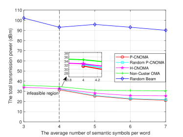

Fig. 8 and Fig. 9 illustrate the total transmission power as a function of the total transmission power versus the average number of semantic symbols per word () for different transmission schemes. The target semantic rate is set as 0.02 Msuts/s and 0.06 Msuts/s in Fig. 8 and Fig. 9, respectively. When 0.02 Msuts/s , an increase in leads to a general decrease in total transmission power across all schemes. This trend reflects the reduced power demand associated with higher density of semantic symbols. Although, the P-CNOMA scheme can achieve the lowest total transmission power, however, they encounter feasibility issues when the average number of semantic symbols per word is small. In this scenario, the H-CNOMA scheme effectively resolves the feasibility issue, albeit with a slightly higher transmission power consumption. When 0.06 Msuts/s , the total transmission power of the H-CNOMA scheme begins to increase again when exceeds 6. This occurs because the semantic rate is influenced by ; a larger reduces the semantic rate. Once surpasses 6, the semantic rate of the H-CNOMA scheme enters the semantic rate domination region. Consequently, the total transmission power rises as both the semantic rate and increase. The semantic rate of the non-cluster OMA scheme falls within the semantic rate domination region from the beginning, therefore, the total transmission power rises as increases. Moreover, this scheme has a significantly large infeasible region due to the introduction of additional frequency sub-channels, as indicated by (60).
Overall, both proposed MA transmission schemes effectively minimize total transmission power, but each is better suited to different scenarios. In particular, the P-CNOMA scheme offers a higher semantic rate as each user can utilize the entire bandwidth; however, this comes at the cost of restricting users’ demands. In contrast, the H-CNOMA scheme can accommodate any user demand when the semantic rate requirement remains below the maximum achievable semantic rate.
V Conclusion
This paper presents two innovative MA transmission schemes, the P-CNOMA scheme and the H-CNOMA scheme, designed to minimize total transmission power in a semantic-enhanced NOMA network. Both schemes effectively achieve low transmission power, but are suitable for different scenarios. The P-CNOMA scheme provides the lowest power consumption and higher semantic rates by allowing each user to utilize the full bandwidth. However, it is constrained by feasibility issues under high QoS demands due to inter-cluster interference. Conversely, the H-CNOMA scheme, while consuming slightly more power, is more adaptable, meeting diverse user requirements and managing interference effectively, especially when semantic rate demands fall below the maximum threshold. The results of this study offer valuable guidance for selecting appropriate MA schemes based on specific network conditions and user requirements. By highlighting the strengths and limitations of each approach, this work provides a framework for optimizing resource allocation in next-generation semantic communication networks, aiding in the design of power-efficient and adaptable wireless systems.
Appendix A Proof of Lemma 1
According to (6), is positive and represents the SNR, which is positive. Therefore, we have
The direction of an inequality is not affected when the same number is added to both sides. Hence, we have
Note , after the algebraic transformation, is proved.
Appendix B Proof of Proposition 1
Appendix C Proof of Proposition 2
The Lagrangian function of can be expressed as
| (62) |
where , , , , , , and are Lagrangian multipliers of inequality constraints and is the Lagrangian multiplier of the equality constraint. Let , , , , , , , and denote the optimal Lagrangian multiplier. According to the Karush-Kuhn-Tucker (KKT) conditions, the following inequalities hold, which can be formulated as
| (63) |
| (64) |
Without loss of generality, we take as an example to analyze the rank condition. Since is a convex problem, the KKT conditions should be satisfied. According to the stationarity and complementary slackness, we have
| (65) |
and
| (66) |
where denotes the identical matrix and denotes the matrix with all elements are 0. The dimension of and are aligned with the dimension of . According to (65),
| (67) |
where , can be obtained. Let represent the maximum eigenvalue of . Given the inherent randomness of channels, the probability that the channel-determined matrix has more than one same maximum eigenvalues is nearly zero, leading to the following discussions:
-
•
If , has a negative eigenvalue, which violates (64).
-
•
If , all eigenvalue are positive, which shows is a full rank matrix. According to (66), , which is not reasonable in practice.
-
•
If , and all other eigenvalues of are smaller than , hence, the rank of . According to (66), the rank of is 1.
As a result, . This proof is also applicable to other beamforming matrices. The proposition is proved.
Appendix D Proof of Proposition 3
Constraint (52b) can be rewritten as
| (68) |
There always exists a that satisfies (68) only when and is not orthogonal to .
Constraints (52c) and (52d) can be rewritten as
| (69) |
and
| (70) |
respectively. We notice that there always exists a that can satisfy (69) and (70) when and is not orthogonal to and .
As a result, if is feasible, the conditions that and is not orthogonal to and should be satisfied. The proposition is proved.
References
- [1] P. V. Matre, A. Kumbhare, R. Gedam, A. Sharma, N. K. Vaishnav, and D. Naidu, “6G enabled smart iot in healthcare system: Prospect, issues and study areas,” in 2023 International Conference on Artificial Intelligence for Innovations in Healthcare Industries (ICAIIHI), vol. 1. IEEE, 2023, pp. 1–6.
- [2] M.-H. Chen, K.-W. Hu, I.-H. Chung, and C.-F. Chou, “Towards VR/AR multimedia content multicast over wireless LAN,” in 2019 16th IEEE Annual Consumer Communications & Networking Conference (CCNC). IEEE, 2019, pp. 1–6.
- [3] Z. Ding, X. Lei, G. K. Karagiannidis, R. Schober, J. Yuan, and V. K. Bhargava, “A survey on non-orthogonal multiple access for 5G networks: Research challenges and future trends,” IEEE J. Sel. Areas Commun., vol. 35, no. 10, pp. 2181–2195, 2017.
- [4] F. Fang, K. Wang, Z. Ding, and V. C. Leung, “Energy-efficient resource allocation for NOMA-MEC networks with imperfect CSI,” IEEE Trans. Commun., vol. 69, no. 5, pp. 3436–3449, 2021.
- [5] W. Tong and G. Y. Li, “Nine challenges in artificial intelligence and wireless communications for 6G,” IEEE Wirel. Commun., vol. 29, no. 4, pp. 140–145, 2022.
- [6] W. Yang, H. Du, Z. Q. Liew, W. Y. B. Lim, Z. Xiong, D. Niyato, X. Chi, X. Shen, and C. Miao, “Semantic communications for future internet: Fundamentals, applications, and challenges,” IEEE Commun. Surv. Tutor., vol. 25, no. 1, pp. 213–250, 2022.
- [7] X. Luo, H.-H. Chen, and Q. Guo, “Semantic communications: Overview, open issues, and future research directions,” IEEE Wirel. Commun., vol. 29, no. 1, pp. 210–219, 2022.
- [8] W. Huang, J. Wang, X. Chen, Q. Peng, and Y. Zhu, “Flag vector assisted multi-user semantic communications for downlink text transmission,” IEEE Commun. Lett., 2024.
- [9] Z. Weng, Z. Qin, X. Tao, C. Pan, G. Liu, and G. Y. Li, “Deep learning enabled semantic communications with speech recognition and synthesis,” IEEE Trans. Wirel. Commun., vol. 22, no. 9, pp. 6227–6240, 2023.
- [10] C. Liang, D. Li, Z. Lin, and H. Cao, “Selection-based image generation for semantic communication systems,” IEEE Commun. Lett., 2023.
- [11] Z. Zhang, Q. Yang, S. He, and J. Chen, “Deep learning enabled semantic communication systems for video transmission,” in 2023 IEEE 98th Vehicular Technology Conference (VTC2023-Fall). IEEE, 2023, pp. 1–5.
- [12] C. E. Shannon and W. Weaver, The mathematical theory of communication. Champaign, IL: U. Illinois Press, 1949.
- [13] O. Lassila, J. Hendler, and T. Berners-Lee, “The semantic web,” Scientific American, vol. 284, no. 5, pp. 34–43, 2001.
- [14] J. Choi, S. W. Loke, and J. Park, “A unified view on semantic information and communication: A probabilistic logic approach,” in 2022 IEEE International Conference on Communications Workshops (ICC Workshops). IEEE, 2022, pp. 705–710.
- [15] H. Xie, Z. Qin, G. Y. Li, and B.-H. Juang, “Deep learning enabled semantic communication systems,” IEEE Trans. Signal Process., vol. 69, pp. 2663–2675, 2021.
- [16] H. Xie, Z. Qin, and G. Y. Li, “Task-oriented multi-user semantic communications for VQA,” IEEE Wireless Commun. Lett., vol. 11, no. 3, pp. 553–557, 2021.
- [17] Z. Lyu, G. Zhu, J. Xu, B. Ai, and S. Cui, “Semantic communications for image recovery and classification via deep joint source and channel coding,” IEEE Trans. Wirel. Commun., 2024.
- [18] W. Li, H. Liang, C. Dong, X. Xu, P. Zhang, and K. Liu, “Non-orthogonal multiple access enhanced multi-user semantic communication,” IEEE Trans. Cogn. Commun. Netw., 2023.
- [19] X. Mu and Y. Liu, “Exploiting semantic communication for non-orthogonal multiple access,” IEEE J. Sel. Areas Commun., 2023.
- [20] X. Mu, Y. Liu, L. Guo, and N. Al-Dhahir, “Heterogeneous semantic and bit communications: A semi-NOMA scheme,” IEEE J. Sel. Areas Commun., vol. 41, no. 1, pp. 155–169, 2023.
- [21] Z. Ding, L. Lv, F. Fang, O. A. Dobre, G. K. Karagiannidis, N. Al-Dhahir, R. Schober, and H. V. Poor, “A state-of-the-art survey on reconfigurable intelligent surface-assisted non-orthogonal multiple access networks,” Proc. IEEE., vol. 110, no. 9, pp. 1358–1379, 2022.
- [22] Z. Ding, P. Fan, and H. V. Poor, “Impact of user pairing on 5G nonorthogonal multiple-access downlink transmissions,” IEEE Trans. Veh. Technol., vol. 65, no. 8, pp. 6010–6023, 2015.
- [23] J. Guo, X. Wang, J. Yang, J. Zheng, and B. Zhao, “User pairing and power allocation for downlink non-orthogonal multiple access,” in 2016 IEEE Globecom Workshops (GC Wkshps). IEEE, 2016, pp. 1–6.
- [24] H. Xie, Z. Qin, G. Y. Li, and B.-H. Juang, “Deep learning enabled semantic communication systems,” IEEE Trans. Signal Process., vol. 69, pp. 2663–2675, 2021.
- [25] L. Yan, Z. Qin, R. Zhang, Y. Li, and G. Y. Li, “Resource allocation for text semantic communications,” IEEE Wireless Commun. Lett., vol. 11, no. 7, pp. 1394–1398, 2022.
- [26] Z. Luo, W. Ma, A. M. C. So, Y. Ye, and S. Zhang, “Semidefinite relaxation of quadratic optimization problems,” IEEE Signal Process. Mag., vol. 27, no. 3, pp. 20–34, 2010.