Possible scenario of dynamical chiral symmetry breaking in the interacting instanton liquid model
Abstract
We compute the vacuum energy density as a function of the quark condensate in the interacting instanton liquid model (IILM) and examine the pattern of dynamical chiral symmetry breaking from its behavior around the origin. This evaluation is performed by using simulation results of the IILM. We find that chiral symmetry is broken in the anomaly assisted way in the IILM with three-flavor dynamical quarks. We call such a symmetry breaking the anomaly-driven breaking which is one of the scenarios of chiral symmetry breaking proposed in the context of the chiral effective theories. We also find that the instanton-quark interaction included in the IILM plays a crucial role for the anomaly-driven breaking by comparing the full and the quenched IILM calculations.
I Introduction
In hadron physics, chiral symmetry and its dynamical breaking have led to our systematic understanding of hadron spectra. For instance, the arrangement of light pseudoscalar -mesons can be explained through the dynamical breaking of flavor symmetry as the Nambu-Goldstone theorem states. On the other hand, mesons like are still puzzles in hadron physics Pelaez:2016 ; PDG:2022 . The characteristics of , such as its existence, mass and internal structure, have been under discussion for a long time Jaffe:1977 ; Oller:1999 ; Black:1999 ; Ishida:1999 ; Colangelo:2001 ; Kunihiro:2004 ; Napsuciale:2004 ; Pelaez:2004 ; Mennessier:2011 ; Caprini:2006 ; Pennington:2007 ; Fariborz:2009 ; Hyodo:2010 ; Mennessier:2011 ; Parganlija:2013 ; Pelaez:2017 ; Ablikim:2019 ; Soni:2020 ; Achasov:2021 ; Pelaez:2021 . The meson that is recognized as the chiral partner of the pion is one of the candidates of because it should exist in the state if chiral symmetry is manifested in the low-energy regime of quantum chromodynamics (QCD). Since the meson emerges as a fluctuation of an order parameter of chiral symmetry, there is a growing need to systematically investigate the chiral dynamics.
In revealing such hadron properties, we need to understand the pattern of dynamical chiral symmetry breaking of QCD. Many models have been proposed to describe the dynamical chiral symmetry breaking GellMann:1960 ; Nambu:1961 ; Verbaarschot:2000 . A notable example is the Nambu-Jona-Lasinio (NJL) model which exhibits essential features of QCD and provides a mathematically traceable framework under the mean field approximation. In this model, the attractive interaction among quark fields induces the quark condensate in the vacuum and it breaks chiral symmetry. As chiral symmetry is broken dynamically, pseudoscalar mesons become the massless Nambu-Goldstone bosons, while their chiral partners, the scalar mesons, acquire finite masses. Furthermore, the inclusion of the anomaly enables us to comprehend the spectrum of pseudoscalar mesons including and Witten:1979 ; tHooft:1976_a ; tHooft:1976_b . Comprehensive understanding of the pattern and mechanism of dynamical chiral symmetry breaking is one of the keys to unraveling the properties of hadrons and the QCD vacuum on which they rely.
Recently, the chiral effective theories have shown that the different patterns of dynamical chiral symmetry breaking predict the different values of the mass Kono:2021 . In the NJL model without the anomaly term, chiral symmetry breaks dynamically when the interquark attractive interaction is sufficiently strong. With the presence of the anomaly term, chiral symmetry is broken dynamically even if the four-point interquark interaction is smaller than its critical value as long as the contribution from the anomaly is significant (which we call anomaly-driven symmetry breaking). The mass of the meson assumed as the chiral partner of the pion shows that in the former case it is larger than approximately , while in the latter case it is smaller than about Kono:2021 . These findings are derived from analyses using the linear sigma model and the NJL model, while the universality of their consequence remains unclear in other systems.
In this paper, we examine whether the anomaly-driven breaking of chiral symmetry universally realizes in the context of other than the chiral effective models. The realization of the anomaly-driven breaking is identified by the quark condensate dependence of the vacuum energy density. This characteristic is deduced from the discussion within the chiral effective models Kono:2021 . We generalize this concept to validate it in other models using the curvature of the vacuum energy density with respect to the quark condensate at the origin. As an example of its application, we use the interacting instanton liquid model (IILM). The IILM is a phenomenological model that describes the chiral symmetry breaking by treating the QCD vacuum as a superposition of instantons Shuryak:1982_1 ; Shuryak:1982_2 . Since the instanton results in the anomaly tHooft:1986 , we discuss the possibility of the anomaly-driven symmetry breaking using the IILM that has both features like the chiral symmetry breaking and the anomaly related to the instantons.
This paper is organized as follows. In Sect. II, we introduce the definition of anomaly-driven breaking of chiral symmetry in the NJL model and other models. In Sect. III, we describe the formulation of the IILM that is used in this study and details the numerical simulations. In Sect. IV, we present the simulation results of the IILM and discuss their interpretations. In Sect. V, we conclude this paper.
II Anomaly-driven breaking of chiral symmetry
In this section, we introduce the definition of the anomaly-driven chiral symmetry breaking in the NJL model and other models.
II.1 Anomaly-driven breaking in the NJL model
We briefly explain the anomaly-driven breaking of chiral symmetry which was proposed by the previous work Kono:2021 based on the three flavor NJL model with the axial anomaly term. In Ref. Kono:2021 , the following Lagrangian is considered:
| (1) | |||||
for the quark fields , where is the quark mass matrix given by with assuming isospin symmetry , represent the Gell-Mann matrices in the flavor space with , is understood as determinant operation over the flavor indices of the quark fields , and are the coupling constants for the four-point vertex interaction and the determinant-type breaking interaction, respectively. In the mean field approximation, the effective potential is obtained from the Lagrangian (1) as a function of the dynamical quark mass as follows
| (2) | |||||
where is the quark condensate with isospin symmetry and is given as a function of . Their specific forms are given by Eq. (A.1) and Eq. (A.2) in Ref. Kono:2021 .
Following Ref. Kono:2021 , we start with the case of the chiral limit and no anomaly term, i.e., and in Eq. (1). In this situation, chiral symmetry is dynamically broken at the vacuum with a finite dynamical quark mass when the dimensionless coupling constant is larger than . Here, is the critical coupling constant defined by with a three-momentum cutoff for the quark loop function. In other words, if there exists sufficiently strong four-quark interaction, chiral symmetry is dynamically broken in the vacuum. This is the well-known scenario of the dynamical chiral symmetry breaking in the NJL model.
Next, let us take the anomaly term into account with in Eq. (1) while keeping the chiral limit. In this situation, even though is less than , chiral symmetry can be broken dynamically in the vacuum due to the existence of the axial anomaly term. The previous work Kono:2021 demonstrated that such a situation is realized with a sufficiently large contribution from the anomaly term. We refer to such chiral symmetry breaking as the anomaly-driven breaking of chiral symmetry or shortly the anomaly-driven breaking in this paper.
The above patterns of the chiral symmetry breaking are related to the hadronic properties, such as the mass of the meson Kono:2021 . In the literature, in order to study the relationship more quantitatively, the explicit chiral symmetry breaking by finite current quark mass is introduced and the meson is assumed to be the chiral partner of the pion. The authors calculated the meson mass with varying values of the dimensionless couplings and so as to reproduce the mass. As a result, they found that the mass is smaller than about when the anomaly-driven breaking is realized, i.e., , and larger than about if the normal breaking is done, i.e., .
According to the previous work Kono:2021 , the definition of the anomaly-driven breaking in the NJL model is that the chiral symmetry is dynamically broken even though the dimensionless coupling constant is less than . However, the definition of this determination procedure relies on the model-specific parameter , which makes its application to other models nontrivial. To discuss the anomaly-driven breaking in other models and systems, in the next section, we generalize the definition of the determination procedure for the anomaly-driven breaking.
II.2 The anomaly-driven breaking in other models
In this subsection, we generalize the definition of the determination procedure for anomaly-driven breaking based on arguments in the NJL model. The anomaly-driven breaking of chiral symmetry was initially introduced in the chiral effective models using the model-specific coupling constants. Here, we present a key quantity that links the model-specific and the model-independent determination procedures for the anomaly-driven breaking. That is the sign of the curvature of the effective potential at the point with zero quark condensate. We use the latter as the definition of determination procedure for the anomaly-driven breaking in this paper.
We first consider the NJL model with no anomaly term in the vanishing quark mass limit . In this case, as we have mentioned in the last section, chiral symmetry is dynamically broken in the vacuum when a dimensionless four-quark coupling is greater than . Here, the evaluation of the second derivative of the effective potential (2) with respect to the quark condensate at the point yields the following result:
| (3) |
where we use . From Eq. (3), we find that the parameter region where chiral symmetry is dynamically broken is linked to the negativity of the curvature of the effective potential at the origin. We refer to such chiral symmetry breaking as the normal breaking in contrast to the anomaly-driven one.
Next, let us turn on the anomaly term by while keeping the chiral limit. Again, chiral symmetry can be dynamically broken and that leads to the nonzero quark condensate in the vacuum. The main difference compared to the case without the anomaly term is that chiral symmetry can be broken dynamically even though the dimensionless coupling is less than . Calculating the second derivative of the effective potential (2) with the anomaly term, we obtain the same result to Eq. (3). Thus, the pattern of dynamical chiral symmetry breaking which is distinguished whether is greater than or not corresponds directly to the sign of the curvature (3).
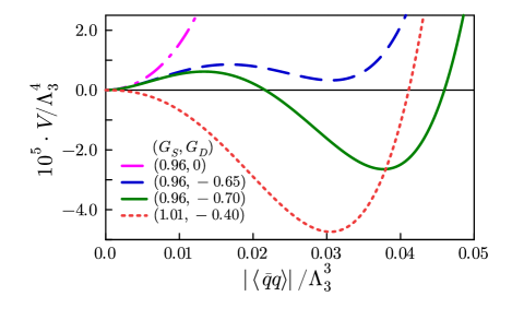
In Fig. 1, we show the effective potentials as a function of the absolute value of quark condensate for four parameter sets in the chiral limit. In order to set the origin to zero, irrelevant constants are subtracted from the effective potentials. We can see that when the dimensionless coupling is greater than , the curvature of effective potential at the origin is negative (red dotted line). On the other hand, when chiral symmetry is dynamically broken even though is less than (green solid line), the curvature is positive at the origin. For the remaining two parameter sets (magenta dash-dotted and blue dashed line), the effective potential has a minimum value at the origin and thus chiral symmetry is not broken in the vacuum. In this way, when the chiral symmetry is dynamically broken, the dimensionless coupling constant and the curvature of the effective potential at the origin are linked in the NJL model including the anomaly term for the chiral limit.
We also confirm that such a relationship between the dimensionless coupling and the curvature of the effective potential remains unchanged even if small current quark masses are introduced. The current quark mass dependence appears in the effective potential as a product with the linear term of the quark condensate for small quark masses. That term vanishes by performing the second derivative with respect to the quark condensate. Equation (3) thus remains the same in the presence of small current quark masses.
Based on the arguments in the NJL model, we use the curvature of the effective potential to determine whether the anomaly-driven breaking or not, instead of the model specific coupling constant. Since the effective potential is proportional to the vacuum energy density except for a constant in field theory, we take the inequality
| (4) |
to be the definition of the determination procedure for the anomaly-driven breaking also for finite quark masses. We apply this definition to the instanton liquid model and discuss the feasibility of the anomaly-driven chiral symmetry breaking.
III Formulation
In the present section, we describe the model and numerical calculation method we used.
III.1 Interacting instanton liquid model
The QCD Euclid partition function is approximated by the superposition of instantons Schafer:1996 . The canonical partition function is given as
| (5) | |||||
Here, and are the numbers of instantons and anti-instantons, respectively, is the measure of the path integral over the collective coordinate space for the color orientation in the color group, size and position associated with the -th instanton, and is semiclassical instanton amplitude. The interactions between instanton-instanton and instanton-quark are included in and , respectively. and represent the covariant derivative for the quark fields and the current quark mass of flavor , respectively.
The explicit expression of the semiclassical instanton amplitude calculated by ’t Hooft tHooft:1976_b reads
| (6) | |||||
| (7) |
where the gauge coupling is given as a function of the instanton size , the beta functions include up to 2-loop order and the Gell-Mann–Low coefficients are given as follows:
Here, and denote the number of colors and of the dynamical quark flavors, respectively, and is the scale parameter which is introduced for calculating -function by using the Pauli-Villars regularization scheme Schafer:1996 .
The instanton-instanton interaction in Eq. (5) is expressed by the sum of all possible pairs of instantons
| (10) |
where refer to each instanton or anti-instanton in the ensemble. The two-body interaction between instantons (or anti-instantons) is defined as the difference between the action of two-instanton configuration and twice of the single instanton action :
| (11) |
Two-instanton configuration is no longer an exact solution to the classical Yang-Mills equations. To calculate the two-body interaction, one uses an Ansatz for the gauge configurations. This idea was developed by Schäfer and Shuryak Schafer:1996 ; Schafer:1998 . We use the streamline Ansatz Yung:1988 ; Verbaarschot:1991 and its form of is given by Eq. (A5) in Ref. Schafer:1996 .
The instanton-quark interaction represented by the determinant in Eq. (5) is evaluated by factorizing it into two parts, a high and a low momentum parts as
| (12) |
The high momentum part is evaluated as the product of contributions of each instanton calculated by using the Gaussian approximation. The low momentum part is evaluated by using the quark zero-mode wave functions in the instanton and anti-instanton backgrounds Schafer:1996 . As a result, the instanton-quark interaction takes the following form:
| (13) | |||||
| (14) |
Here is called the overlap matrix with a size of . This matrix is spanned by the quark zero-mode wave functions in the instanton () and anti-instanton backgrounds which are labeled by the collective coordinate . The specific forms of the quark zero-mode wavefunctions are summarized in Appendix 2 of Ref. Schafer:1998 . The determinant operation is taken over the space represented in Eq. (13) and is understood as a diagonal matrix of . The explicit expression of is given by Eq. (B2) in Ref. Schafer:1996 .
In this paper, we work on the flavor symmetric limit, i.e., the number of quark flavors is set to and the current quark masses are equally set to . The quark condensate represents the one-flavor amount for our calculations.
III.2 Free energy in instanton ensemble
The vacuum energy density is identified the free energy density as at zero temperature and we simply call it the free energy denoted as in what follows. This relationship is derived from the standard thermodynamics relation. The free energy is expressed as
| (15) |
with the four-dimensional space-time volume and the partition function of the system considered.
We explain the method to compute the value of the partition function . The method that we use is well-known as the thermodynamics integration method, and it has been applied to the IILM calculation in the previous work Schafer:1996 . In this method, one writes the effective action as
| (16) |
with the partition function . The desired partition function is reproduced as . This form of the effective action (16) interpolates between a known solvable action and the full action . One obtains the partition function straightforwardly as
| (17) |
where the expectation value is defined by
| (18) |
with configurations according to . Therefore, if we know the decomposition (16) and the values of and , we can compute the partition function from Eq. (17).
For our computation of the partition function in the instanton liquid model, we use the following decomposition of the effective action as Ref. Schafer:1996 :
| (19) | |||||
where is a coefficient with the Gell-Mann–Low coefficient given by Eq. (III.1), and is the average size squared of instantons in the full ensembles including the instanton-instanton and instanton-quark interactions. The variational single instanton distribution is used as . Its form is given by
| (20) |
with
| (21) |
III.3 Quark condensate in instanton ensemble
In the instanton liquid model, the quark condensate is evaluated as the expectation value of the traced quark propagator at the same space-time coordinate as follows:
Here we write the measure of the path integral as in short that is given in the partition function (5), and represent the color and the Dirac indices, respectively and taken for the both indices. The quark propagator is approximated as a sum of contributions from the free and the zero-mode propagators by inverting the Dirac operator in the basis spanned by the quark zero-mode wave functions in instantons background as following Schafer:1998
where the matrix is the overlap matrix given in Eq. (13). Here we omit to write the collective coordinates of instantons from the argument of the quark zero-mode wave functions. We obtain the quark condensate by averaging it over the configurations.
III.4 Monte Carlo simulation
The simplest way to simulate the instanton liquid model described by the Euclid partition function (5) is to use the Monte Carlo method with a weight function given by
| (24) |
To perform Monte Carlo simulations using the Markov Chain Monte Carlo (MCMC) method, it is crucial to understand the weight function . This function represents the probability density as where denotes a configuration within the considered ensemble. Once the partition function is established, we derive the weight function, as illustrated in Eq. (24). Employing algorithms such as the Metropolis algorithm or Hybrid Monte Carlo (HMC) algorithm, we generate a series of configurations that converge to the given probability density function because of the detailed balance condition of the algorithms. Here, represents the number of configurations.
The expectation value of an operator that is expressed as a function of a configuration is computed from these configurations using the formula:
| (25) |
For more details on the Monte Carlo simulations using the MCMC, we referred to some textbooks and an introductory article Binder:2010 ; Randau:2014 ; Hanada:2018 .
IV Results
In this section, we will show our numerical results. In subsection IV.1, we explain the computational setup and numerical method used for our calculations. In subsection IV.2, we show our results of the free energy as a function of the instanton density. In subsection IV.3, we present the results of the quark condensate as a function of the instanton density. Combining these results, in subsection IV.4, we obtain the free energies as a function of the quark condensate and analyze them near the origin.
IV.1 Computational setup
In our simulations, each configuration consists of instantons and anti-instantons labeled by their collective coordinate and the partition function for each instanton density is determined by generating 5000 configurations after 1000 initial sweeps with instantons and anti-instantons. The simulations with different instanton density are achieved by changing the simulation box size with the fixed number of instantons . Whole simulations are performed under the periodic boundary condition for the coordinates of instantons and anti-instantons. All quantities in this calculation are nondimensionalized by which has been introduced through the -functions (III.1). The value of the scale parameter is determined so that the free energy has a minimum value at the instanton density Schafer:1996 . This density with the minimum free energy is the vacuum instanton density. We are interested in the quark condensate dependence of the free energy in the small quark mass regime, so we set the current quark masses to be as small as possible within a stable run of the simulations. The calculations below are performed with the current quark masses .
In Table 1, we show the bulk parameters, such as the current quark mass , the instanton density in the vacuum , the scale parameter and the instanton average size in our simulations. These values are consistent with the previous work Schafer:1996 . By fixing the unit such that at the vacuum, the values of the scale parameter are determined as for each current quark mass. Using these values, the average instanton sizes in our calculations are evaluated as to compared to in Ref. Schafer:1996 .
To calculate the free energy by Eq. (15), we need the value of the partition function. The partition function is obtained through Eq. (17), so we first calculate with the variational single instanton distribution (21). The single instanton distribution can be evaluated from initial 1000 sweeps with full interaction . We calculate the average size squared of instantons appearing in Eq. (21) using the initial sweeps. The -integral over an infinite interval appearing in Eq. (21) is practically performed over a finite interval . The remaining task for the calculation of the partition function is to perform the integral by summing the integrands. This integral is done at 10 different coupling values .
In the computation of the quark condensate, only the quark zero-mode propagator in Eq. (LABEL:eq:S_full) is evaluated to subtract the infinite contribution initiated by the free propagator at the same space-time coordinate. In the actual calculations, for each instanton density, the trace of the quark zero-mode propagator is averaged over the 5000 configurations, and also averaged over 10,000 different space-time coordinates to reduce the effect of incomplete equilibration of the configurations.
IV.2 Free energy
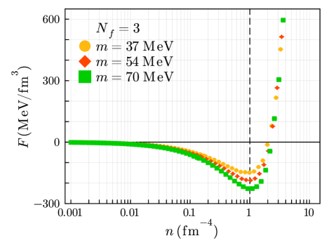
In Fig. 2, we show our numerical results of the free energies (in the unit of ) versus the instanton density (in the unit of ) for three values of the current quark mass. Our results are consistent with the previous work Schafer:1996 . The free energy is monotonically decreasing towards a minimum value and then rapidly increasing at higher instanton density. This shows that attractive interaction is dominant in lower instanton density regions, while repulsive interaction becomes important at higher instanton density.
In Table 2, we summarize our numerical results of the free energy and the quark condensate at the vacuum for three different current quark masses . By using the values of the scale parameter in Table 1, the free energies are evaluated as . For reference, we perform further calculations for the current quark masses with values close to those in the previous work, such as Schafer:1996 . That shows a good agreement with the previous work, and we conclude that our simulations work well.
IV.3 Quark condensate
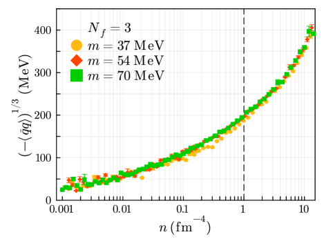
In Fig. 3, we show the instanton density dependence of cubic root of the quark condensate in the unit of . We find that the absolute values of the quark condensate increase monotonically as the instanton density increases. We also find that the value of the quark condensates at the vacuum is insensitive to the value of the current quark masses. This means that the contribution from the explicit breaking of chiral symmetry due to the current quark mass is not so large for the value of the quark condensate.
In Table 2, we show the values of the quark condensate at the vacuum instanton density. Our results almost reproduce the empirical values obtained by various previous works GellMann:1968 ; Reinders:1985 ; Dosch:1998 ; Harnett:2021 ; Giusti:2001 ; McNeile:2013 ; Borsanyi:2013 ; Durr:2014 ; Cossu:2016 ; Davies:2019 ; FLAG:2021 ; Gasser:1985 ; Jamin:2001 ; Boyle:2016 ; Kneur:2020 . We obtain the values of the quark condensate as at the vacuum with the current quark masses , respectively. These values give a good estimate of the quark condensates although they are slightly smaller in the absolute value.
IV.4 Free energy vs. quark condensate
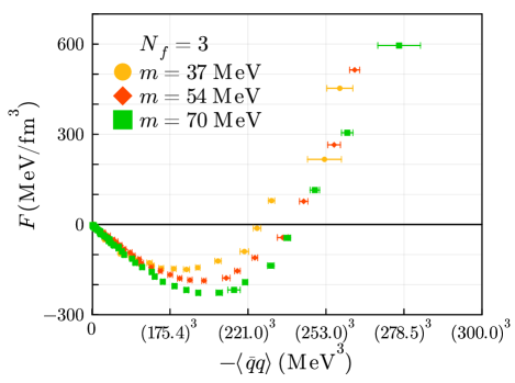
Combining the results of the free energy and the quark condensate, we obtain the quark condensate dependence of the free energy as shown in Fig. 4. The free energies monotonically decrease towards the minimum values as the quark condensate increases in magnitude. Once the free energies have the minimum value, they start to increase as expected from the instanton density dependence of them (also see Fig. 2). From this, we observe that the free energy has its minimum value at the point with the finite value of the quark condensate. This shows that chiral symmetry is dynamically broken in the vacuum of the IILM.
The behavior of the free energy near the origin appears to be decreasing in a downward convex trend. This trend is crucial for the sign of the curvature of the free energy at the origin. In other words, it provides one of the hints for discriminating patterns of chiral symmetry breaking through our definition of the determination procedure for the anomaly-driven breaking discussed in Sect. II.2. So we study the quark condensate dependence of the free energy more quantitatively.
We aim to evaluate the curvature of the free energy at the origin from our simulation results of the IILM. For that, we perform polynomial fits for our three data sets with different current quark masses. Each data set consists of pairs of and , i.e., arranged in ascending order, where is the number of data of the free energy and the quark condensate and it is equal to the number of the grid points of the instanton density, in our calculations.
We use a polynomial function given by
| (26) |
for the fitting model in this analysis. We perform the fits for four orders . For each order , we optimize the parameters so that they minimize the reduced chi-square including errors of both axes as given in Ref. Orear:1984 by
| (27) |
where with their errors correspond to our data set with their errors, and represent the fit model (26) and its first derivative, is the number of degrees of freedom which is defined by , and is the number of data used in the fit. We use the data from to rather all data because we want to know the behavior of the free energy around the origin.
We determine an upper limit of fit range, , as follows. We calculate the reduced chi-square (27) as we increase the number of data that we use and obtain the reduced chi-square as a function of the number of data. We then find the number of data for which the reduced chi-square has a local minimum value. We finally use this number of data as the value of for fitting. Here we skip a trivial local minimum obtained with a small number of data. The specific values of used in each fit, the corresponding quark condensate values and the reduced chi-square are summarized in Table 3.
| 37 | 54 | 70 | ||||
|---|---|---|---|---|---|---|
| 1 | ||||||
| 2 | ||||||
| 3 | ||||||
| 4 | ||||||
| 37 | 54 | 70 | ||||
|---|---|---|---|---|---|---|
| 1 | ||||||
| 2 | ||||||
| 3 | ||||||
| 4 | ||||||
In Table 4, we show the fit results of . We find that the value of the coefficient is close to zero. For different fit orders and quark masses, the values of range from to in the unit of . These values are sufficiently small compared to the typical value of the free energy and we conclude that the coefficient is consistent with zero.
| 37 | 54 | 70 | ||||
|---|---|---|---|---|---|---|
| 1 | ||||||
| 2 | ||||||
| 3 | ||||||
| 4 | ||||||
In Table 5, we show the fit results of . We find that the value of is insensitive to the fitting order . This implies that the value of is well determined around the origin. We find also that has no clear quark mass dependence. The averaged values of over the different orders are and for and .
| 37 | 54 | 70 | ||||
|---|---|---|---|---|---|---|
| 1 | - | - | - | |||
| 2 | ||||||
| 3 | ||||||
| 4 | ||||||
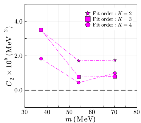
In Table 6, we show the fit results of . We find that the coefficients appear to be positive. For each quark mass, the averaged values of over the different fit orders are for and . These values of are located at the positive region for all orders and current quark masses. This suggests that the curvature of the free energy at the origin is positive for the IILM.
In Fig. 5, we show the current quark mass dependence of the coefficient . The value of is not very sensitive to the value of the current quark mass. For the fit with the smallest quark mass, the values of are evaluated as slightly larger than the results of other two quark masses. These results suggest that the value of and the curvature of the free energy at the origin is positive for wide current quark mass region and thus we conclude that the anomaly-driven breaking of chiral symmetry is realized in the IILM by our definition (4)
Here we do not show the values of the coefficients and because these coefficients are introduced to confirm the stability of fits of and with and without these higher-order terms. Furthermore, since we use the part of full data near the origin for fits, the values of and are not determined well and irrelevant to our discussion.
Interestingly we find the opposite sign of in the quenched calculations where the quark determinant part in the partition function (5) is set as in generating the configurations. The details of the quenched calculation are shown in Appendix A. As we show in Table 7, the quenched calculations suggest the negative values of coefficient . By our definition of the anomaly-driven breaking (4), this concludes that the normal breaking is realized in the quenched IILM. The opposite signs of obtained by the full and quenched calculations mean that the different scenarios of chiral symmetry breaking are possible depending on the presence of the quark determinant part in the IILM partition function. Since the quark determinant contributes to the instanton-quark interaction in the ensemble, this implies that the quarks play a crucial role in the anomaly-driven breaking for the IILM.
| Quenched | ||||||
| 2.8 | 14 | 28 | ||||
| 1 | - | - | - | |||
| 2 | ||||||
| 3 | ||||||
| 4 | ||||||
V Conclusions
We have examined the possibility of the chiral symmetry breaking scenario that can be realized when the anomaly contribution is sufficiently large using the IILM. Following the NJL model, we have generalized the determination procedure for the pattern of chiral symmetry breaking. We use the second-order differential coefficient of the vacuum energy density with respect to the quark condensate at the origin, e.g., the curvature. We have defined that the pattern of chiral symmetry breaking is the normal or the anomaly-driven one if the curvature is negative or positive, respectively.
We have found that the curvature appears to be positive in the IILM. This means that the anomaly-driven breaking is feasible in the IILM by our definition. In contrast to that, the quenched calculations show the negative curvature and support the realization of the normal chiral symmetry breaking in the quenched IILM. These results indicate that the instanton-quark interaction is crucial to realize the anomaly-driven breaking because the difference between the full and quenched IILM is the presence or absence of the quark determinant that contributes to the interaction among instantons and the dynamical quarks.
One important direction for future development is to investigate the mass of mesons, such as and . As discussed in the previous work Kono:2021 , chiral effective theories concluded that the mass could be smaller than in the anomaly-driven symmetry breaking. We expect the same conclusions to be drawn in the IILM. Even if such conclusions cannot be reached, it is interesting to clarify the differences between the chiral effective theories and the IILM. Computation with different flavors, e.g., , using the IILM may provide further insights into the anomaly-driven breaking in QCD. These are subjects to be investigated in future studies.
Acknowledgments
We would like to thank Masayasu Harada for useful discussions and comments. We also thank Masakiyo Kitazawa and Kotaro Murakami for their advice. This work of Y.S. was partly supported by the Advanced Research Center for Quantum Physics and Nanoscience, Tokyo Institute of Technology, and JST SPRING, Grant Number JPMJSP2106. The work of D.J. was supported in part by Grants-in-Aid for Scientific Research from JSPS (JP21K03530, JP22H04917 and JP23K03427).
Appendix A Results of the quenched calculations
We show the numerical results for the quenched calculations. The quenched calculations can be performed in the same way as in the full calculations except for setting the quark determinant in the partition function to unity. The following numerical results of the quenched calculations are obtained by the same setup as the full calculations, that is, 5000 configurations after 1000 initial sweeps with instantons and anti-instantons. In the quenched calculations, the current quark mass enters only the calculation of the quark condensate through the quark zero-mode propagator (LABEL:eq:S_full).
In Table 8, we show the bulk parameters of the quenched ensemble. These values are consistent with the quenched calculation in the previous work Schafer:1996 . We obtain the scale parameter and the average instanton size , which are compared to and in the previous work Schafer:1996 , respectively. Our result of the free energy shows a good agreement with for the quenched calculation in Ref. Schafer:1996 . Our result also shows a good agreement with the estimation from the trace anomaly as discussed in Ref. Schafer:1996 .
| Quenched | |||
|---|---|---|---|
In Table 9, we show the quark condensate at the vacuum for three current quark masses. Our results of the quark condensate for the current quark masses almost reproduce the empirical values obtained by various previous works GellMann:1968 ; Reinders:1985 ; Dosch:1998 ; Harnett:2021 ; Giusti:2001 ; McNeile:2013 ; Borsanyi:2013 ; Durr:2014 ; Cossu:2016 ; Davies:2019 ; FLAG:2021 ; Gasser:1985 ; Jamin:2001 ; Boyle:2016 ; Kneur:2020 . We conclude that our simulations also work well in the quenched calculations.
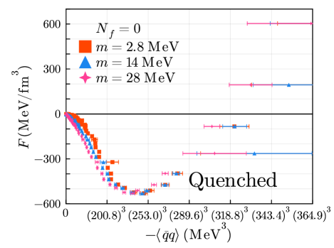
In Fig. 6, we show the free energy versus the quark condensate for the quenched calculations. This shows globally almost same behavior with the results of the unquenched calculations, but the trend of the free energy near the origin appears to be slightly different from the unquenched results. We perform the same analysis to the unquenched calculations using the polynomial fitting and show the fit results following.
| Quenched | ||||||
|---|---|---|---|---|---|---|
| 2.81 | 14.04 | 28.08 | ||||
| 1 | ||||||
| 2 | ||||||
| 3 | ||||||
| 4 | ||||||
| Quenched | ||||||
|---|---|---|---|---|---|---|
| 2.81 | 14.04 | 28.08 | ||||
| 1 | ||||||
| 2 | ||||||
| 3 | ||||||
| 4 | ||||||
In Table 10, we show the fit results of for the quenched calculations. We find that the value of the coefficient is also close to zero. The value of averaged over different orders and quark masses is . This value is sufficiently small compared to the typical value of the free energy and we conclude that the coefficient is also consistent with zero in the quenched calculation.
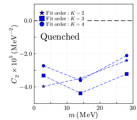
In Table 11, we show the fit results of for the quenched calculations. We find that the coefficient increases monotonically as the current quark mass increases. For each quark mass, we average the values of over the different orders and obtain , and for and , respectively. We conclude that the value of increases monotonically as the quark mass increases for the quenched calculations.
In Fig. 7, we show the current quark mass dependence of the coefficient for the quenched calculations. For all quark masses, the value of appears to be negative in different fit orders. As we have discussed in Sect. IV.4, these results suggest that the chiral symmetry is broken in the normal way for the quenched IILM by our definition (4).
References
- (1) J. R. Peláez, “From controversy to precision on the sigma meson: A review on the status of the non-ordinary resonance,” Phys. Rept. 658 (2016) 1.
- (2) R. L. Workman, et al., (Particle Data Group), “Review of Particle Physics,” Prog. Theor. Exp. Phys. 2022, 083C01 (2022).
- (3) R. J. Jaffe, “Multiquark hadrons. I. Phenomenology of mesons,” Phys. Rev. D 15 (1977) 267.
- (4) J. A. Oller, E. Oset, “Meson-meson interactions in a nonperturbative chiral approach,” Phys. Rev. D 59 (1999) 074001; Erratum: [Phys. Rev. D 60 (1999) 099906, Phys. Rev. D 75 (2007) 099903].
- (5) D. Black, A. H. Fariborz, F. Sannino, J. Schechter, “Putative light scalar nonet,” Phys. Rev. D 59 (1999) 074026.
- (6) M. Ishida, “Possible Classification of the Chiral Scalar -Nonet,” Prog. Theor. Phys. 101 (1999) 661.
- (7) G. Colangelo, J. Gasser, H. Leutwyler, “ scattering,” Nucl. Phys. B 603 (2001) 125.
- (8) T. Kunihiro, S. Muroya, A. Nakamura, C. Nonaka, M. Sekiguchi, H. Wada, “Scalar mesons in lattice QCD,” Phys. Rev. D 70 (2004) 034504.
- (9) M. Napsuciale, S. Rodriguez, “Chiral model for and mesons,” Phy. Rev. D 70 (2004) 094043.
- (10) J. R. Peláez, “Light scalars as tetraquarks or two-meson states from large- and unitarized chiral perturbation theory,” Mod. Phys. Lett. A 39 (2004) 2879.
- (11) I. Caprini, G. Colangelo, H. Leutwyler, “Mass and Width of the Lowest Resonance in QCD,” Phys. Rev. Lett. 96 (2006) 132001.
- (12) M. R. Pennington, “Location, correlation, radiation: Where is the , what is its structure, and what is its coupling to photons?,” Mod. Phys. Lett. A 22 (2007) 1439.
- (13) A. H. Fariborz, R. Jora, J. Schechter, “Global aspects of the scalar meson puzzle,” Phys. Rev. D 79 (2009) 074014.
- (14) T. Hyodo, D. Jido, T. Kunihiro, “Nature of the meson as revealed by its softening process,” Nucl. Phys. A 848 (2010) 341.
- (15) G. Mennessier, S. Narison, X.-G. Wang, “ and substructures from radiative and semi-leptonic decays,” Phy. Lett. B 696 (2004) 40.
- (16) D. Parganlija, P. Kovács, Gy. Wolf, F. Giacosa, D. H. Rischke, “Meson vacuum phenomenology in a three-flavor linear sigma model with (axial-)vector mesons,” Phys. Rev. D 87 (2013) 014011.
- (17) J. R. Peláez, A. Rodas, J. Ruiz de Elvira, “Strange resonance poles from scattering below 1.8 GeV,” Eur. Phys. J. C 77 (2017) 91.
- (18) M. Ablikim, et al. (BESIII Collaboration), “Observation of and Improved Measurements of ,” Phys. Rev. Lett. 122 (2019) 062001.
- (19) N. R. Soni, A. N. Gadaria, J. J. Patel, J. N. Pandya, “Semileptonic decays of charmed mesons to light scalar mesons,” Phys. Rev. D 102 (2020) 016013.
- (20) N. N. Achasov, J. V. Bennett, A. V. Kiselev, E. A. Kozyrev, G. N. Shestakov, “Evidence of the four-quark nature of and ,” Phys. Rev. D 103 (2021) 014010.
- (21) J. R. Peláez, A. Rodas, J. Ruiz de Elvira, “Precision dispersive approaches versus unitarized chiral perturbation theory for the lightest scalar resonances and ,” Eur. Phy. J. Spec. Top. 230 (2021) 1539.
- (22) M. Gell-Mann, M. Lévy, “The Axial Vector Current in Bet Decay,” Nuovo. Cim. 16 (1960) 705.
- (23) Y. Nambu, G. Jona-Lasinio, “Dynamical Model of Elementary Particles Based on an Analogy with Superconductivity. I,” Phys. Rev. 112 (1961) 345.
- (24) J. J. M. Verbaarschot, T. Wettig, “Random matrix theory and chiral symmetry in QCD,” Ann. Rev. Nucl. Part. Sci. 50 (2000) 343.
- (25) E. Witten, “Current algebra theorem for the ”Goldstone Boson”,” Nucl. Phys. B 156 (1979) 269.
- (26) G. ’t Hooft, “Symmetry breaking through Bell–Jackiw anomalies,” Phys. Rev. Lett. 37 (1976) 8.
- (27) G. ’t Hooft, “Computation of the quantum effects due to four-dimensional pseudoparticle,” Phys. Rev. D 14 (1976) 3432.
- (28) S. Kono, D. Jido, Y. Kuroda, and M. Harada, “The role of UA(1) breaking term in dynamical chiral symmetry breaking of chiral effective theories,” PTEP 2021, no. 9, 093D02 (2021).
- (29) E. V. Shuryak, “The role of instantons in quantum chromodynamics: (I). Physical vacuum,” Nucl. Phys. B 203 (1982) 93.
- (30) E. V. Shuryak, “The role of instantons in quantum chromodynamics: (II). Hadronic structure,” Nucl. Phys. B 203 (1982) 116.
- (31) G. ’t Hooft, “How Instantons Solve the U(1) Problem,” Phys. Rept. 142, 357 (1986).
- (32) T. Scháfer and E. V. Shuryak, “Instantons in QCD,” Rev. Mod. Phys. 70 (1998) 323.
- (33) T. Scháfer and E. V. Shuryak, “Interacting instanton liquid model in QCD at zero and finite temperature,” Phys. Rev. D 53 (1996) 6522.
- (34) A. V. Yung, “Instanton vacuum in supersymmetric QCD,” Nucl. Phys. B 297 (1988) 47.
- (35) J. J. M. Verbaarschot, “Streamlines and conformal invariance in Yang-Mills theories,” Nucl. Phys. B 362 (1991) 33.
- (36) K. Binder and D. Herrmann, “Monte Carlo Simulations in Statistical Physics An Introduction (6th ed.),” Springer Berlin, Heidelberg (2010).
- (37) D. Randau and K Binder, “A Guide to Monte Carlo Simulations in Statistical Physics,” Cambridge Univ. Press. (2014).
- (38) M. Hanada, “Markov Chain Monte Carlo for Dummies,” arXiv:1808.08490.
- (39) M.A. Shifman, A.I. Vainshtein, V.I. Zakharov, “QCD and resonance physics. Applications,” Nucl. Phys. B 147 (1979) 448.
- (40) M. Gell-Mann, R.J. Oakes, B. Renner, “Behavior of current divergences under ,” Phys. Rev. 175 (1968) 2195.
- (41) L.J. Reinders, H. Rubinstein, S. Yazaki, “Hadron properties from QCD sum rules,” Phys. Rep. 127 (1985) 1.
- (42) H.G. Dosch, S. Narison, “Direct extraction of the chiral quark condensate and bounds on the light quark masses,” Phys. Lett. B 417 (1998) 173.
- (43) D. Harnett, J. Ho, T.G. Steele, “Correlations between the strange quark condensate, strange quark mass, and kaon PCAC relation,” Phys. Rev. D 103 (2021) 114005.
- (44) L. Giusti, C. Hoelbling, C. Rebbi, “Light quark masses with overlap fermions in quenched QCD,” Phys. Rev. D 64 (2001) 114508.
- (45) C. McNeile, A. Bazavov, C.T.H. Davies, R.J. Dowdall, K. Hornbostel, G.P. Lepage, H.D. Trottier, “Direct determination of the strange and light quark condensate from full lattice QCD,” Phys. Rev. D 87 (2013) 034503.
- (46) S. Borsányi, S. Dürr, Z. Fodor, S. Krieg, A. Schäfer, E.E. Scholz, K.K. Szabó, “SU(2) chiral perturbation theory low-energy constants from flavor staggered lattice simulations,” Phys. Rev. D 88 (2013) 014513.
- (47) S. Dürr, Z. Fodor, C. Hoelbling, S. Krieg, T. Kurth, L. Lellouch, T. Lippert, R. Malak, T. Métivet, A. Portelli, A. Sastre, K.K. Szabó, “Lattice QCD at physical point meets chiral perturbation theory,” Phys. Rev. D 90 (2014) 114504.
- (48) G. Cossu, H. Fukaya, S. Hashimoto, T. Kaneko, J. Noaki, “Stochastic calculation of the Dirac spectrum on the lattice and a determination of chiral condensate in -flavor QCD,” PTEP 2016 (2016) 093B06.
- (49) C.T.H. Davies, K. Hornbostel, J.Komijani, J. Koponen, G.P. Lepage, A.T. Lytle, C. McNeile, HPQCD collaboration, “Determination of the quark condensate from heavy-light current-current correlators in full lattice QCD,” Phys. Rev. D 100 (2019) 034506.
- (50) FLAG collaborations, “FLAG Review 2021,” Eur. Phys. J. C (2022) 82:869.
- (51) J. Gasser, H. Leutwyler, “Chiral perturbation theory: expansions in the mass of the strange quark,” Nucl. Phys. B 250 (1985) 465.
- (52) M. Jamin, “Flavour-symmetry breaking of the quark condensate and chiral corrections to the Gell-Mann–Oakes–Renner relation,” Phys. Lett. B 538 (2001) 71.
- (53) P.A. Boyle, N.H. Christ, N. Garron, C. Jung, A. Jüttner, C. Kelly, R.D. Mawhinney, G. McGlynn, D.J. Murphy, S. Ohta, A. Portelli, C.T. Sachrajda, “Low energy constants of partially quenched chiral perturbation theory from domain wall QCD,” Phys. Rev. D 93 (2016) 054502.
- (54) J. Kneur, A. Neveu, “Chiral condensate and spectral density at full five-loop and partial six-loop orders of renormalization group optimized perturbation theory,” Phys. Rev. D 101 (2020) 074009.
- (55) J. Orear, “Least squares when both variables have uncertainties,” Am. J. Phys. 50 (1982) 912, Erratum: [Am. J. Phys. 52 (1984) 278].