Position Heaps for Cartesian-tree Matching
on Strings and Tries
Abstract
The Cartesian-tree pattern matching is a recently introduced scheme of pattern matching that detects fragments in a sequential data stream which have a similar structure as a query pattern. Formally, Cartesian-tree pattern matching seeks all substrings of the text string such that the Cartesian tree of and that of a query pattern coincide. In this paper, we present a new indexing structure for this problem, called the Cartesian-tree Position Heap (CPH). Let be the length of the input text string , the length of a query pattern , and the alphabet size. We show that the CPH of , denoted , supports pattern matching queries in time with space, where is the height of the CPH and is the number of pattern occurrences. We show how to build in time with working space. Further, we extend the problem to the case where the text is a labeled tree (i.e. a trie). Given a trie with nodes, we show that the CPH of , denoted , supports pattern matching queries on the trie in time with space. We also show a construction algorithm for running in time and working space.
1 Introduction
If the Cartesian trees and of two strings and are equal, then we say that and Cartesian-tree match (ct-match). The Cartesian-tree pattern matching problem (ct-matching problem) [18] is, given a text string and a pattern , to find all substrings of that ct-match with .
String equivalence with ct-matching belongs to the class of substring-consistent equivalence relation (SCER) [17], namely, the following holds: If two strings and ct-match, then and also ct-match for any . Among other types of SCERs ([3, 4, 5, 14, 15]), ct-matching is the most related to order-peserving matching (op-matching) [16, 7, 9]. Two strings and are said to op-match if the relative order of the characters in and the relative order of the characters in are the same. It is known that with ct-matching one can detect some interesting occurrences of a pattern that cannot be captured with op-matching. More precisely, if two strings and op-match, then and also ct-match. However, the reverse is not true. With this property in hand, ct-matching is motivated for analysis of time series such as stock charts [18, 11].
This paper deals with the indexing version of the ct-matching problem. Park et al. [18] proposed the Cartesian suffix tree (CST) for a text string that can be built in worst-case time or expected time, where is the length of the text string . The factor in the worst-case complexity is due to the fact that the parent-encoding, a key concept for ct-matching introduced in [18], is a sequence of integers in range . While it is not explicitly stated in Park et al.’s paper [18], our simple analysis (c.f. Lemma 9 in Section 5) reveals that the CST supports pattern matching queries in time, where is the pattern length and is the number of pattern occurrences.
In this paper, we present a new indexing structure for this problem, called the Cartesian-tree Position Heap (CPH). We show that the CPH of , which occupies space, can be built in time with working space and supports pattern matching queries in time, where is the height of the CPH. Compared to the afore-mentioned CST, our CPH is the first index for ct-matching that can be built in worst-case linear time for constant-size alphabets, while pattern matching queries with our CPH can be slower than with the CST when is large.
We then consider the case where the text is a labeled tree (i.e. a trie). Given a trie with nodes, we show that the CPH of , which occupies space, can be built in time and working space. We also show how to support pattern matching queries in time in the trie case. To our knowledge, our CPH is the first indexing structure for ct-matching on tries that uses linear space for constant-size alphabets.
Conceptually, our CPH is most related to the parameterized position heap (PPH) for a string [12] and for a trie [13], in that our CPHs and the PPHs are both constructed in an incremental manner where the suffixes of an input string and the suffixes of an input trie are processed in increasing order of their lengths. However, some new techniques are required in the construction of our CPH due to different nature of the parent encoding [18] of strings for ct-matching, from the previous encoding [3] of strings for parameterized matching.
2 Preliminaries
2.1 Strings and (Reversed) Tries
Let be an ordered alphabet of size . An element of is called a character. An element of is called a string. For a string , let denote the number of distinct characters in .
The empty string is a string of length 0, namely, . For a string , , and are called a prefix, substring, and suffix of , respectively. The set of prefixes of a string is denoted by . The -th character of a string is denoted by for , and the substring of a string that begins at position and ends at position is denoted by for . For convenience, let if . Also, let for any .
A trie is a rooted tree that represents a set of strings, where each edge is labeled with a character from and the labels of the out-going edges of each node is mutually distinct. Tries are natural generalizations to strings in that tries can have branches while strings are sequences without branches.
Let be any node of a given trie , and let denote the root of . Let denote the depth of . When , let denote the parent of . For any , let denote the -th ancestor of , namely, and for . It is known that after a linear-time processing on , for any query node and integer can be answered in time [6].
For the sake of convenience, in the case where our input is a trie , then we consider its reversed trie where the path labels are read in the leaf-to-root direction. On the other hand, the trie-based data structures (namely position heaps) we build for input strings and reversed tries are usual tries where the path labels are read in the root-to-leaf direction.
For each (reversed) path in such that with , let denote the string obtained by concatenating the labels of the edges from to . For any node of , let .
Let be the number of nodes in . We associate a unique id to each node of . Here we use a bottom-up level-order traversal rank as the id of each node in , and we sometimes identify each node with its id. For each node id () let , i.e., is the path string from node to the root .
2.2 Cartesian-tree Pattern Matching
The Cartesian tree of a string , denoted , is the rooted tree with nodes which is recursively defined as follows:
-
•
If , then is the empty tree.
-
•
If , then is the tree whose root stores the left-most minimum value in , namely, iff for any and for any . The left-child of is and the right-child of is .
The parent distance encoding of a string of length , denoted , is a sequence of integers over such that
Namely, represents the distance to from position to its nearest left-neighbor position that stores a value that is less than or equal to .
A tight connection between and is known:
Lemma 1 ([19]).
For any two strings and of equal length, iff .
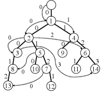
For two strings and , we write iff (or equivalently ). We also say that and ct-match when . See Fig. 1 for a concrete example.


We consider the indexing problems for Cartesian-tree pattern matching on a text string and a text trie, which are respectively defined as follows:
Problem 1 (Cartesian-Tree Pattern Matching on Text String).
- Preprocess:
-
A text string of length .
- Query:
-
A pattern string of length .
- Report:
-
All text positions such that .
Problem 2 (Cartesian-Tree Pattern Matching on Text Trie).
- Preprocess:
-
A text trie with nodes.
- Query:
-
A pattern string of length .
- Report:
-
All trie nodes such that .
2.3 Sequence Hash Trees
Let be a sequence of non-empty strings such that for any , for any . The sequence hash tree [8] of a sequence of strings, denoted , is a trie structure that is incrementally built as follows:
-
1.
for the empty sequence is the tree only with the root.
-
2.
For , is obtained by inserting the shortest prefix of that does not exist in . This is done by finding the longest prefix of that exists in , and adding the new edge , where is the first character of that could not be traversed in .
Since we have assumed that each in is not a prefix of for any , the new edge is always created for each . This means that contains exactly nodes (including the root).
To perform pattern matching queries efficiently, each node of is augmented with the maximal reach pointer. For each , let be the newest node in , namely, is the shortest prefix of which did not exist in . Then, in the complete sequence hash tree , we set iff is the deepest node in such that is a prefix of . Intuitively, represents the last visited node when we traverse from the root of the complete . Note that always holds. When (i.e. when the maximal reach pointer is a self-loop), then we can omit it because it is not used in the pattern matching algorithm.
3 Cartesian-tree Position Heaps for Strings

In this section, we introduce our new indexing structure for Problem 1. For a given text string of length , let denote the sequence of the parent distance encodings of the non-empty suffixes of which are sorted in increasing order of their lengths. Namely, , …, , …, , where . The Cartesian-tree Position Heap (CPH) of string , denoted , is the sequence hash tree of , that is, . Note that for each , holds.
Our algorithm builds for decreasing , which means that we process the given text string in a right-to-left online manner, by prepending the new character to the current suffix .
For a sequence of integers, let denote the sorted list of positions in such that iff . Clearly is equal to the number of ’s in .
Lemma 2.
For any string , .
Proof.
Let . We have that since otherwise for some , a contradiction. Thus holds. ∎
Lemma 3.
For each , can be computed from in an online manner, using a total of time with working space.
Proof.
Given a new character , we check each position in the list in increasing order. Let , i.e., is the global position in corresponding to in . If , then we set and remove from the list. Remark that these removed positions correspond to the front pointers in the next suffix . We stop when we encounter the first in the list such that . Finally we add the position to the head of the remaining positions in the list. This gives us for the next suffix .
It is clear that once a position in the PD encoding is assigned a non-zero value, then the value never changes whatever characters we prepend to the string. Therefore, we can compute from in a total of time for every . The working space is due to Lemma 2. ∎
A position in a sequence of non-negative integers is said to be a front pointer in if and . Let denote the sorted list of front pointers in . For example, if , then . The positions of the suffix which are removed from correspond to the front pointers in for the next suffix .
Our construction algorithm updates to by inserting a new node for the next suffix , processing the given string in a right-to-left online manner. Here the task is to efficiently locate the parent of the new node in the current CPH at each iteration.
As in the previous work on right-to-left online construction of indexing structures for other types of pattern matching [20, 10, 12, 13], we use the reversed suffix links in our construction algorithm for . For ease of explanation, we first introduce the notion of the suffix links. Let be any non-root node of . We identify with the path label from the root of to , so that is a PD encoding of some substring of . We define the suffix link of , denoted , such that iff is obtained by (1) removing the first (), and (2) substituting for the character at every front pointer of . The reversed suffix link of with non-negative integer label , denoted , is defined such that iff and . See also Figure 2.
Lemma 4.
Let be any nodes of such that with label . Then .
Proof.
Since , using Lemma 2, we obtain , where is a substring of such that . ∎∎
The next lemma shows that the number of out-going reversed suffix links of each node is bounded by the alphabet size.

Our CPH construction algorithm makes use of the following monotonicity of the labels of reversed suffix links:
Lemma 5.
Suppose that there exist two reversed suffix links and such that and . Then, .
Proof.
Immediately follows from , , and . ∎
We are ready to design our right-to-left online construction algorithm for the CPH of a given string . Since is the -th string of the input sequence , for ease of explanation, we will use the convention that and , where the new node for is inserted as a child of . See Figure 3.
Algorithm 1: Right-to-Left Online Construction of
- (base case):
-
We begin with which consists of the root and the node for the first (i.e. shortest) suffix of . Since , the edge from to is labeled . Also, we set the reversed suffix link .
- (iteration):
-
Given which consists of the nodes , which respectively represent some prefixes of the already processed strings , together with their reversed suffix links. We find the parent of the new node for , as follows: We start from the last-created node for the previous , and climb up the path towards the root . Let be the smallest integer such that the -th ancestor of has the reversed suffix link with the label . We traverse the reversed suffix link from and let . We then insert the new node as the new child of , with the edge labeled . Finally, we create a new reversed suffix link , where and . We set if the position is a front pointer of , and otherwise.
For computing the label efficiently, we introduce a new encoding that is defined as follows: For any string of length , let . The encoding preserves the ct-matching equivalence:
Lemma 6.
For any two strings and , iff .
Proof.
For a string , consider the DAG such that , (see also Figure 7 in Appendix). By Lemma 1, for any strings and , iff . Now, we will show there is a one-to-one correspondence between the DAG and the encoding.
() We are given for some (unknown) string . Since is the in-degree of the node of , is unique for the given DAG .
() Given for some (unknown) string , we show an algorithm that builds DAG . We first create nodes without edges, where all nodes in are initially unmarked. For each in decreasing order, if , then select the leftmost unmarked nodes in the range , and create an edge from each selected node to . We mark all these nodes at the end of this step, and proceed to the next node . The resulting DAG is clearly unique for a given . ∎
For computing the label of the reversed suffix link in Algorithm 1, it is sufficient to maintain the induced graph of DAG for a variable-length sliding window with the nodes . This can easily be maintained in total time.
Theorem 1.
Algorithm 1 builds for decreasing in a total of time and space, where is the alphabet size.
Proof.
Correctness: Consider the -th step in which we process . By Lemma 5, the -th ancestor of can be found by simply walking up the path from the start node . Note that there always exists such ancestor of since the root has the defined reversed suffix link . By the definition of and its reversed suffix link, is the longest prefix of that is represented by (see also Figure 3). Thus, is the parent of the new node for . The correctness of the new reversed suffix link follows from the definition.
Complexity: The time complexity is proportional to the total number of nodes that we visit for all . Clearly . Thus, . Using Lemma LABEL:lem:rsl_bounds and sliding-window , we can find the reversed suffix links in time at each of the visited nodes. Thus the total time complexity is . Since the number of nodes in is and the number of reversed suffix links is , the total space complexity is . ∎
Lemma 7.
There exists a string of length over a binary alphabet such a node in has out-going edges.
Proof.
Consider string . Then, for any , there exist nodes representing (see also Figure 6 in Appendix). Since , the parent node has out-going edges. ∎
Due to Lemma 7, if we maintain a sorted list of out-going edges for each node during our online construction of , it would require time even for a constant-size alphabet. Still, after has been constructed, we can sort all the edges offline, as follows:
Theorem 2.
For any string over an integer alphabet of size , the edge-sorted together with the maximal reach pointers can be computed in time and space.
Proof.
We sort the edges of as follows: Let be the id of each node . Then sort the pairs of the ids and the edge labels. Since and , we can sort these pairs in time by a radix sort. The maximal reach pointers can be computed in time using the reversed suffix links, in a similar way to the position heaps for exact matching [10]. ∎
See Figure 5 in Appendix for an example of with maximal reach pointers.
4 Cartesian-tree Position Heaps for Tries
Let be the input text trie with nodes. A naïve extension of our CPH to a trie would be to build the CPH for the sequence of the parent encodings of all the path strings of towards the root . However, this does not seem to work because the parent encodings are not consistent for suffixes. For instance, consider two strings and . Their longest common suffix is represented by a single path in a trie . However, the longest common suffix of and is . Thus, in the worst case, we would have to consider all the path strings , …, in separately, but the total length of these path strings in is .
To overcome this difficulty, we reuse the encoding from Section 3. Since is determined merely by the suffix , the encoding is suffix-consistent. For an input trie , let the FP-trie be the reversed trie storing for all the original path strings towards the root. Let be the number of nodes in . Since is suffix-consistent, always holds. Namely, is a linear-size representation of the equivalence relation of the nodes of w.r.t. . Each node of stores the equivalence class of the nodes in that correspond to . We set to be the representative of , as well as the id of node . See Figure 8 in Appendix.
Let be the set of distinct characters (i.e. edge labels) in and let . The FP-trie can be computed in time and working space by a standard traversal on , where we store at most front pointers in each node of the current path in due to Lemma 3.
Let be the node id’s of which are sorted in decreasing order. The Cartesian-tree position heap for the input trie is , where .
As in the case of string inputs in Section 3, we insert the shortest prefix of that does not exist in . To perform this insert operation, we use the following data structure for a random-access query on the PD encoding of any path string in :
Lemma 8.
There is a data structure of size
that can answer the following queries in time each.
Query input: The id of a node in and integer .
Query output: The th (last) symbol in .
Proof.
Let be the node with id , and . Namely, . For each character , let denote the nearest ancestor of such that the edge is labeled . If such an ancestor does not exist, then we set to the root .
Let , and be the label of the edge . Let be an empty set. For each character , we query . If and , then is a candidate for and add to set . After testing all , we have that . See Figure 4.

For all characters and all nodes in , can be pre-computed in a total of preprocessing time and space, by standard traversals on . Clearly each query is answered in time. ∎
Theorem 3.
Let be a given trie with nodes whose edge labels are from an integer alphabet of size . The edge-sorted with the maximal reach pointers, which occupies space, can be built in time.
Proof.
The rest of the construction algorithm of is almost the same as the case of the CPH for a string, except that the amortization argument in the proof for Theorem 1 cannot be applied to the case where the input is a trie. Instead, we use the nearest marked ancestor (NMA) data structure [21, 2] that supports queries and marking nodes in amortized time each, using space linear in the input tree. For each , we create a copy of and maintain the NMA data structure on so that every node that has defined reversed suffix link is marked, and any other nodes are unmarked. The NMA query for a given node with character is denoted by . If itself is marked with , then let . For any node of , let be the array of size at most s.t. iff is the th smallest element of .
We are ready to design our construction algorithm: Suppose that we have already built and we are to update it to . Let be the node in with id , and let in . Let be the node of that corresponds to . We initially set and . Let . We perform the following:
-
(1)
Check whether is marked in . If so, go to (2). Otherwise, update , , and repeat (1).
-
(2)
Return .
By the definitions of and , the node from which we should take the reversed suffix link is in the path between and , and it is the lowest ancestor of that has the reversed suffix link with . Thus, the above algorithm correctly computes the desired node. By Lemma 4, the number of queries in (1) for each of the nodes is , and we use the dynamic level ancestor data structure on our CPH that allows for leaf insertions and level ancestor queries in time each [1]. This gives us -time and space construction.
5 Cartesian-tree Pattern Matching with Position Heaps
5.1 Pattern Matching on Text String with
Given a pattern of length , we first compute the greedy factorization of such that , and for , is the longest prefix of that is represented by , where . We consider such a factorization of since the height of can be smaller than the pattern length .
Lemma 9.
Any node in has at most out-going edges.
Proof.
Let be any out-going edge of . When is a front pointer of , then and this is when takes the maximum value. Since , we have . Since the edge label of is non-negative, can have at most out-going edges. ∎
The next corollary immediately follows from Lemma 9.
Corollary 1.
Given a pattern of length , its factorization can be computed in time, where is the height of .
The next lemma is analogous to the position heap for exact matching [10].
Lemma 10.
Consider two nodes and in such that the id of is . Then, iff one of the following conditions holds: (a) is a descendant of ; (b) is a descendant of .
See also Figure 10 in Appendix. We perform a standard traversal on so that one we check whether a node is a descendant of another node in time.
When (i.e. ), is represented by some node of . Now a direct application of Lemma 10 gives us all the pattern occurrences in time, where in this case. All we need here is to report the id of every descendant of (Condition (a)) and the id of each node that satisfies Condition (b). The number of such nodes is less than .
When (i.e. ), there is no node that represents for the whole pattern . This happens only when , since otherwise there has to be a node representing by the incremental construction of , a contradiction. This implies that Condition (a) of Lemma 10 does apply when . Thus, the candidates for the pattern occurrences only come from Condition (b), which are restricted to the nodes such that , where . We apply Condition (b) iteratively for the following , while keeping track of the position that was associated to each node such that . This can be done by padding with the off-set when we process . We keep such a position if Condition (b) is satisfied for all the following pattern blocks , namely, if the maximal reach pointer of the node with id points to node for increasing . As soon as Condition (b) is not satisfied with some , we discard position .
Suppose that we have processed the all pattern blocks in . Now we have that (or equivalently ) only if the position has survived. Namely, position is only a candidate of a pattern occurrence at this point, since the above algorithm only guarantees that . Note also that, by Condition (b), the number of such survived positions is bounded by .
For each survived position , we verify whether . This can be done by checking, for each increasing , whether or not for every position () such that . By the definition of , the number of such positions is at most . Thus, for each survived position we have at most positions to verify. Since we have at most survived positions, the verification takes a total of time.
Theorem 4.
Let be the text string of length . Using of size augmented with the maximal reach pointers, we can find all occurrences for a given pattern in in time, where and is the height of .
5.2 Pattern Matching on Text Trie with
In the text trie case, we can basically use the same matching algorithm as in the text string case of Section 5.1. However, recall that we cannot afford to store the PD encodings of the path strings in as it requires space. Instead, we reuse the random-access data structure of Lemma 8 for the verification step. Since it takes time for each random-access query, and since the data structure occupies space, we have the following complexity:
Theorem 5.
Let be the text trie with nodes. Using of size augmented with the maximal reach pointers, we can find all occurrences for a given pattern in in time, where and is the height of .
Acknowledgments
This work was supported by JSPS KAKENHI Grant Numbers JP18K18002 (YN) and JP21K17705 (YN), and by JST PRESTO Grant Number JPMJPR1922 (SI).
References
- [1] S. Alstrup and J. Holm. Improved algorithms for finding level ancestors in dynamic trees. In U. Montanari, J. D. P. Rolim, and E. Welzl, editors, ICALP 2000, volume 1853 of Lecture Notes in Computer Science, pages 73–84. Springer, 2000.
- [2] A. Amir, M. Farach, R. M. Idury, J. A. L. Poutré, and A. A. Schäffer. Improved dynamic dictionary matching. Information and Computation, 119(2):258–282, 1995.
- [3] B. S. Baker. A theory of parameterized pattern matching: algorithms and applications. In STOC 1993, pages 71–80, 1993.
- [4] B. S. Baker. Parameterized pattern matching by Boyer-Moore type algorithms. In Proc. 6th Annual ACM-SIAM Symposium on Discrete Algorithms, pages 541–550, 1995.
- [5] B. S. Baker. Parameterized pattern matching: Algorithms and applications. J. Comput. Syst. Sci., 52(1):28–42, 1996.
- [6] M. A. Bender and M. Farach-Colton. The level ancestor problem simplified. Theor. Comput. Sci., 321(1):5–12, 2004.
- [7] S. Cho, J. C. Na, K. Park, and J. S. Sim. A fast algorithm for order-preserving pattern matching. Inf. Process. Lett., 115(2):397–402, 2015.
- [8] E. Coffman and J. Eve. File structures using hashing functions. Communications of the ACM, 13:427–432, 1970.
- [9] M. Crochemore, C. S. Iliopoulos, T. Kociumaka, M. Kubica, A. Langiu, S. P. Pissis, J. Radoszewski, W. Rytter, and T. Walen. Order-preserving indexing. Theor. Comput. Sci., 638:122–135, 2016.
- [10] A. Ehrenfeucht, R. M. McConnell, N. Osheim, and S.-W. Woo. Position heaps: A simple and dynamic text indexing data structure. Journal of Discrete Algorithms, 9(1):100–121, 2011.
- [11] T. Fu, K. F. Chung, R. W. P. Luk, and C. Ng. Stock time series pattern matching: Template-based vs. rule-based approaches. Eng. Appl. Artif. Intell., 20(3):347–364, 2007.
- [12] N. Fujisato, Y. Nakashima, S. Inenaga, H. Bannai, and M. Takeda. Right-to-left online construction of parameterized position heaps. In PSC 2018, pages 91–102, 2018.
- [13] N. Fujisato, Y. Nakashima, S. Inenaga, H. Bannai, and M. Takeda. The parameterized position heap of a trie. In CIAC 2019, pages 237–248, 2019.
- [14] T. I, S. Inenaga, and M. Takeda. Palindrome pattern matching. In R. Giancarlo and G. Manzini, editors, CPM 2011, volume 6661 of Lecture Notes in Computer Science, pages 232–245. Springer, 2011.
- [15] H. Kim and Y. Han. OMPPM: online multiple palindrome pattern matching. Bioinform., 32(8):1151–1157, 2016.
- [16] J. Kim, P. Eades, R. Fleischer, S. Hong, C. S. Iliopoulos, K. Park, S. J. Puglisi, and T. Tokuyama. Order-preserving matching. Theor. Comput. Sci., 525:68–79, 2014.
- [17] Y. Matsuoka, T. Aoki, S. Inenaga, H. Bannai, and M. Takeda. Generalized pattern matching and periodicity under substring consistent equivalence relations. Theor. Comput. Sci., 656:225–233, 2016.
- [18] S. G. Park, M. Bataa, A. Amir, G. M. Landau, and K. Park. Finding patterns and periods in cartesian tree matching. Theor. Comput. Sci., 845:181–197, 2020.
- [19] S. Song, G. Gu, C. Ryu, S. Faro, T. Lecroq, and K. Park. Fast algorithms for single and multiple pattern Cartesian tree matching. Theor. Comput. Sci., 849:47–63, 2021.
- [20] P. Weiner. Linear pattern-matching algorithms. In Proc. of 14th IEEE Ann. Symp. on Switching and Automata Theory, pages 1–11, 1973.
- [21] J. Westbrook. Fast incremental planarity testing. In Proc. ICALP 1992, number 623 in LNCS, pages 342–353, 1992.
Appendix A Figures


