Population Synthesis of Black Hole Binaries with Compact Star Companions
Abstract
We perform a systematic study of merging black hole (BH) binaries with compact star (CS) companions, including black hole–white dwarf (BH–WD), black hole–neutron star (BH–NS) and black hole–black hole (BH–BH) systems. Previous studies have shown that mass transfer stability and common envelope evolution can significantly affect the formation of merging BH–CS binaries through isolated binary evolution. With detailed binary evolution simulations, we obtain easy-to-use criteria for the occurrence of the common envelope phase in mass-transferring BH binaries with a nondegenerate donor, and incorporate into population synthesis calculations. To explore the impact of possible mass gap between NSs and BHs on the properties of merging BH–CS binary population, we adopt different supernova mechanisms involving the rapid, delayed and stochastic prescriptions to deal with the compact remnant masses and the natal kicks. Our calculations show that there are BH–CS binaries in the Milky Way, among which dozens are observable by future space-based gravitational wave detectors. We estimate that the local merger rate density of all BH–CS systems is . While there are no low-mass BHs formed via rapid supernovae, both delayed and stochastic prescriptions predict that // of merging BH–WD/BH–NS/BH–BH binaries are likely to have BH components within the mass gap.
1 Introduction
Stars are believed to end their lives as compact stars (CSs) that include white dwarfs (WDs), neutron stars (NSs) and black holes (BHs). Observations indicate that massive stars are predominately born in binary and multiple systems (Sana et al., 2012; Kobulnicky et al., 2014; Moe & Di Stefano, 2017). It is naturally expected that CS pairs can be formed through isolated binary evolution when both components have evolved to be CSs. Very close CS pairs emit gravitational wave (GW) signals that are likely to be identified by future space-based detectors e.g. LISA (Amaro-Seoane et al., 2017), TianQin (Luo et al., 2016) and Taiji (Ruan et al., 2020), and/or by ground-based interferometers e.g. LIGO (Aasi et al., 2015) and Virgo (Acernese et al., 2015). Common envelope (CE, see a review by Ivanova et al., 2013) evolution is thought to be a vital stage for the formation of close CS pairs, during which the binary systems rapidly shrink inside a shared envelope originating from the donor star and the orbital energy is dissipated to expel the CE (Paczynski, 1976; Webbink, 1984; Iben & Livio, 1993). Usually dynamically unstable mass transfer between binary components can result in the occurrence of a CE phase, which is critically dependent on the stellar properties of both the donor and the accretor, and the mass ratios of binary components (e.g., Soberman et al., 1997; Ge et al., 2010, 2020; Shao & Li, 2014; Pavlovskii & Ivanova, 2015; Pavlovskii et al., 2017). It is generally accepted that a binary system is likely to enter CE evolution if the mass ratio of binary components is extreme or the donor star has developed a deep convective envelope prior to the mass transfer.
Radio and X-ray observations of Galactic NSs suggest a maximum mass of (Antoniadis et al., 2013; Alsing et al., 2018; Farr & Chatziioannou, 2020), which is consistent with the maximum stable NS mass inferred from observations of the NS–NS merger GW170817 (Margalit & Metzger, 2017; Ruiz et al., 2018; Shibata et al., 2019). Meanwhile, Galactic BHs in X-ray binaries are inferred to have a minimal mass of (Bailyn et al., 1998; Özel et al., 2010; Farr et al., 2011). This led to the mass gap () between NSs and BHs. However, recent evidence suggest that the mass gap is being populated from both electromagnetic (Thompson et al., 2019; Wyrzykowski & Mandel, 2020; Jayasinghe et al., 2021) and GW observations (GW190814, Abbott et al., 2020a). Whether there is the mass gap or not can shed light on supernova mechanisms for the formation of NSs and BHs. Although Gaia astrometry was already claimed to be able to discover invisible BHs with optical companions (e.g., Gould & Salim, 2002; Mashian & Loeb, 2017; Breivik et al., 2017; Yalinewich et al., 2018; Yamaguchi et al., 2018; Breivik et al., 2019; Shao & Li, 2019; Andrews et al., 2019; Wiktorowicz et al., 2020), merging BH–CS binaries that appear as GW sources are alternatively potential objects to test the mass gap and relevant supernova mechanisms.
There is no BH–WD binary identified so far, although they are proposed to be associated with many kinds of astrophysical objects, e.g. ultracompact X-ray binaries (UCXBs, van Haaften et al., 2012), subluminous type I supernovae (Metzger, 2012), tidal disruption events (Fragione et al., 2020), and long gamma-ray bursts (Dong et al., 2018). Some X-ray binaries in globular clusters are suggested to be BH–WD systems (Maccarone et al., 2007; Miller-Jones et al., 2015), and the formation of such systems in a dynamical environment has been explored by Ivanova et al. (2010). It is also noted that mass-transferring BH–WD binaries are potential GW sources that may be identified by LISA in the future (Sberna et al., 2021).
Since the discovery of the first GW signal from a BH–BH inspiral (Abbott et al., 2016), the LIGO/Virgo collaboration has reported the detection of tens of CS pair mergers (Abbott et al., 2019, 2020b). Among them the majority are confirmed to be BH–BH systems and several are suspected to be BH–NS systems, e.g. GW190814 (Huang et al., 2020; Zhou et al., 2020) and GW190425 (Han et al., 2020a; Kyutoku et al., 2020). As expected, searches of the electromagnetic counterparts for BH–BH mergers have yielded negative results (e.g., Copperwheat et al., 2016; Smartt et al., 2016; Racusin et al., 2017). It is predicted that LISA will detect a number of merging BH–BH binaries in the Milky Way, but that electromagnetic observations will be challenging (Lamberts et al., 2018).
The detection of BH–NS mergers is of great interest as they are expected to emit across a broad electromagnetic spectrum and have been suggested to produce radio flares (Nakar & Piran, 2011; Hotokezaka et al., 2016), kilonovae (Li & Paczyński, 1998; Zhu et al., 2020), short gamma-ray bursts (Paczynski, 1986; Gompertz et al., 2020), and so on. A recent quite comprehensive study of BH–NS mergers can be found in Broekgaarden et al. (2021). Before merger, Galactic BH–NS binaries are possibly observed as binary radio pulsars (Shao & Li, 2018). Close BH–NS systems in the Milky Way may emit GW signals with frequencies in the LISA band (Chattopadhyay et al., 2020).
With the growing population of GW sources, a large number of formation channels for merging CS pairs have been put forward, especially for the case of BH–BH systems. Until now, it is still impossible to distinguish between various channels based on GW observations alone. The popular channels involve the formation through isolated binary evolution (e.g., Tutukov & Yungelson, 1993; Lipunov et al., 1997; Voss & Tauris, 2003; Kinugawa et al., 2014; Belczynski et al., 2016; Eldridge & Stanway, 2016; Stevenson et al., 2017; van den Heuvel et al., 2017; Klencki et al., 2018; Mapelli & Giacobbo, 2018; Spera et al., 2019; Breivik et al., 2020; Zevin et al., 2020; Tanikawa et al., 2021; Bavera et al., 2021; Olejak et al., 2021), and dynamical interactions in globular clusters (Downing et al., 2010; Rodriguez et al., 2016; Askar et al., 2017; Perna et al., 2019; Kremer et al., 2020) or young stellar clusters (Ziosi et al., 2014; Di Carlo et al., 2019; Santoliquido et al., 2020; Rastello et al., 2020). Other channels include the formation from isolated multiple systems (Silsbee & Tremaine, 2017; Liu & Lai, 2018; Hoang et al., 2018; Fragione & Loeb, 2019), the chemically homogeneous evolution for rapidly rotating stars (Mandel & de Mink, 2016; de Mink & Mandel, 2016; Marchant et al., 2016), as well as the disk of active galactic nuclei (Antonini & Rasio, 2016; Stone et al., 2017; McKernan et al., 2018).
In this paper, we investigate the formation of merging BH–CS binaries via isolated binary evolution. Our previous works have focused on the Galactic populations of detached BH binaries with a normal-star companion (Shao & Li, 2019) and BH X-ray binaries (Shao & Li, 2020), by adopting the rapid (Fryer et al., 2012) and the failed supernova mechanisms (Sukhbold et al., 2016; Raithel et al., 2018) for NS/BH formation. Here we further incorporate the delayed (Fryer et al., 2012) and the stochastic (Mandel & Müller, 2020) recipes to deal with compact remnant masses and possible natal kicks, and then study the predicted properties of descendent BH binaries with a CS companion. For mass-transferring binaries with a BH accretor, Pavlovskii et al. (2017) demonstrated that the process of Roche lobe overflow (RLO) may be stable over a much wider parameter space than previously thought. Accordingly, Olejak et al. (2021) suggested that sufficiently strong constraints on mass transfer stability are necessary to draw fully reliable conclusions for the population of double CS mergers. However, considering that limited binary systems were included by Pavlovskii et al. (2017), in this work we will evolve a large grid of the initial parameters for BH binaries with a nondegenerate donor to deal with mass transfer stability and obtain thorough criteria (or parameter spaces) for the occurrence of CE evolution.
The structure of this paper is organized as follows. Section 2 describes the method of our binary population synthesis (BPS, see a review by Han et al., 2020b) and the input physics implemented in the BPS method, especially supernova mechanisms for NS and BH formation. In Section 3 we obtain the criteria of mass transfer stability for the BH binaries with detailed binary evolution calculation. Sections 4 and 5 show our BPS calculation results about the merging BH–CS binaries in the Milky Way and the local Universe, respectively. Finally we conclude in Section 6.
2 BPS Method
To simulate the formation and evolution of BH–CS binaries, we utilize the BSE code originally developed by Hurley et al. (2002) and significantly updated by Shao & Li (2014). Some further modifications on the code can be found in Shao & Li (2019) and Shao & Li (2020). We briefly summarize the most important points in the following. When dealing with the process of mass transfer in the primordial binaries, we use the rotation-dependent mode (Shao & Li, 2014) that assumes the accretion rate of the secondary stars to be dependent on their rotational velocities (see also Stancliffe & Eldridge, 2009). With this mode we are able to reproduce the distributions of known Galactic binaries including BH–Be star systems (Shao & Li, 2014, 2020) and Wolf-Rayet star–O-type star systems (Shao & Li, 2016). Because a large fraction of the transferred mass is lost from the rapidly rotating secondary star, the maximal mass ratio of the primary to the secondary stars for stable mass transfer can reach up to , significantly larger than in the conservative mass transfer case (Shao & Li, 2014). During CE evolution, we employ the binding energy parameter calculated by Xu & Li (2010) and set the CE ejection efficiency to be unity. We follow Belczynski et al. (2010) to deal with the wind mass-loss rates for different types of stars, except that for helium stars we decrease the mass-loss rates of Hamann et al. (1995) by a factor of 2 (Kiel & Hurley, 2006).
For the formation of NSs and BHs, we take into account three supernova models to treat the remnant masses and natal kicks. These models involve (i) the rapid explosion mechanism (Fryer et al., 2012), (ii) the delayed explosion mechanism (Fryer et al., 2012) and (iii) the stochastic recipe developed by Mandel & Müller (2020). The rapid model predicts a dearth in the remnant masses between and , while the other two models are able to produce CSs within the mass gap. For both the rapid and the delayed mechanisms, the remnant masses are determined by the CO core masses at the time of explosions, and subsequent accretion of the fallback material. We follow Fryer et al. (2012) to convert between the baryonic and gravitational masses for NSs (see also Timmes et al., 1996) and simply approximate the gravitational mass with of the baryonic mass for BHs. The maximum mass of NSs is set to be . We adopt the criterion of Fryer et al. (2012) to distinguish the NSs originating from core-collapse and electron-capture supernovae. NSs from core-collapse supernovae are assumed to be subject to a kick with a Maxwellian distribution with (Hobbs et al., 2005), while NSs from electron-capture supernovae have a lower kick velocity with (Dessart et al., 2006). For the natal kicks to newborn BHs, we use the NS kick velocities reduced by a factor of , where is the fraction of the fallback material. In the stochastic model, the outcome of supernova explosions is expected to be probabilistic rather than deterministic. The remnant masses and natal kicks are required to satisfy some specific probability distributions depending on the masses of the CO cores. Meanwhile, the hydrogen shell (if present) is assumed to be always ejected, and this will cap the BH masses at the helium core masses. This model allows a significant tail of low kicks for natal NSs, which can be consistent with the observation of large numbers of NSs in globular clusters (Mandel & Müller, 2020). In addition, a large fraction of BHs are expected to receive zero natal kicks. Following Mandel & Müller (2020), we take the maximum mass of NSs to be 111The maximum mass of observed NSs is a bit higher, around , but this does not influence our final results..

Figure 1 shows the relations between the zero-age main sequence mass and the remnant mass for our adopted three supernova models. For the models involving the rapid and delayed explosion mechanisms, similar relations have been reported by many previous works (e.g., Belczynski et al., 2010; Fryer et al., 2012; Giacobbo & Mapelli, 2018; Shao & Li, 2019; Zevin et al., 2020). It is noted that the minimum mass of the BH’s progenitors can reach as low as in the stochastic model. Since we follow Mandel & Müller (2020) to ignore the correction between the baryonic and gravitational masses, the stochastic model tends to produce slightly heavier BHs at the high mass end compared with those in the other two models. In our BPS calculations, we identify mass-gap BHs with masses between and for all models.
The evolutionary fate of the primordial binaries is determined by their initial parameters: the primary masses , the secondary masses , the orbital separations and the eccentricities. Since the eccentricity distribution has a minor effect on the BPS results (Hurley et al., 2002), we assume that all primordial binaries have circular orbits for simplicity. In our calculations, we take in the range of , in the range of , and in the range of . For the secondary stars, only the binaries with are included. We set each of the initial parameters , and with the grid points of the parameter logarithmically spaced, so
| (1) |
Here is taken to be 100. If a specific binary evolves across a phase that is identified as a BH–CS system, then the binary contributes the BH–CS binary population with a rate
| (2) |
where is the binary fraction, is the star formation rate, is the average mass for all stars, and weights the contribution of the specific binary from the primordial binary with initial parameters of , and (see more details in Hurley et al., 2002). We assume that all stars are initially in binaries, i.e. . Since of OB stars are observed as members of binary systems (Moe & Di Stefano, 2017), this assumption may lead to overestimate the population size of merging BH–CS binaries by a factor of less than 2. The primary masses are assumed to obey the initial mass function (Kroupa et al., 1993),
| (7) |
where and are the normalized parameters. Thus
| (8) |
The secondary masses are assumed to follow a flat distribution between 0 and (Kobulnicky & Fryer, 2007), then
| (9) |
The orbital separations are assumed to be uniformly distributed in the logarithm (Abt, 1983), thus
| (10) |
The normalization of this distribution yields .
3 Mass transfer stability
We use the one-dimensional stellar evolution code MESA (version 10398, Paxton et al., 2011, 2013, 2015, 2018, 2019) to simulate the detailed evolution of a large grid of BH binaries with a nondegenerate companion star. The BH is treated as a point mass and its binary companion is initially a zero-age main sequence star. The evolutionary models are computed at solar metallicity () and two sub-solar metallicities ( 0.001 and 0.0001). The initial hydrogen mass fraction is assumed to be , where is the helium mass fraction (Tout et al., 1996). For the initial BH binaries, we take the BH masses distributed over a range of in logarithmic steps of 0.3, the companion masses over a range of in logarithmic steps of 0.05, and the orbital periods over a range of days in logarithmic steps of 0.1.
In the MESA code, convective mixing is accounted for by using the mixing-length theory with a default mixing length parameter of . Following Brott et al. (2011), we include convective core-overshooting with an overshooting parameter of 0.335 pressure scale heights. Stellar winds are employed using mass-loss rate prescriptions similar to those in the BPS calculation. The wind mass-loss rates of Vink et al. (2001) are used for hot stars and the Nieuwenhuijzen & de Jager (1990) prescription for relatively cool stars with effective temperatures lower than K. For hydrogen-envelope stripped stars (), we use the reduced rates of Hamann et al. (1995) for helium stars. We linearly interpolate the rates between different prescriptions to ensure a smooth transition as described by Brott et al. (2011). We adopt the scheme of Kolb & Ritter (1990) to calculate the mass-transfer rates via RLO. Mass accretion onto the BH is limited by the Eddington rate , and the excess matter escapes from the binary system carrying away the specific orbital angular momentum of the BH (see also Shao & Li, 2020). We simulate the evolution by employing the default timestep options with and . Each binary evolution track is terminated if carbon is depleted in the companion’s core or the time steps exceed 30000.

Pavlovskii et al. (2017) showed that the mass-transferring BH binaries with a massive donor are likely to experience the expansion or the convective instability, and enter the CE evolution. The expansion instability occurs when the donor stars are experiencing a period of fast thermal-timescale expansion, while the convection instability takes place if the donor stars have developed a sufficiently deep convective envelope. Usually the former can be triggered in relatively close BH binaries, while the latter in relatively wide systems. It was suggested by Pavlovskii et al. (2017) that there exist the smallest radius and the maximum radius for which the convection and expansion instabilities can take place respectively. Mass transfer is stable if the donor radius is between and . These modified CE criteria have been applied to the BPS study on the formation of double CS mergers (Olejak et al., 2021), but the limitation is that the calculated outcomes presented by Pavlovskii et al. (2017) are only from a small sample of binary evolution calculations.
For a BH binary with RLO mass transfer, the transferred material from the donor star forms an accretion disk around the BH. If the mass transfer proceeds at a very high rate, the matter will pile up around the BH and presumably form a bloated cloud engulfing a significant fraction of the accretion disk. Within a specific radius, photons can be trapped in the cloud. This is the so-called trapping radius that defined by Begelman (1979) as , where is the Schwarzschild radius of the BH. We assume that the BH binary is engulfed in a CE if is larger than the RL radius of the BH, or the mass transfer rate exceeds a critical value, (King & Begelman, 1999; Belczynski et al., 2008). In other conditions, RLO via the point might not be rapid enough to remove the donor’s expanding envelope, so the donor star extends far beyond to reach the point. Mass loss through the point can take away a large amount of angular momentum from the binary system and lead to rapid binary orbit shrink, probably followed by the CE evolution (e.g. Ge et al., 2020; Misra et al., 2020). When dealing with the mass transfer stability in binaries with convective giant donors, Pavlovskii & Ivanova (2015) showed that the binaries can survive the mass transfer even after overflow without starting a CE phase. In our simulations, we assume that CE evolution takes place if either of the following conditions is met: (I) ; (II) (Pavlovskii & Ivanova, 2015) and (Ge et al., 2020). Here is the donor mass, the orbital period of the BH binary, the donor radius, and the volume-equivalent radius of the lobe. When CE starts, we terminate the calculation and record the relevant information for further analysis.
In Figure 2, we outline our calculated outcomes by showing the parameter space boundaries of the BH binaries between stable and unstable mass transfer. The panels from top to bottom correspond to the donor stars with different metallicities. The left panels show the boundaries for initial binaries in the orbital period vs. donor mass diagrams, while the middle and right panels correspond to the boundaries for the binaries at the moment of starting RLO in the mass ratio (of the donor to the BH) vs. donor radius and donor mass vs. donor radius diagrams, respectively. In each diagram, the coloured triangles represent the upper and lower boundaries for dynamically stable mass transfer with different initial BH masses. Our results are roughly coincident with those of Pavlovskii et al. (2017), showing that the binaries with the mass ratios up to can still proceed on a thermal timescale without entering CE evolution (see also Shao & Li, 2018; Marchant et al., 2021). In more detail, our simulations indicate that mass transfer in BH binaries is always stable if the mass ratio is smaller than the minimal value , i.e.
| (11) |
and always unstable if the mass ratio is larger than the maximal value , i.e.
| (12) |
where is the BH mass222We note that Equation (8) can also be applied to the binaries with an NS accretor, where the maximal mass ratio is (e.g., Kolb et al., 2000; Tauris et al., 2000; Podsiadlowski et al., 2002; Shao & Li, 2012; Misra et al., 2020).. For the binaries with mass ratio between and , dynamically unstable mass transfer ensues if the donor radius is either less than , i.e.
| (13) |
or larger than , i.e.
| (14) |
Here all radii and masses are expressed in solar units. We roughly fit and as a function of (the orange dashed curve) and (the orange dotted curve), respectively. When analysing our recorded data, we find that Equations (9) and (10) correspond to conditions (I) and (II), respectively. We also find that our obtained parameter spaces for stable mass transfer are not strongly dependent on stellar metallicities, except for the binaries with donors initially more massive than . At solar metallicity, mass transfer in long-period systems with very massive donors are always stable since the donor stars have experienced extensive wind mass loss prior to mass transfer (Klencki et al., 2021). As a consequence, we see in the case that the green and blue filled triangles do not appear to show the upper boundaries for the binaries with . Thus, we adopt Equations (7-10) to determinate whether the BH binaries enter the CE evolution in the BPS calculation. There are two exceptions: for the BH binaries with helium-star donors, we assume they can always avoid CE evolution (Tauris et al., 2015); for the BH binaries with WD donors, we assume mass transfer proceeds stably if the mass ratio of the WD to the BH is less than 0.628 (Hurley et al., 2002). When CE evolution is triggered, we allow donors that are crossing the Hertzsprung gap to survive the CE phase (the “optimistic” scenario of Belczynski et al., 2008).
| Supernova Model | ||||||
| () | () | () | () | () | () | |
| Rapid | 11 (0.0) | 8.0 (2.7) | 36 (7.0) | 0.0 [0.0] | 17.4 [0.0] | 42.6 [0.0] |
| Delayed | 15 (0.29) | 3.6 (1.0) | 19 (6.4) | 6.5 [0.99] | 10.2 [0.68] | 47.2 [0.38] |
| Stochastic | 95 (3.0) | 33 (5.9) | 150 (17) | 58.6 [0.99] | 71.7 [0.75] | 76.1 [0.28] |
Notes. denotes the formation (merger) rate for the BHCS binaries in the Milky Way. denotes the merger rate density [the fraction of systems with BHs being in the mass gap] for the BHCS binaries in the local Universe.
4 Populations of merging BHCS binaries in the Milky Way

Galactic BHCS binaries are the high-mass analogues of the systems containing only NSs and/or WDs. The BHWD and BHNS systems may be discovered through observations of electromagnetic wave signals. On the other hand, close BHCS binaries are likely to be observed by future space-based observatories due to the detection of GW signals. We will evaluate the population properties of close BHCS binaries that can be identified by LISA.
The angle-averaged signal-to-noise ratio for a BHCS system that can be detected over an observation time is given by (O’Leary et al., 2009)
| (15) |
where labels the harmonics at frequency ,
| (16) |
is the characteristic strain at the th harmonic (Barack & Cutler, 2004), and is the characteristic LISA noise, including a contribution from unresolved Galactic binaries, for which we take from Robson et al. (2019). Here is taken to be for the LISA mission duration, is the orbital frequency of the binary, is the luminosity distance to the source, is the constant of gravity, and is the speed of light in vacuum. In Equation (12), is the derivative of the energy radiated in GWs at frequency , which to lowest order is given as (Peters & Mathews, 1963)
| (17) |
where is the chirp mass, and are the component masses of the BHCS binary, and is a function of the orbital eccentricity (from Peters & Mathews, 1963). To the leading quadrupole order, the term is
| (18) |
where . Note that a source is effectively less detectable the slower the GW frequency changes over the instrumental lifetime. This effect is taken into account by reducing the characteristic strain by a factor of the square root of (see e.g., Kremer et al., 2019).
The peak frequency of GW emission for eccentric binaries is given by
| (19) |
where (Wen, 2003). Obviously, for circular binaries. Considering that the majority of LISA-visible binaries have mild eccentricities, the GW power is sharply peaked at the peak frequency (Peters & Mathews, 1963). We follow Banerjee (2020) to simplify the signal-to-noise ratio as
| (20) |
with and . We assume that a BHCS binary can be identified by LISA if the signal-to-noise ratio is larger than 5 (e.g., Lamberts et al., 2018; Banerjee, 2020). To obtain the distribution of the BHCS binaries in the Milky Way, we assume that the binaries are uniformly distributed on a flat disc with a radius 15 kpc333Although this assumption is simple, it can roughly reflect the spatial distribution of detectable LISA binaries (see Figure 1 of Lau et al., 2020). and the Sun with respect to the Galactic Center has the distance of 8 kpc (Feast & Whitelock, 1997). When synthesizing the BHCS binary population, we adopt continuous star formation at a rate (Smith et al., 1978; Diehl et al., 2006; Robitaille & Whitney, 2010) with solar metallicity over a period of 10 Gyr. In Table 1, we present the formation and merger rates of Galactic BHCS binaries in our adopted three supernova models. Under all the models, we obtain that Galactic BHWD, BHNS and BHBH binaries have the formation rates , and , respectively, and the merger rates , and , respectively. It can be estimated that the total number of Galactic BHCS binaries formed over the past 10 Gyr is of the order .


4.1 The case of BHWD systems
Figure 3 presents the histogram distributions for the calculated number of BHWD binaries as a function of the BH mass, the WD mass, the orbital period and the eccentricity under assumption of different models. The solid and dashed curves correspond to detectable BHWD binaries by LISA and all the Galactic systems (for comparison), respectively. Compared with the delayed and the stochastic models, it is clearly seen that there are no close BHWD binaries formed in the rapid model. The reason is that the rapid model can only produce BHs massive than , so mass transfer from an intermediate-mass donor star is always stable, which causes the resulting BHWD systems to have orbital periods longer than 30 days. In comparison, both the delayed and the stochastic models allow the formation of mass-gap BHs, CE phases can take place during the progenitor evolution involving a BH and a donor (see Section 3), probably resulting in the creation of close BHWD systems. There are and detectable LISA binaries generated in the delayed and stochastic models, respectively. We find that all detectable BHWD binaries by LISA host BHs within the mass gap and the BH mass distribution has a peak at . According to the distribution of the WD masses, the LISA sources can be classified into two groups with and . All the BHWD binaries have circular orbits with periods of day.
The LISA systems with are detached binaries. The orbital shrink due to GW radiation may lead the originally detached binaries to begin RLO, evolving to be UCXBs. Mass transfer proceeds rapidly in the binaries with WD donors massive than , so such mass-transferring systems have negligible contribution to the whole LISA binary population. Subsequently, mass transfer may settle into an equilibrium state when the response of the RL radius matches the one of the WD radius (see also Sberna et al., 2021). Besides the detached systems with a WD, the LISA sources may also be observed as UCXBs with a WD donor around a BH accretor. Note that these UCXBs should appear as expanding rather than merging systems since mass transfer tends to widen the binary orbits. Based on the delayed (stochastic) model, we estimate that there are about () BHWD binaries that may be observed via both electromagnetic and GW signals. For the systems with WDs more massive than , the binary orbits at the onset of RLO are so compact that the orbital decay due to GW radiation can overcome the orbital expansion due to mass transfer, finally leading the binaries to merge.

Using a semianalytical approach, Sberna et al. (2021) identified two universal relationships for mass-transferring BHWD binaries: vs. and vs. . The massradius relation of WDs and the condition of are implicitly used to derive the above relationships. In Figure 4, we show the number distributions of Galactic BHWD UCXBs that are likely to be detected by LISA in the (top) and (bottom) planes under the stochastic model. Each panel contains a matrix element for the corresponding parameters. The color in each pixel denotes the number of LISA UCXBs in the matrix element by accumulating the product of their birthrates of the systems passing through it with the time duration. Our simulated outcomes confirm the relationships proposed by Sberna et al. (2021). The GW frequency of BHWD UCXBs can cover the range of mHz. Importantly, these relationships may be applied to disentangle the component masses of LISA BHWD UCXBs. It is possible that they are also suitable for the systems with a WD donor when the accretor is an NS (Tauris, 2018; Chen et al., 2020; Wang et al., 2021) or even another massive WD (Nelemans et al., 2004; Kremer et al., 2017), which is beyond the scope of this paper.
4.2 The case of BHNS systems
In Figure 5 we plot the histogram number distributions of observable BHNS systems by LISA as a function of the binary parameters in the rapid (black curves), delayed (red curves) and stochastic (green curves) models. The dashed curves correspond to all BHNS binaries in the Milky Way for comparison. The rapid model predicts that the BH masses of LISA binaries are distributed with a peak at , while the delayed and stochastic models favor creating the binaries with BHs being in the mass gap. The reason is that the binaries with light BH progenitors (see Figure 1) tend to have high formation rates due to the initial mass function. Besides, in the rapid model, the systems are more likely to avoid disruption where BHs are formed via direct collapse without any kick (Fryer et al., 2012). There is a common feature that quite a fraction of Galactic BHNS binaries contain a NS in all models, corresponding to the NSs originating from electron-capture supernovae. For the LISA sources, it can be seen that the NS masses have a more flat distribution in each model. All models predict that the orbital periods of Galactic BHNS binaries are mainly distributed in a broad range of days, while only of systems can appear as the LISA sources with orbital periods less than day. The rapid and delayed models tend to produce the BHNS binaries with relatively large eccentricities, while the stochastic model favor producing the systems with nearly circular orbits since most NSs are formed with low kicks. As a consequence of the orbital decay via GW radiation, merging BHNS binaries that can be observed by LISA have relatively low eccentricities of .
NSs are likely to be observed as radio pulsars if they are still active and beamed towards the Earth. Among all BHNS binaries, a very small fraction of them are expected to be identified due to the detection of radio pulsars. Based on the formation rates () of Galactic BHNS systems in our adopted three models, we roughly estimate that there are BH binaries containing a radio pulsar in the Milky Way, assuming a transformation factor of between the formation rate and the binary number (see Table 1 of Shao & Li, 2018).
4.3 The case of BHBH systems
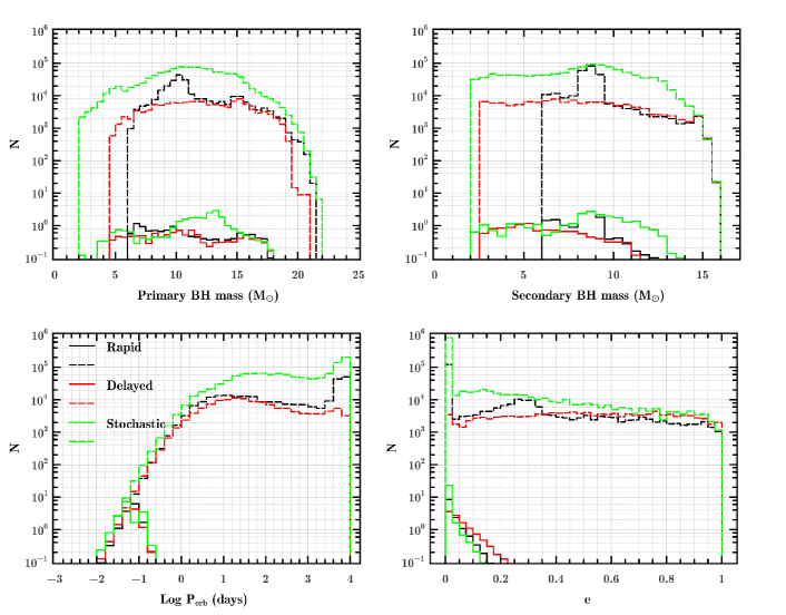
In Figure 6 we present similar histogram diagrams for calculated number distributions (solid curves) of LISA BHBH systems under different supernova models. For comparison, the dashed curves denote all Galactic BHBH binaries. The primary BHs tend to be heavier than the secondary ones, and have the maximal mass of in LISA BHBH binaries ( in all the Galactic binaries). The rapid model predicts that the secondary BHs of LISA binaries have the mass distribution in the range of with a peak which is similar to the case for the BH masses of LISA BHNS systems, while the other two models anticipate that a significant fraction of secondary BHs have masses within the mass gap. As most natal BHs are imparted by negligible kicks in the rapid and stochastic models, a large part of Galactic BHBH binaries have long periods of days in nearly circular orbits. In the delayed model, the orbital periods are mainly distributed in the range of days with a peak days, and the orbital eccentricities have a flat distribution between . Our calculations show that there are BHBH binaries detectable by LISA. Compared with the LISA BH binaries with an NS or a WD companion, these BHBH systems possess longer orbital periods up to day. Also, LISA BHBH binaries are expected to have relatively low eccentricities of .
4.4 GW detection of BHCS systems
Figure 7 shows predicted number distributions of detectable BHCS binaries by LISA in the plane for the rapid, delayed and stochastic models (from top to bottom panels). The left, middle and right panels correspond to the CS companion being a WD, an NS and a BH, respectively. In each panel, we have labelled the predicted number of the corresponding GW sources and the fraction of systems hosting BHs within the mass gap. In the rapid model, there are no mass-gap BHs produced, so are always zero for all three types of BHCS binaries. Both the delayed and the stochastic models predict that all BHWD binaries detectable by LISA possess a mass-gap BH, i.e. , and that decreases to and for BHNS and BHBH binaries, respectively. In the rapid model, all BHWD binaries have wide orbits and do not appear to be LISA sources. In the delayed and the stochastic models, BHWD systems cover two regions that correspond to detached systems (with relatively high values) and UCXBs (with relatively low values).

In Figure 8 we show the calculated number distributions of detectable BHCS binaries by LISA for all our adopted models, as a function of the chirp mass. In both the delayed and the stochastic models, LISA BHWD binaries can be divided into detached systems with and UCXBs with . For BHNS binaries, the chirp mass distributions can cover the range of , with an overlap between between the three models. LISA BHBH binaries have chirp masses mainly distributed in the range of for the delayed and stochastic models, and for the rapid model. Based on the chirp mass distributions for different types of BHCS binaries, LISA may distinguish BHBH systems if and BHWD systems if from BHNS binaries. However, the identification of BHCS binaries solely from GW observations is difficult since they can be confused with other types of GW sources such as NSNS systems and NSWD systems (see also Sesana et al., 2020, for the discussion on the identification of BH–BH binaries).
5 Populations of BHCS mergers in the local Universe
To estimate the merger rate density of the BHCS binaries in the local Universe, we have evolved a large number () of the primordial binaries for each model. The metallicity Z for every primordial binary is randomly taken in the logarithmic space between 0.0001 and 0.02. After simulations, we record relevant information for the BHCS binaries that can merge within the Hubble time, including the CS types, the component masses and the delay time (from the formation of the primordial binaries to the merger of the BHCS binaries). For each BHCS merger, the look back time of the merger can be estimated as
| (21) |
where is the look back time for (binary) stars formed at redshift ,
| (22) |
where , and are the cosmological parameters for which we adopt the values from Planck Collaboration et al. (2016). Following Mapelli et al. (2017), we consider the BHCS mergers with , excluding the systems that will merge in the future. And, we only include the mergers in the local Universe (defined as ) using the condition of . We further divide the recorded binaries into 20 logarithmically spaced metallicity bins between for each model. The metallicity for stars at a given redshift is computed as if and if (Rafelski et al., 2012). For or , we instead use the recorded information of the systems with or . In each metallicity bin, the parameter distribution of the primordial binaries has been normalized to unity. Similar to the treatment of Giacobbo & Mapelli (2018), we use the following analytic equation to calculate as (see also Spera et al., 2019)
| (23) |
where is the cosmic star-formation rate density as a function of redshift for which we use the fitted formula given by Madau & Dickinson (2014),
| (24) |
5.1 The BH–CS mergers with(out) mass-gap BHs
In Table 1, we show the predicted local merger rate densities of different types of BH–CS binaries and the fraction of the merging binaries that host mass-gap BHs for all our adopted models. The delayed and stochastic models predict and , respectively. The local merger rate densities of BH–NS binaries are in the range of , consistent with the inferred upper limit of from the LIGO/Virgo data444More recently, Abbott et al. (2021) reported the detection of two BH–NS mergers (GW200105 and GW200115) and inferred the merger rate density of if assuming they are representative of the BH–NS population. In this case, our calculated results can still match the observations. (Abbott et al., 2019). For BH–BH binaries, the merger rate densities are in the range of , slightly larger than the one given by LIGO/Virgo observations (Abbott et al., 2020b). Our obtained rates are obviously subject to many uncertainties such as the assumptions on supernova kicks, CE ejection efficiencies, stellar winds, and initial parameter distribution of the primordial binaries. For example, the calculated may better match observations if increasing the magnitude of the kick velocities for BHs. Compared with BH–CS mergers in the rapid model, we estimate that () of BH–WD mergers, () of BH–NS mergers, and () of BH–BH mergers host mass-gap BHs in the delayed (stochastic) model. We can see that these fractions are very close to those for the corresponding type of LISA binaries in the Milky Way.

Figure 9 shows the fractions of the BH–CS mergers with mass-gap BHs among all mergers as a function of the metallicity. We find that is not strongly dependent on metallicity. Both the delayed and the stochastic models predict that for BH–WD mergers, for BH–NS mergers, and for BH–BH mergers.

Figure 10 shows the component masses of the BHCS systems merged in the local Universe for all our adopted models. The black, red and green circles correspond to the CS companions being WDs, NSs and BHs, respectively. The blue star marks the position of GW190814. We can see that GW190814 cannot form in the rapid model if its less-massive component is a mass-gap BH. Predictably, some BH–BH binaries can match the component masses of GW190814-like systems in both the delayed and stochastic models. The formation of GW190814-like sources has been explored by Zevin et al. (2020), who suggest that the predicted rate of such mergers is in tension with the empirical LIGO/Virgo rate of other CS pair mergers if only involving isolated binary evolution channel.
Based on our calculated outcomes, it is possible to form BHNS systems where the NS forms first in the delayed and stochastic models (see Figure 10 for the binaries with primary mass ), but the merger rate of these binaries is orders of magnitude lower than that of the systems where the BH forms first. In the stochastic model, even a WD can form first in BHWD systems. Mass transfer efficiency during the primordial binary evolution is a vital factor to determinate whether the NS/WD can be formed before the BH (Sipior et al., 2004). Since we adopt the rotation-dependent mass transfer mode in our calculations, the relatively low mass-transfer efficiency makes it difficult to form the NS/WD before the BH.
5.2 Formation channels of BH–CS mergers
From the evolutionary point of view, BH–CS systems form either from stable mass transfer channel or the CE channel. Considering the evolution of the BH binaries with nondegenerate donors experienced either a stable mass transfer phase or a CE phase, we identify two channels for the formation of BHCS systems. Almost all BH–WD mergers are produced from the CE channel. About of BH–NS mergers are formed through the stable mass transfer channel, with the merger rate densities , and in the rapid, delayed and stochastic model, respectively. About of the BHBH mergers form from the stable mass transfer channel, with , and in the rapid, delayed and stochastic model, respectively. The contribution of the stable mass transfer channel stems from our revised CE criteria of mass transfer stability for the BH binaries with nondegenerate donors which allow large parameter spaces for stable mass transfer (see Section 3). In Figure 11, we schematically show the formation history of a BHBH merger containing a mass-gap BH through the evolutionary channel without any CE phase. The binary evolution starts from a primordial system consisting of a primary star and a secondary star in a 10 day orbit. The metallicity of both stars is initially taken to be 0.001. At the time of 6.6 Myr, the primary star, which has climbed to the supergiant branch, starts to overflow its RL. After about 0.3 Myr of stable mass transfer, the primary is stripped to be a Wolf-Rayet star and the secondary is rejuvenated by accretion of matter. The mass transfer efficiency is about 0.1 during this phase, with the rotation-dependent mode. When the Wolf-Rayet star collapses into a BH, the binary evolves to be an eccentric () system in a day orbit. At the time of 9.5 Myr, the secondary star overflows its RL and transfers mass to the BH, causing the binary orbit to shrink rapidly. The post-mass transfer system possesses a BH and a Wolf-Rayet star in a nearly circular orbit with a period of 5.2 days. After 0.3 Myr, a close BHBH system is formed and the second born BH has a mass of . About 9 Gyr later, this binary will merge to be a single BH.


5.3 Mass ratios and total masses of BH–CS mergers
Figure 12 shows the merger rate density distributions of the BHCS mergers in the local Universe, as a function of the mass ratio (of the light to the heavy components) and the total mass. (1) Since almost all BHWD mergers possess a mass-gap BH and the WDs have mass , both the delayed and the stochastic models predict that the mass ratios of such mergers are mainly distributed in the range of . Meanwhile, their total masses are expected to vary in a narrow range of . (2) In the rapid model, the BHNS mergers have the mass ratio distribution in the range of with a peak at and the total mass distribution in the range of with a peak at . Compared with the rapid model, the peak of the mass ratio distribution for BHNS mergers shifts to larger values of () and the peak of the total mass distribution to lower mass of () in the delayed (stochastic) model. (3) The BHBH mergers in the rapid and stochastic models tend to have large mass ratios whose distribution has a broad peak at and , respectively, while the delayed model has a relatively flat mass ratio distribution between . The total masses of the BHBH mergers in the rapid model are always larger than , but can extend down to in the delayed and stochastic models. After the detection of GW190412, the percentage of the BHBH mergers with mass ratios less than 0.4 has been constrained to constitute of the whole BHBH merger population (Abbott et al., 2020c). We estimate that the fractions are , and in the rapid, delayed and stochastic models, respectively. We do not further discuss the distribution shape (a broken power-law function) for the component masses of BHBH mergers (Abbott et al., 2020b), since one can revise the input physics (e.g. BH natal kicks and CE ejection efficiencies) to match the LIGO/Virgo data (see e.g., Olejak et al., 2021).
6 Conclusions
In this paper, we have investigated the properties of merging BHCS binary population in the Milky Way and the local Universe, based on binary evolution calculations with the BSE and MESA codes. Only the systems formed through isolated binary evolution are taken into account. Compared with previous works, the innovations in this work mainly lie in two aspects. (1) We have revised the criteria for the occurrence of CE evolution in the BH binaries with nondegenerate donors, by a large grid of detailed binary evolution simulations with the MESA code. As a consequence, we obtain the potential parameter space for dynamically (un)stable mass transfer, and incorporate into our BPS calculations. (2) We consider various mechanisms for the formation of NSs and BHs. The (non)existence of the mass gap between NSs and BHs is crucial to constrain the mechanism of supernova explosions. We adopt three models to deal with the compact remnant masses and natal kicks during supernova explosions, that is the rapid mechanism (Fryer et al., 2012), the delayed mechanism (Fryer et al., 2012) and the stochastic recipe (Mandel & Müller, 2020). The delayed and the stochastic models allow the formation of CSs within the mass gap, while the rapid model naturally leads to the mass gap between NSs and BHs. The fractions of merging systems with mass-gap BHs among the whole population for different types of BHCS systems can be used as an indicator to examine relevant supernova mechanisms. In the rapid model, always holds.
We identify two formation channels for close BHCS systems that appear as GW sources, depending on whether the mass transfer in the progenitor BH binaries is stable. We find that almost all close BHWD binaries have experienced a CE phase, during which a mass-gap BH was engulfed by the envelope of a supergiant (the WD’s progenitor). So for merging BHWD systems, we expect that in both the delayed and the stochastic models. For merging BHNS and BHBH systems, both the CE and stable mass transfer channels take effect. In both the delayed and stochastic models, we obtain that for merging BHNS binaries and for merging BHBH binaries. It seems that our predictions for merging BHCS binary population cannot make a clear distinction between the delayed and the stochastic models. The LIGO/Virgo operation will provide a rapid growing sample of BHBH merger events. For BHBH mergers with total mass , the delayed model anticipates a more flat mass-ratio distribution between while the stochastic model favors large mass ratios distributed with a broad peak at (see Figure 12).
We estimate that there are totally dozens of BHCS systems detectable by LISA in the Milky Way, and the merger rate density of BHCS systems varies in the range of in the local Universe. For merging BHWD binaries, the delayed and stochastic models predict and systems may be observed by LISA in the Milky Way, respectively. In addition, we expect that local BHWD merger rate is in the range of for the delayed and stochastic models. Our calculations show that BHNS systems are potential GW sources in the Milky Way and the local merger rate of BHNS binaries is in the range of . Among all Galactic BHBH systems, of them are expected to be the GW sources in the LISA frequency. Our calculated merger rate of BHBH binaries in the local Universe varies in the range of . At last we remind that our results are still subject to many uncertainties, including the assumption of binary fraction (), the treatments of stellar and binary evolutionary processes (see e.g., Langer, 2012), the options of Galactic and cosmological parameters, and etc. It is obvious that from observations (Moe & Di Stefano, 2017) can lead to the decrease of the LISA-detectable numbers and the local rates for the merging BH–CS binary populations.
References
- Aasi et al. (2015) Aasi, J., Abbott, B. P., Abbott, R. et al. 2015, Class. Quantum Grav., 32, 074001
- Abbott et al. (2016) Abbott, B. P., Abbott, R., Abbott, T. D., et al. 2016, Phys. Rev. Lett., 116, 061102
- Abbott et al. (2019) Abbott, B. P., Abbott, R., Abbott, T. D., et al. 2019, Phys. Rev. X, 9, 031040
- Abbott et al. (2020a) Abbott, R., Abbott, T. D., Abraham, S. et al. 2020a, ApJ, 896, L44
- Abbott et al. (2020b) Abbott, R., Abbott, T. D., Abraham, S. et al. 2020b, arXiv: 2010.14533
- Abbott et al. (2020c) Abbott, R., Abbott, T. D., Abraham, S. et al. 2020c, arXiv: 2004.08342
- Abbott et al. (2021) Abbott, R., Abbott, T. D., Abraham, S. et al. 2021, ApJ, 915, L5
- Abt (1983) Abt, H. A. 1983, ARA&A, 21, 343
- Acernese et al. (2015) Acernese, F., Agathos, M., Agatsuma, K. et al. 2015, Class. Quantum Grav., 32, 024001
- Alsing et al. (2018) Alsing, J., Silva, H. O., & Berti, E., 2018, MNRAS, 478, 1377
- Amaro-Seoane et al. (2017) Amaro-Seoane, P., Audley, H., Babak, S. et al. 2017, arXiv: 1702.00786
- Andrews et al. (2019) Andrews, J. J., Breivik, K., & Chatterjee, S. 2019, ApJ, 886, 68
- Antoniadis et al. (2013) Antoniadis, J., Freire, P., Wex, N., et al. 2013, Science, 340, 448
- Antonini & Rasio (2016) Antonini, F., & Rasio, F. A. 2016, ApJ, 831, 187
- Askar et al. (2017) Askar, A., Szkudlarek, M., Gondek-Rosińska, D., Giersz, M., & Bulik, T. 2017, MNRAS, 464, L36
- Bailyn et al. (1998) Bailyn, C. D., Jain, R. K., Coppi, P., & Orosz, J. A. 1998, ApJ, 499, 367
- Banerjee (2020) Banerjee, S. 2020, PhRvD, 102, 103002
- Barack & Cutler (2004) Barack, L., & Cutler, C. 2004, PhRvD, 70, 122002
- Bavera et al. (2021) Bavera, S. S., Fragos, T., Zevin, M. et al. 2021, A&A, 647, 153
- Begelman (1979) Begelman, M. C. 1979, MNRAS, 187, 237
- Belczynski et al. (2008) Belczynski, K., Kalogera, V., Rasio, F., et al. 2008, ApJS, 174, 223
- Belczynski et al. (2010) Belczynski, K., Bulik, T., Fryer, C., et al 2010, ApJ, 714, 1217
- Belczynski et al. (2016) Belczynski, K., Holz, D. E., Bulik, T., & O’Shaughnessy, R., 2016, Nature, 534, 512
- Breivik et al. (2017) Breivik, K., Chatterjee, S., & Larson, S. L. 2017, ApJL, 850, L13
- Breivik et al. (2019) Breivik, K., Chatterjee, S., & Andrews, J. J. 2019, ApJ, 878, L4
- Breivik et al. (2020) Breivik, K., Coughlin, S., Zevin, M., et al. 2020, ApJ, 898, 71
- Broekgaarden et al. (2021) Broekgaarden, F. S., Berger, E., Neijssel, C. J., et al. 2021, arXiv: 2103.02608
- Brott et al. (2011) Brott, I., de Mink, S. E., Cantiello, M., et al. 2011, A&A, 530, 115
- Chattopadhyay et al. (2020) Chattopadhyay, D., Stevenson, S., Hurley, J. R., Bailes, M., & Broekgaarden, F., 2020, arXiv: 2011.13503
- Chen et al. (2020) Chen, W.-C., Liu, D.-D., Wang, B. 2020, ApJ, 900, L8
- Copperwheat et al. (2016) Copperwheat, C. M., Steele, I. A., Piascik, A. S., et al. 2016, MNRAS, 462, 3528
- de Mink & Mandel (2016) de Mink, S. E., & Mandel, I. 2016, MNRAS, 460, 3545
- Dessart et al. (2006) Dessart, L., Burrows, A., Ott, C. D., et al. 2006, ApJ, 644, 1063
- Di Carlo et al. (2019) Di Carlo, U. N., Giacobbo, N., Mapelli, M., et al. 2019, MNRAS, 487, 2947
- Diehl et al. (2006) Diehl, R., Halloin, H., Kretschmer, K., et al. 2006, Nature, 439, 45
- Dong et al. (2018) Dong, Y.-Z., Gu, W.-M., Liu, T., & Wang, J. 2018, MNRAS, 475, L101
- Downing et al. (2010) Downing, J. M. B., Benacquista, M. J., Giersz, M., & Spurzem, R., 2010, MNRAS, 407, 1946
- Eldridge & Stanway (2016) Eldridge, J. J., & Stanway, E. R. 2016, MNRAS, 462, 3302
- Farr et al. (2011) Farr, W. M., Sravan, N., Cantrell, A., et al. 2011, ApJ, 741, 103
- Farr & Chatziioannou (2020) Farr, W. M., & Chatziioannou, K. 2020, Res. Notes Am. Astron. Soc., 4, 65
- Feast & Whitelock (1997) Feast, M., & Whitelock, P. 1997, MNRAS, 291, 683
- Fragione et al. (2020) Fragione, G., Metzger, B. D., Perna, R., Leigh, N. W. C., Kocsis, B. 2020, MNRAS, 495, 1061
- Fragione & Loeb (2019) Fragione, G., & Loeb, A. 2019, MNRAS, 490, 4991
- Fryer et al. (2012) Fryer, C., Belczynski, K., Wiktorowicz, G., et al. 2012, ApJ, 749, 91
- Giacobbo & Mapelli (2018) Giacobbo, N., & Mapelli, M. 2018, MNRAS, 480, 2011
- Ge et al. (2010) Ge, H., Hjellming, M. S., Webbink, R. F., Chen, X., & Han, Z. 2010, ApJ, 717, 724
- Ge et al. (2020) Ge, H., Webbink, R., & Han, Z. 2020, ApJS, 249, 9
- Gompertz et al. (2020) Gompertz, B. P., Levan, A. J., & Tanvir N. R. 2020, ApJ, 895, 58
- Gould & Salim (2002) Gould, A., & Salim, S. 2002, ApJ, 572, 944
- Hamann et al. (1995) Hamann, W.-R., Koesterke, L., & Wessolowski, U., 1995, A&A, 299, 151
- Han et al. (2020a) Han, M.-Z., Tang, S.-P., Hu, Y.-M., Li, Y.-J., Jiang, J.-L., Jin, Z.-P., Fan, Y.-Z., & Wei, D.-M. 2020a, ApJ, 891, L5
- Han et al. (2020b) Han, Z.-W., Ge, H.-W., Chen, X.-F., & Chen, H.-L. 2020b, RAA, 20, 161
- Hoang et al. (2018) Hoang, B.-M., Naoz, S., Kocsis, B., Rasio, F. A., & Dosopoulou, F. 2018, ApJ, 856, 140
- Hobbs et al. (2005) Hobbs, G., Lorimer, D. R., Lyne, A. G., & Kramer, M. 2005, MNRAS, 360, 974
- Hotokezaka et al. (2016) Hotokezaka, K., Nissanke, S., Hallinan, G., et al. 2016, ApJ, 831, 190
- Huang et al. (2020) Huang, K., Hu, J., Zhang, Y., & Shen, H. 2020, ApJ, 904, 39
- Hurley et al. (2002) Hurley, J. R., Tout, C. A., & Pols, O. R. 2002, MNRAS, 329, 897
- Iben & Livio (1993) Iben, I. J., & Livio, M. 1993, PASP, 105, 1373
- Ivanova et al. (2010) Ivanova, N., Chaichenets, S., Fregeau, J., et al. 2010, ApJ, 717, 948
- Ivanova et al. (2013) Ivanova, N., Justham, S., Chen, X., et al. 2013, A&AR, 21, 59
- Jayasinghe et al. (2021) Jayasinghe, T., Stanek, K. Z., Thompson, T. A. et al. 2021, MNRAS, 504, 2577
- Kiel & Hurley (2006) Kiel, P. D., & Hurley, J. R., 2006, MNRAS, 369, 1152
- King & Begelman (1999) King, A. R., & Begelman, M. C. 1999, ApJ, 519, L169
- Kinugawa et al. (2014) Kinugawa, T., Inayoshi, K., Hotokezaka, K., Nakauchi, D., & Nakamura, T. 2014, MNRAS, 442, 2963
- Klencki et al. (2018) Klencki, J., Moe, M., Gladysz, W., et al. 2018, A&A, 619, 77
- Klencki et al. (2021) Klencki, J., Nelemans, G., Istrate, A. G., & Chruslinska, M. 2021, A&A, 645, 54
- Kobulnicky & Fryer (2007) Kobulnicky, H. A., & Fryer, C. L. 2007, ApJ, 670, 747
- Kobulnicky et al. (2014) Kobulnicky, H. A., Kiminki, D. C., Lundquist, M. J., et al. 2014, ApJS, 213, 34
- Kolb & Ritter (1990) Kolb, U., & Ritter, H. 1990, A&A, 236, 385
- Kolb et al. (2000) Kolb, U., Davies, M. B., King, A., & Ritter, H. 2000, MNRAS, 317, 438
- Kremer et al. (2017) Kremer, K., Breivik, K., Larson, S. L., & Kalogera, V. 2017, ApJ, 846, 95
- Kremer et al. (2019) Kremer, K., Rodriguez, C. L., Amaro-Seoane, P. et al. 2019, PhRvD, 99, 063003
- Kremer et al. (2020) Kremer, K., Ye, C. S., Rui, N. Z., et al. 2020, ApJS, 247, 48
- Kroupa et al. (1993) Kroupa, P., Tout, C. A., & Gilmore, G. 1993, MNRAS, 262, 545
- Kyutoku et al. (2020) Kyutoku, K., Fujibayashi, S., Hayashi, K., et al. 2020, ApJ, 890, L4
- Lamberts et al. (2018) Lamberts, A., Garrison-Kimmel, S., Hopkins, P. F., et al. 2018, MNRAS, 480, 2704
- Langer (2012) Langer, N. 2012, ARA&A, 50, 107
- Lau et al. (2020) Lau, M. Y. M., Mandel, I., Vigna-Gómez, A. et al. 2020, MNRAS, 492, 3061
- Li & Paczyński (1998) Li, L.-X., & Paczyński, B. 1998, ApJ, 507, L59
- Lipunov et al. (1997) Lipunov, V. M., Postnov, K. A., & Prokhorov, M. E. 1997, Astronomy Letters, 23, 492
- Liu & Lai (2018) Liu, B. & Lai, D. 2018, ApJ, 863, 68
- Luo et al. (2016) Luo, J., Chen, L., Duan, H. et al., 2016, Class. Quantum Grav., 33, 035010
- Maccarone et al. (2007) Maccarone, T. J., Kundu, A., Zepf, S. E., & Rhode, K. L. 2007, Natur, 445, 183
- Madau & Dickinson (2014) Madau, P., & Dickinson, M. 2014, ARA&A, 52, 415
- Mandel & de Mink (2016) Mandel, I., & de Mink, S. E. 2016, MNRAS, 458, 2634
- Mandel & Müller (2020) Mandel, I., & Müller, B. 2020, MNRAS, 499, 3214
- Mapelli et al. (2017) Mapelli, M., Giacobbo, N., Ripamonti, E., & Spera, M. 2017, MNRAS, 472, 2422
- Mapelli & Giacobbo (2018) Mapelli, M., & Giacobbo, N. 2018, MNRAS, 479, 4391
- Marchant et al. (2016) Marchant, P., Langer, N., Podsiadlowski, P., Tauris, T. M., & Moriya, T. J. 2016, A&A, 588, A50
- Marchant et al. (2021) Marchant, P., Pappas, K. M. W., Gallegos-Garcia, M. et al. 2021, arXiv: 2103.09243
- Margalit & Metzger (2017) Margalit, B., & Metzger, B. D. 2017, ApJ, 850, L19
- Mashian & Loeb (2017) Mashian, N., & Loeb, A. 2017, MNRAS, 470, 2611
- McKernan et al. (2018) McKernan, B., Ford, K. E. S., Bellovary, J., et al. 2018, ApJ, 866, 66
- Metzger (2012) Metzger, B. D. 2012, MNRAS, 419, 827
- Miller-Jones et al. (2015) Miller-Jones, J. C. A., Strader, J., Heinke, C. O., et al. 2015, MNRAS, 453, 3918
- Misra et al. (2020) Misra, D., Fragos, T., Tauris, T. M., Zapartas, E., & Aguilera-Dena, D. R. 2020, A&A, 642, 174
- Moe & Di Stefano (2017) Moe, M.,& Di Stefano, R., 2017, ApJS, 230, 15
- Nakar & Piran (2011) Nakar E., & Piran T. 2011, Nature, 478, 82
- Nelemans et al. (2004) Nelemans, G., Yungelson, L. R., Portegies Zwart, S. F. 2004, MNRAS, 349, 181
- Nieuwenhuijzen & de Jager (1990) Nieuwenhuijzen, H., & de Jager, C. 1990, A&A, 231, 134
- O’Leary et al. (2009) O’Leary, R. M., Kocsis, B., & Loeb, A. 2009, MNRAS, 395, 2127
- Olejak et al. (2021) Olejak, A., Belczynski, K., & Ivanova, N. 2021, arXiv: 2102.05649
- Özel et al. (2010) Özel, F., Psaltis, D., Narayan, R., & McClintock, J. E. 2010, ApJ, 725, 1918
- Paczynski (1976) Paczynski, B. 1976, in Proc. IAU Symp. 73, Structure and Evolution in Close Binary Systems, ed. P. P. Eggleton, S. Mitton & J. Whealan (Dordrecht: Reidel), 75
- Paczynski (1986) Paczynski, B. 1986, ApJL, 308, L43
- Pavlovskii & Ivanova (2015) Pavlovskii, K. & Ivanova, N. 2015, MNRAS, 449, 4415
- Pavlovskii et al. (2017) Pavlovskii, K., Ivanova, N., Belczynski, K. & Van, K. X. 2017, MNRAS, 465, 2092
- Paxton et al. (2011) Paxton, B., Bildsten, L., Dotter, A., et al. 2011, ApJS, 192, 3
- Paxton et al. (2013) Paxton, B., Cantiello, M., Arras, P., et al. 2013, ApJS, 208, 4
- Paxton et al. (2015) Paxton, B., Marchant, P., Schwab, J., et al. 2015, ApJS, 220, 15
- Paxton et al. (2018) Paxton, B., Schwab, J., Bauer, E. B., et al. 2018, ApJS, 234, 34
- Paxton et al. (2019) Paxton, B., Smolec, R., Schwab, J., et al. 2019, ApJS, 243, 10
- Perna et al. (2019) Perna, R., Wang, Y.-H., Farr, W. M., Leigh, N., & Cantiello, M. 2019, ApJ, 878, L1
- Peters & Mathews (1963) Peters, P. C., & Mathews, J. 1963, PhRv, 131, 435
- Planck Collaboration et al. (2016) Planck Collaboration, Ade, P. A. R., Aghanim, N. et al. 2016, A&A, 594, 13
- Podsiadlowski et al. (2002) Podsiadlowski, Ph., Rappaport, S., & Pfahl, E. D. 2002, ApJ, 565, 1107
- Racusin et al. (2017) Racusin, J. L., Burns, E., Goldstein, A., et al. 2017, ApJ, 835, 82
- Rafelski et al. (2012) Rafelski, M., Wolfe, A. M., Prochaska, J. X., Neeleman, M., & Mendez, A. J. 2012, ApJ, 755, 89
- Raithel et al. (2018) Raithel, C. A., Sukhbold, T., & Özel, F. 2018, ApJ, 856, 35
- Rastello et al. (2020) Rastello, S., Mapelli, M., Di Carlo, U. N., et al. 2020, MNRAS, 497, 1563
- Robitaille & Whitney (2010) Robitaille, T. P., & Whitney, B. A. 2010, ApJL, 710, L11
- Robson et al. (2019) Robson, T., Cornish, N. J., & Liu, C. 2019, CQGra, 36, 105011
- Rodriguez et al. (2016) Rodriguez, C. L., Haster, C.-J., Chatterjee, S., Kalogera, V., & Rasio, F. A. 2016, ApJ, 824, L8
- Ruan et al. (2020) Ruan, W.-H., Guo, Z.-K., Cai, R.-G., & Zhang, Y.-Z., 2020, Int. J. Mod. Phys. A, 35, 2050075
- Ruiz et al. (2018) Ruiz, M., Shapiro, S. L., & Tsokaros, A., 2018, Phys. Rev., D, 97, 021501
- Sana et al. (2012) Sana, H., de Mink, S. E., de Koter, A., et al. 2012, Science, 337, 444
- Santoliquido et al. (2020) Santoliquido, F., Mapelli, M., Bouffanais Y., et al. 2020, ApJ, 898, 152
- Sberna et al. (2021) Sberna, L., Toubiana, A., & Miller, M. C. 2021, ApJ, 908, 1
- Sesana et al. (2020) Sesana, A., Lamberts, A., & Petiteau, A. 2020, MNRAS, 494, L75
- Smith et al. (1978) Smith, L. F., Biermann, P., & Mezger, P. G. 1978, A&A, 66, 65
- Shibata et al. (2019) Shibata, M., Zhou, E., Kiuchi, K., & Fujibayashi, S., 2019, Phys. Rev., D, 100, 023015
- Shao & Li (2012) Shao, Y., & Li, X.-D. 2012, ApJ, 756, 85
- Shao & Li (2014) Shao, Y., & Li, X.-D. 2014, ApJ, 796, 37
- Shao & Li (2016) Shao, Y., & Li, X.-D. 2016, ApJ, 833, 108
- Shao & Li (2018) Shao, Y., & Li, X.-D. 2018, MNRAS, 477, L128
- Shao & Li (2019) Shao, Y., & Li, X.-D. 2019, ApJ, 885, 151
- Shao & Li (2020) Shao, Y., & Li, X.-D. 2020, ApJ, 898, 143
- Silsbee & Tremaine (2017) Silsbee, K., & Tremaine, S. 2017, ApJ, 836, 39
- Sipior et al. (2004) Sipior, M. S., Portegies Zwart, S., & Nelemans, G. 2004, MNRAS, 354, L49
- Smartt et al. (2016) Smartt, S. J., Chambers, K. C., Smith, K. W., et al. 2016, ApJ, 827, L40
- Soberman et al. (1997) Soberman, G. E., Phinney, E. S., & van den Heuvel, E. P. J. 1997, A&A, 327, 620
- Spera et al. (2019) Spera, M., Mapelli, M., Giacobbo, N., et al. 2019, MNRAS, 485, 889
- Stevenson et al. (2017) Stevenson, S., Vigna-Gómez, A., Mandel, I., et al. 2017, Nature Communications, 8, 14906
- Stone et al. (2017) Stone, N. C., Metzger, B. D., & Haiman, Z. 2017, MNRAS, 464, 946
- Sukhbold et al. (2016) Sukhbold, T., Ertl, T., Woosley, S. E., Brown, J. M., & Janka, H.-T. 2016, ApJ, 821, 38
- Stancliffe & Eldridge (2009) Stancliffe, R. & Eldridge, J. 2009, MNRAS, 396, 1699
- Tanikawa et al. (2021) Tanikawa, A., Susa, H., Yoshida, T., Trani, A. A., & Kinugawa, T. 2021, ApJ, 910, 30
- Tauris et al. (2000) Tauris, T. M., van den Heuvel, E. P. J., & Savonije, G. J. 2000, ApJ, 530, L93
- Tauris et al. (2015) Tauris, T., Langer, N., & Podsiadlowski, P. 2015, MNRAS, 451, 2123
- Tauris (2018) Tauris, T. M. 2018, PhRvL, 121, 131105
- Thompson et al. (2019) Thompson, T. A., Kochanek, C. S., Stanek, K. Z., et al. 2019, Science, 366, 637
- Timmes et al. (1996) Timmes, F. X., Woosley, S. E., & Weaver, T. A. 1996, ApJ, 457, 834
- Tout et al. (1996) Tout, C. A., Pols, O. R., Eggleton, P. P., & Han, Z. 1996, MNRAS, 281, 257
- Tutukov & Yungelson (1993) Tutukov, A. V. & Yungelson, L. R. 1993, MNRAS, 260, 675
- van den Heuvel et al. (2017) van den Heuvel, E. P. J., Portegies Zwart, S. F., de Mink, S. E. 2017, MNRAS, 471, 4256
- van Haaften et al. (2012) van Haaften, L. M., Nelemans, G., Voss, R., Wood, M. A., & Kuijpers, J. 2012, A&A, 537, A104
- Vink et al. (2001) Vink, J. S., de Koter, A., & Lamers, H. J. G. L. M. 2001, A&A, 369, 574
- Voss & Tauris (2003) Voss, R. & Tauris, T. M. 2003, MNRAS, 342, 1169
- Wang et al. (2021) Wang, B., Chen, W., Liu, D., et al 2021, arXiv: 2106.01369
- Webbink (1984) Webbink, R. F. 1984, ApJ, 277, 355
- Wen (2003) Wen, L. 2003, ApJ, 598, 419
- Wiktorowicz et al. (2020) Wiktorowicz, G., Lu, Y., Wyrzykowski, Ł. 2020, ApJ, 905, 134
- Wyrzykowski & Mandel (2020) Wyrzykowski, Ł., & Mandel, I. 2020, A&A, 636, A20
- Xu & Li (2010) Xu, X.-J., & Li, X.-D. 2010, ApJ, 716, 114
- Yalinewich et al. (2018) Yalinewich, A., Beniamini, P., Hotokezaka, K., & Zhu, W. 2018, MNRAS, 481, 930
- Yamaguchi et al. (2018) Yamaguchi, M. S., Kawanaka, N., Bulik, T., & Piran, T. 2018, ApJ, 861, 21
- Zevin et al. (2020) Zevin, M., Spera, M., Berry, C. P. L., & Kalogera, V. 2020, ApJ, 899, L1
- Zhou et al. (2020) Zhou, X., Li, A., & Li, B.-A. 2020, arXiv: 2011.11934
- Zhu et al. (2020) Zhu, J.-P., Wu, S.,Yang, Y.-P., et al. 2020, arXiv: 2011.02717
- Ziosi et al. (2014) Ziosi, B. M., Mapelli, M., Branchesi, M., & Tormen, G. 2014, MNRAS, 441, 3703