Policy Distillation with Selective Input Gradient Regularization for Efficient Interpretability
Abstract
Although deep Reinforcement Learning (RL) has proven successful in a wide range of tasks, one challenge it faces is interpretability when applied to real-world problems. Saliency maps are frequently used to provide interpretability for deep neural networks. However, in the RL domain, existing saliency map approaches are either computationally expensive and thus cannot satisfy the real-time requirement of real-world scenarios or cannot produce interpretable saliency maps for RL policies. In this work, we propose an approach of Distillation with selective Input Gradient Regularization (DIGR) which uses policy distillation and input gradient regularization to produce new policies that achieve both high interpretability and computation efficiency in generating saliency maps. Our approach is also found to improve the robustness of RL policies to multiple adversarial attacks. We conduct experiments on three tasks, MiniGrid (Fetch Object), Atari (Breakout) and CARLA Autonomous Driving, to demonstrate the importance and effectiveness of our approach.
1 Introduction
Reinforcement learning (RL) systems have achieved impressive performance in a wide range of simulated domains such as games (Mnih et al., 2015; Silver et al., 2016; Vinyals et al., 2019) and robotics (Lillicrap et al., 2015; Fujimoto et al., 2018; Haarnoja et al., 2018). However, the interpretability of an agent’s decision making and robustness to attacks need to be addressed when applying RL to real-world problems. For instance, in a self-driving scenario, real-time interpretability could explain how an RL agent produces a decision in response to its observed states and enable a safer deployment under real-world conditions and adversarial attacks (Ferdowsi et al., 2018).
Saliency maps in deep learning is a technique used to interpret input features that are believed to be important for the neural network output (Simonyan et al., 2013; Selvaraju et al., 2017; Fong & Vedaldi, 2017; Smilkov et al., 2017; Sundararajan et al., 2017; Zhang et al., 2018). As the issue of interpretability in RL gets more attention, a number of methods have been proposed to generate saliency maps to explain the decision making of RL agents. Existing saliency map methods in RL either use gradients to estimate the influence of input features on the output (Wang et al., 2016) (gradient-based methods) or compute the saliency of an input feature by perturbing it and observing the change in output (Greydanus et al., 2018; Iyer et al., 2018; Puri et al., 2020) (perturbation-based methods). Gradient-based methods can compute saliency maps efficiently with backpropagation. However, the quality of gradient-based saliency maps is generally poor (Rosynski et al., 2020). Perturbation-based methods are effective in highlighting the important features of the input, but at a significant computationally cost, which can make them ineffective when deployed on systems with real-time constraints. As a result, existing RL agents cannot provide high interpretability in a computation-efficient manner.
Different from previous work proposing new saliency calculation methods, we focus on improving the natural interpretability of RL policies. Given a RL policy, we propose an approach of Distillation with selective Input Gradient Regularization (DIGR) that uses policy distillation and input gradient regularization to retrain a new policy. In our approach, input gradient regularization selectively regularizes gradient-based saliency maps of the policy to imitate its interpretable perturbation-based saliency maps. This allows the new RL policy to generate high-quality saliency maps with gradient-based methods and thus achieve both high interpretability and computational efficiency. At the same time, to ensure that input gradient regularization does not cause task performance degradation, we use policy distillation (Czarnecki et al., 2019) to constrain the output of the new RL policy to remain close to the original RL policy.
We evaluate our method in three different tasks, which include an object fetching task from MiniGrid (Chevalier-Boisvert et al., 2018), Breakout from Atari games and CARLA Autonomoud Driving (Dosovitskiy et al., 2017). The results show that RL policies trained with our approach are able to achieve efficient interpretability while maintaining good task performance. Selective input gradient regularization also improves the robustness of RL policies to adversarial attacks. These two desired properties allow the RL policy to better adapt to real-world scenarios.
To summarize, we demonstrate a novel approach to improve the efficient interpretability and robustness to attacks of RL policies based on the utilization of saliency maps. Our approach increases the applicability of RL to real-world problems.
2 Background and Motivation


Reinforcement Learning
In reinforcement learning, agents learn to take actions in an environment that maximize their cumulative rewards. The environment is typically stated in the form of a Markov Decision Process (MDP), which is expressed in terms of the tuple () where is the state space, is the action space, is the transition function and is the reward function. At each time step in the MDP, the agent takes an action in the environment based on current state and receives a reward and next state . The goal of the agent is to find a policy to select actions that maximize the discounted cumulative future rewards , where is the discount factor ranging from to .
Policy Distillation
Policy distillation (Rusu et al., 2015; Czarnecki et al., 2019) transfers knowledge from one teacher policy to a student policy by training the student policy to produce the same behavior as the teacher policy. This is normally achieved by supervised regression to minimize the following objective:
| (1) |
where is the control policy that interacts with the environment to produce states for training, and is a distance metric. There are multiple choices for both and . For example, the control policy could take the form of the teacher policy or student policy or even a combination of them. Suitable distance metrics could be mean squared error or KL divergence.
Saliency Map in RL
Saliency map techniques are popular in computer vision and RL communities for interpreting deep neural networks. Gradient-based methods calculate the gradient of some function with respect to inputs based on the chain rule and then use the gradients to estimate the influence of input features on the output. In RL, one common approach is the Jacobian saliency map (Wang et al., 2016) which computes the saliency of input feature as where function could be calculated from either the state-action value in Q-learning or the action distribution in actor-critic methods. Other gradient-based visualization methods from the field of image classification are also explored (Greydanus et al., 2018; Rosynski et al., 2020) but most of them didn’t work well in the RL domain.
Perturbation-based methods compute the saliency of an input feature by perturbing (e.g. removing, altering or masking) the feature and observing the change in output. Given a state input , a perturbed state could be generated by inducing a perturbation on input feature . The approach of computing the change in output caused by the perturbation may vary based the form of RL agent. For example, in Q-learning, the network output is a scalar and thus the saliency of could be defined as . In actor-critic methods, the saliency of could be defined as which is the KL divergence between action distributions before and after the perturbation. Alternatively, (Greydanus et al., 2018) considers the output of actor as a vector and computes the saliency as . Puri et al. (2020) further proposed an approach called SARFA to addresses the specificity and relevance in perturbation-based saliency maps.
Motivation
We first introduce a simple fetching-object task in MiniGrid and demonstrate the results of different saliency map methods on this task to motivate our method. In the fetching-object task in MiniGrid, the environment is a room composed of 8x8 grids and 4 entities with unique colors. The red agent needs to locate and pick up the green object, while the yellow and blue objects are distractors. Based on the task rule, we name this task as Red-Fetch-Green. We first use PPO (Schulman et al., 2017) to train a RL policy to solve the task and then investigate the interpretability and computation efficiency of different saliency map methods to explain the policy. Examples of gradient-based (Vanilla Gradient (Simonyan et al., 2013), Guided Backprop (Springenberg et al., 2014), Grad-CAM (Selvaraju et al., 2017), Integrated Gradient (Sundararajan et al., 2017), Smooth Gradient (Smilkov et al., 2017)) and perturbation-based (Gaussian-Blur Perturbation (Greydanus et al., 2018) and SARFA (Puri et al., 2020)) saliency maps for Red-Fetch-Green are shown in Figure 1(a). We also include an example of saliency map generated by our DIGR approach for comparison. In general, for methods except DIGR, perturbation-based saliency maps mainly demonstrate high saliency on task relevant features (e.g. red agent and green target object) while gradient-based saliency maps are more noisy and harder to interpret. However, the high quality of perturbation-based saliency maps are achieved with an increased cost of computation time as shown in Figure 1(b). The computation time of perturbation-based saliency maps are highly affected by the input size and policy network architectures. This makes it incompatible with many real-world tasks that require real-time interpretability such as autonomous driving. Thus, based on the result in Figure 1, we find that normal gradient-based saliency maps are computationally more efficient but hard to interpret while perturbation-based saliency maps are more interpretable but come with a higher computation cost during deployment. This finding motivates us to think about how we can keep the computation efficiency of gradient-based methods and high interpretability of perturbation-based methods while avoiding their limitations, and thus propose DIGR.
How does DIGR generate interpretable saliency maps like perturbation-based methods while only requiring a short generation time as the most efficient Vanilla Gradient saliency maps? Is it possible for us to use gradient-based methods such as Vanilla Gradient method to generate high-quality saliency maps as those from perturbation-based methods? We answer these questions in the next section.
3 Method
Our approach to achieve both computational efficiency and high interpretability in RL is to produce a policy whose gradient-based saliency maps are comparable to those of perturbation-based methods. To achieve this, given a trained RL policy, we set its perturbation-based saliency maps as supervisory signals and update the weights of the policy so that its gradient-based saliency maps match the perturbation-based saliency maps. Since the computations involved in gradient-based saliency maps are differentiable, we can use stochastic gradient descent to conduct the training. The idea of optimizing gradient-based saliency maps has a close connection with input gradient regularization which imposes constraints on how input gradients behaves. For example, Ross & Doshi-Velez (2018) penalizes input gradients based on expert annotation to prevent the network from “attending” to certain parts of the input in an image classification task. Inspired by this, the training of the gradient-based saliency map in our approach is conducted by selectively penalizing the gradients of input features that have low perturbation-based saliency.
One challenge of selective input gradient regularization is that optimizing gradient-based saliency maps may also affect the policy output and thus degrade the task performance. To avoid this, we conduct policy distillation to ensure that the new policy maintains the same task performance. We give a more formal introduction of our method below.
Given a RL policy and input , we define the function as the method used in generating gradient-based saliency map and function as the method used in generating perturbation-based saliency map . Both and have the same size as input . Each element in the saliency map, and , are computed as
| (2) | ||||
| (3) | ||||
where and compute the gradient-based and perturbation-based saliency values of input feature given policy . These saliency values are then normalized between 0 and 1 to form saliency maps which contain elements in each map. In this work, perturbation function induces a Gaussian blur on the input with the input feature of interest as the center (Greydanus et al., 2018). It’s worth mentioning that, besides perturbation-based saliency maps, DIGR could be easily extended to utilize other saliency data (e.g. saliency maps from expert annotation) as supervisory signals. In this work, we focus on using perturbation-based saliency maps for input gradient regularization as they show high interpretability and can be computed as long as we have access to the policy and states.
After introducing the process of generating two types of saliency maps given a RL policy and state input, we introduce how they are used in DIGR. Given a trained RL policy , DIGR aims to produce a new policy with parameters that can generate interpretable saliency maps using gradient-based method. Given a state input , the saliency map could differ based on the generation method (gradient-based vs perturbation-based) and the policy ( vs ) used to generate them. For clarity, we define these 4 types of saliency maps as , , , where and represent gradient-based and perturbation-based saliency maps, respectively. The superscripts and represent whether the saliency map is generated by the given trained policy or the new policy . Then the loss function for input gradient regularization is
| (4) |
where is the state distribution following policy and is the number of input features in the saliency map. and have the same size and are both indexed by . Threshold is used in the indicator function to determine whether one input gradient should be penalized. The indicator function returns 1 if and 0 otherwise. In other words, if the perturbation-based saliency for an input feature is below threshold , the loss penalizes its gradient-based saliency. This selective penalization allows the model to only keep high saliency on task-relevant features selected by the perturbation-based saliency maps.
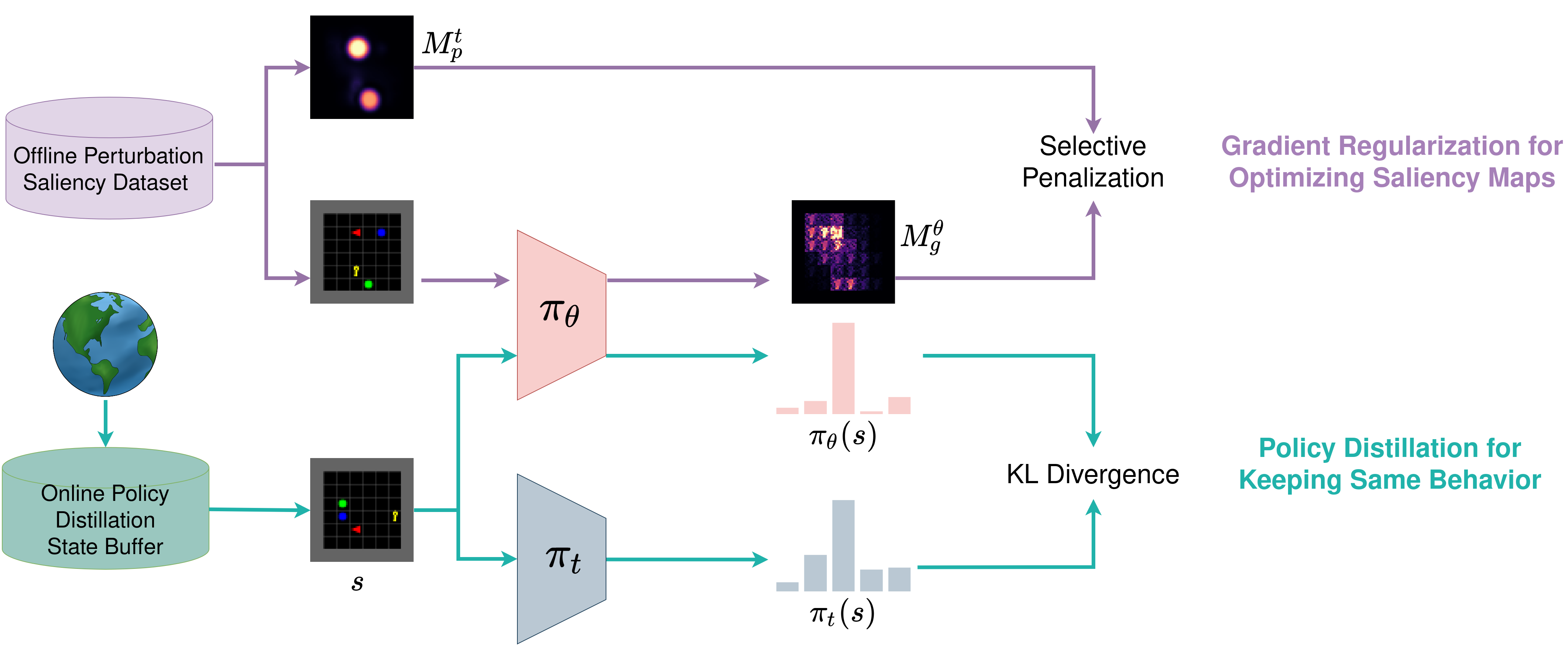
The final loss function in our approach is a weighted combination of selective input gradient regularization and policy distillation. In practice, generating perturbation-based saliency maps online for input gradient regularization could be time-consuming and slow down the overall training. To address this, we build an offline perturbation saliency dataset which contains states sampled from and the corresponding perturbation-based saliency maps generated in advance. Because of the policy similarity brought by policy distillation, we use to approximate for input gradient regularization. As a result, the loss function for DIGR is
| (5) | |||
where is a weighting parameter used to balance the loss of input gradient regularization and policy distillation. We show the complete architecture of our approach in Figure 2.
4 Experimental Results
We conducted experiments on three tasks including Red-Fetch-Green in MiniGrid, Breakout in Atari games and CARLA Autonomous Driving to demonstrate the effectiveness of our approach. In Red-Fetch-Green , the red agent needs to locate and pick up the green object while avoiding picking up other distractors in a room composed of 8x8 grids. In Breakout, the paddle is controlled to move at the bottom to ricochet the ball against the bricks and eliminate them for rewards. Besides these two tasks, we designed a CARLA Autonomous Driving task in which the agent needs to control an autonomous car driving on a highway while avoiding collisions. Since CARLA simulator has its simulation clock and time that can be matched with real time, we use it to demonstrate that both high quality and computation efficiency of our approach in interpreting RL policies are important in real-world scenarios.
4.1 Setup
RL Training
In our experiments, we first use PPO algorithm to train RL policies on Red-Fetch-Green, Breakout and CARLA Autonomous Driving. The trained RL policies, which are used to generate offline perturbation saliency datasets for input gradient regularization, also serve as the teacher policy in policy distillation and generate saliency maps for comparison. In all three tasks, we used similar network architectures composed of 3 convolutional layers and 2 linear layers but with different layer sizes. The trained RL policies achieved reasonable good performance in each task: The policy in Red-Fetch-Green solves the task with a success rate of 100%; the policy in Breakout achieves an average score of 320; the policy in CARLA Autonomous Driving could drive smoothly and learned to steer to avoid collision with other vehicles. We include more details of RL training in the appendix.
Offline Perturbation Saliency Dataset
To conduct selective input gradient regularization, we generate an offline perturbation saliency dataset by sampling states experienced by the trained RL policy and generating the corresponding Gaussian-Blur perturbation saliency maps (Greydanus et al., 2018). The perturbation saliency datasets of Red-Fetch-Green, Breakout and CARLA Autonomous Driving contain 1k, 10k, 2.5k pairs of states and saliency maps. Although our method still needs to generate perturbation-based saliency maps, the computation happens in the training stage without affecting the computation efficiency during deployment. Also, the computation problem could be mitigated by the limited size of the dataset (e.g. 1k, 10k and 2.5k states in Red-Fetch-Green, Breakout, and CARLA respectively) and the potential utilization of parallel computing with multiple machines.
DIGR Training
DIGR uses selective input gradient regularization and policy distillation to produce a new policy that achieves efficient interpretability while maintaining task performance. In all three experiments, we randomly initiate the new policy . To further stabilize the training, we consider the training of selective input gradient regularization and policy distillation as a multi-objective optimization problem and used the technique of PCGrad (Yu et al., 2020) to mitigate gradient interference. More hyperparameters of training are included in the appendix.
4.2 Effectiveness via Visual Illustrative Examples


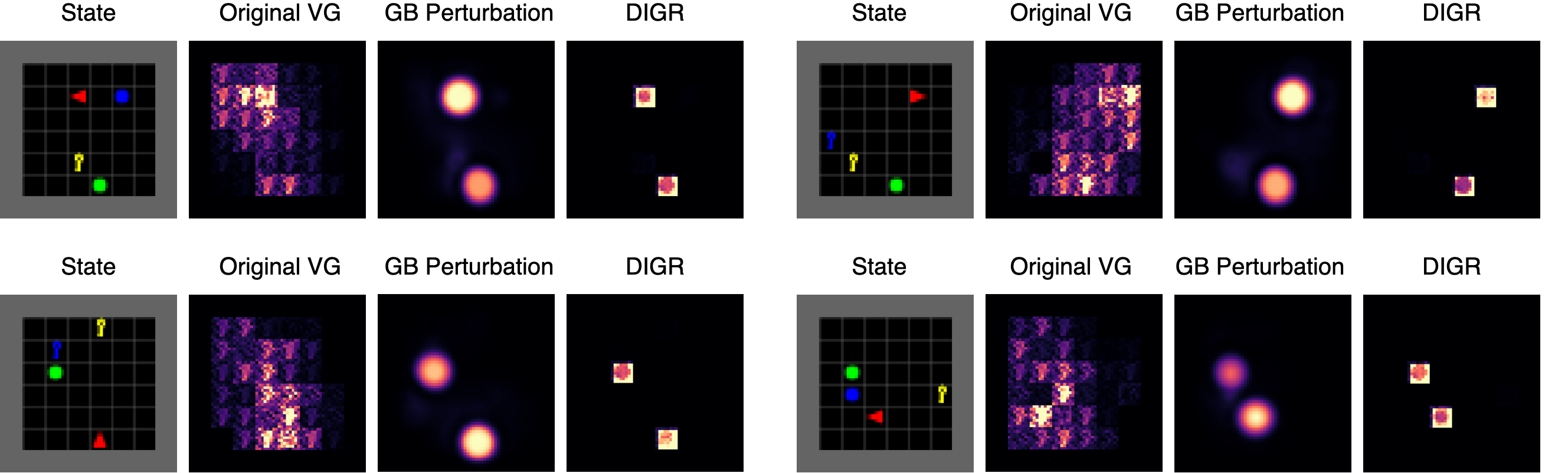
The main goal of our approach is allowing RL policies to generate interpretable saliency maps with computationally efficient gradient-based methods. To demonstrate the effectiveness of our approach, we provide examples of the most computationally-efficient Vanilla Gradient saliency maps before and after our method, and Gaussian-Blur perturbation saliency maps that work as supervisory guidance in Figure 3, 4 and 5.
Our results show that Vanilla Gradient saliency maps generated by original RL policies are noisy and hard to interpret. However, after the optimization with our approach, we can use the same saliency map method to generate much more interpretable saliency maps which reduces a large amount of unexplainable saliency and demonstrate high saliency on task-relevant features only. The saliency maps generated by our approach also have a close similarity to Gaussian-Blur perturbation-based saliency maps which demonstrates the successful saliency guidance. We provide more visual examples containing saliency maps produced by other gradient-based methods for comparison in the appendix.
4.3 Importance of Computational Efficiency
In this section, we further show the importance our approach by demonstrating that missing either computation efficiency or high interpretability make it difficult to achieve interpretable RL in real-world scenarios. We take Autonomous Driving as an example and show the results of utilizing different saliency maps to explain a sequence of RL decision making in Figure 6. In our experiments, the state of CARLA Autonomous Driving is a 128x128 RGB image taken every 0.05 seconds by a camera attached to the ego vehicle. Although Gaussian-Blur perturbation-based saliency maps show high interpretability as seen in Figure 5, it takes 0.97±0.02 seconds to generate one saliency map with a GPU of RTX 2080Ti. This means there’s a delay of almost one second between meeting the state and the availability of corresponding saliency map and all saliency maps for states experienced during the delay will be missed. In constrast to Gaussian-Blur perturbation-based saliency maps that each takes 0.97 seconds to generate in average, Vanilla Gradient saliency maps are much more efficient to compute and take only 0.0021±0.0001 seconds for each state with the same machine. However, Vanilla Gradient saliency maps generated by normal RL policies are hard to interpret and only our approach achieves both computation efficiency and high interpretability.

4.4 Saliency Dataset and Evaluation
Besides illustrative examples, we also aim to provide a quantitative evaluation of saliency maps generated by different approaches and thus introduce a new saliency dataset based on Red-Fetch-Green. Different from previous work that relies on expert annotations and classifies each state element as either important or unimportant feature (Puri et al., 2020), we focus on features whose saliency importance are certain. There are six types of objects in Red-Fetch-Green including the red agent, the green target object, the blue and yellow distrators, grey walls and black empty grids. Based on the roles of objects, we assume the red agent and green target are important features as they have the most important information required for optimal decision making and assume the empty tiles as unimportant features since they do not provide any information. The two distractors and grey walls are not included in the dataset because their influence on decision making is either uncertain or only exists in a small subset of state space. We collected 10k states in the saliency dataset and provide an example in Figure 7.


| Saliency on Red-Fetch-Green | |||
|---|---|---|---|
| important | unimportant | AUC | |
| VG | 56.04 | 278.10 | 0.840 |
| Guided BP | 82.84 | 35.67 | 0.993 |
| Grad-CAM | 43.12 | 364.97 | 0.686 |
| Smooth G | 83.05 | 84.76 | 0.991 |
| Integrated G | 67.79 | 232.09 | 0.900 |
| GB Perturbation | 86.11 | 77.81 | 0.989 |
| SARFA | 58.40 | 42.17 | 0.895 |
| DIGR | 72.52 | 0.00 | 0.997 |

To evaluate the quality of different saliency maps, we compute the average amount of important saliency and unimportant saliency in each saliency map. Furthermore, we also compare different saliency maps with AUC, which is a popular metric used to evaluate saliency maps (Iyer et al., 2018; Puri et al., 2020). As shown in Table 1, our approach keeps a comparable amount of important saliency, reduces all unimportant saliency and achieves the highest AUC compared with other approaches. The decreased amount of unimportant saliency is in line with our expectation since our approach works by penalizing the saliency that are not helpful for interpretation. As a result, our approach utilizes gradient-based and perturbation-based saliency maps for training and finally achieves even better saliency maps.
4.5 Policy Performance Maintenance
The objective of optimizing gradient-based saliency maps may change the action selection of the original policy and thus cause the policy performance to degrade. In DIGR, we use policy distillation to constrain the output of the new RL policy to remain close to the original policy. To verify its effectiveness, we plot the performance of DIGR policy during training and compare it with the results of the original policy. As seen in Figure 9, the policy trained with our approach could achieve similar performance as the original policy.

4.6 Improved Robustness to Attacks
Recent research shows a deep entanglement between adversarial attacks and interpretability of deep neural network (DNN) models (Tao et al., 2018; Ignatiev et al., 2019). Since DIGR improves the interpretability of Deep RL policies, we are also interested in its influence on policy’s robustness to attacks. To study that, we evaluate the robustness of RL policies before and after applying DIGR to four types of adversarial attacks including Fast Gradient Sign Method (FGSM) (Huang et al., 2017), Projected Gradient Descent (PGD) (Madry et al., 2018), Momentum Iterative Fast Gradient Sign Method (MI-FGSM) (Dong et al., 2018) and Maximum Action Difference (MAD) (Zhang et al., 2020) in Red-Fetch-Green and CARLA Autonomous Driving tasks. Since both policy distillation and input gradient regularization in our approach could affect the robustness of RL policies, we further include an ablation study by conducting policy distillation only to understand their own influence on robustness. As shown in Figure 8, our approach significantly improves the robustness of RL policies. Although policy distillation also improves the robustness slightly, selective input gradient regularization contributes the most to the significant robustness gains.
5 Conclusion
We propose an approach called DIGR to improve the efficient interpretability of RL by retraining a policy with selective input gradient regularization and policy distillation. Our approach allows RL policies to generate highly interpretable saliency maps with computationally efficient gradient-based methods. We further show that our approach is able to improve the robustness of RL polices to multiple adversarial attacks. Interpretable decision-making and robustness to attacks are two challenges in deploying RL to real-world systems. We believe our approach could help to build trustworthy agents and benefit the deployment of RL policies in practice.
References
- Chevalier-Boisvert et al. (2018) Chevalier-Boisvert, M., Willems, L., and Pal, S. Minimalistic gridworld environment for openai gym. https://github.com/maximecb/gym-minigrid, 2018.
- Czarnecki et al. (2019) Czarnecki, W. M., Pascanu, R., Osindero, S., Jayakumar, S., Swirszcz, G., and Jaderberg, M. Distilling policy distillation. In The 22nd International Conference on Artificial Intelligence and Statistics, pp. 1331–1340. PMLR, 2019.
- Dong et al. (2018) Dong, Y., Liao, F., Pang, T., Su, H., Zhu, J., Hu, X., and Li, J. Boosting adversarial attacks with momentum. In Proceedings of the IEEE conference on computer vision and pattern recognition, pp. 9185–9193, 2018.
- Dosovitskiy et al. (2017) Dosovitskiy, A., Ros, G., Codevilla, F., Lopez, A., and Koltun, V. Carla: An open urban driving simulator. In Conference on robot learning, pp. 1–16. PMLR, 2017.
- Ferdowsi et al. (2018) Ferdowsi, A., Challita, U., Saad, W., and Mandayam, N. B. Robust deep reinforcement learning for security and safety in autonomous vehicle systems. In 2018 21st International Conference on Intelligent Transportation Systems (ITSC), pp. 307–312. IEEE, 2018.
- Fong & Vedaldi (2017) Fong, R. C. and Vedaldi, A. Interpretable explanations of black boxes by meaningful perturbation. In Proceedings of the IEEE International Conference on Computer Vision, pp. 3429–3437, 2017.
- Fujimoto et al. (2018) Fujimoto, S., Hoof, H., and Meger, D. Addressing function approximation error in actor-critic methods. In International Conference on Machine Learning, pp. 1587–1596. PMLR, 2018.
- Greydanus et al. (2018) Greydanus, S., Koul, A., Dodge, J., and Fern, A. Visualizing and understanding atari agents. In International Conference on Machine Learning, pp. 1792–1801. PMLR, 2018.
- Haarnoja et al. (2018) Haarnoja, T., Zhou, A., Abbeel, P., and Levine, S. Soft actor-critic: Off-policy maximum entropy deep reinforcement learning with a stochastic actor. In International Conference on Machine Learning, pp. 1861–1870. PMLR, 2018.
- Huang et al. (2017) Huang, S., Papernot, N., Goodfellow, I., Duan, Y., and Abbeel, P. Adversarial attacks on neural network policies. arXiv preprint arXiv:1702.02284, 2017.
- Ignatiev et al. (2019) Ignatiev, A., Narodytska, N., and Marques-Silva, J. On relating explanations and adversarial examples. In Wallach, H., Larochelle, H., Beygelzimer, A., d'Alché-Buc, F., Fox, E., and Garnett, R. (eds.), Advances in Neural Information Processing Systems, volume 32. Curran Associates, Inc., 2019. URL https://proceedings.neurips.cc/paper/2019/file/7392ea4ca76ad2fb4c9c3b6a5c6e31e3-Paper.pdf.
- Iyer et al. (2018) Iyer, R., Li, Y., Li, H., Lewis, M., Sundar, R., and Sycara, K. Transparency and explanation in deep reinforcement learning neural networks. In Proceedings of the 2018 AAAI/ACM Conference on AI, Ethics, and Society, pp. 144–150, 2018.
- Lillicrap et al. (2015) Lillicrap, T. P., Hunt, J. J., Pritzel, A., Heess, N., Erez, T., Tassa, Y., Silver, D., and Wierstra, D. Continuous control with deep reinforcement learning. arXiv preprint arXiv:1509.02971, 2015.
- Madry et al. (2018) Madry, A., Makelov, A., Schmidt, L., Tsipras, D., and Vladu, A. Towards deep learning models resistant to adversarial attacks. In International Conference on Learning Representations, 2018. URL https://openreview.net/forum?id=rJzIBfZAb.
- Mnih et al. (2015) Mnih, V., Kavukcuoglu, K., Silver, D., Rusu, A. A., Veness, J., Bellemare, M. G., Graves, A., Riedmiller, M., Fidjeland, A. K., Ostrovski, G., et al. Human-level control through deep reinforcement learning. nature, 518(7540):529–533, 2015.
- Puri et al. (2020) Puri, N., Verma, S., Gupta, P., Kayastha, D., Deshmukh, S., Krishnamurthy, B., and Singh, S. Explain your move: Understanding agent actions using specific and relevant feature attribution. In International Conference on Learning Representations, 2020. URL https://openreview.net/forum?id=SJgzLkBKPB.
- Ross & Doshi-Velez (2018) Ross, A. and Doshi-Velez, F. Improving the adversarial robustness and interpretability of deep neural networks by regularizing their input gradients. In Proceedings of the AAAI Conference on Artificial Intelligence, volume 32, 2018.
- Rosynski et al. (2020) Rosynski, M., Kirchner, F., and Valdenegro-Toro, M. Are gradient-based saliency maps useful in deep reinforcement learning? In ”I Can’t Believe It’s Not Better!” NeurIPS 2020 workshop, 2020. URL https://openreview.net/forum?id=ZF4KyC2zz6x.
- Rusu et al. (2015) Rusu, A. A., Colmenarejo, S. G., Gulcehre, C., Desjardins, G., Kirkpatrick, J., Pascanu, R., Mnih, V., Kavukcuoglu, K., and Hadsell, R. Policy distillation. arXiv preprint arXiv:1511.06295, 2015.
- Schulman et al. (2017) Schulman, J., Wolski, F., Dhariwal, P., Radford, A., and Klimov, O. Proximal policy optimization algorithms. arXiv preprint arXiv:1707.06347, 2017.
- Selvaraju et al. (2017) Selvaraju, R. R., Cogswell, M., Das, A., Vedantam, R., Parikh, D., and Batra, D. Grad-cam: Visual explanations from deep networks via gradient-based localization. In Proceedings of the IEEE international conference on computer vision, pp. 618–626, 2017.
- Silver et al. (2016) Silver, D., Huang, A., Maddison, C. J., Guez, A., Sifre, L., Van Den Driessche, G., Schrittwieser, J., Antonoglou, I., Panneershelvam, V., Lanctot, M., et al. Mastering the game of go with deep neural networks and tree search. nature, 529(7587):484–489, 2016.
- Simonyan et al. (2013) Simonyan, K., Vedaldi, A., and Zisserman, A. Deep inside convolutional networks: Visualising image classification models and saliency maps. arXiv preprint arXiv:1312.6034, 2013.
- Smilkov et al. (2017) Smilkov, D., Thorat, N., Kim, B., Viégas, F., and Wattenberg, M. Smoothgrad: removing noise by adding noise. arXiv preprint arXiv:1706.03825, 2017.
- Springenberg et al. (2014) Springenberg, J. T., Dosovitskiy, A., Brox, T., and Riedmiller, M. Striving for simplicity: The all convolutional net. arXiv preprint arXiv:1412.6806, 2014.
- Sundararajan et al. (2017) Sundararajan, M., Taly, A., and Yan, Q. Axiomatic attribution for deep networks. In International Conference on Machine Learning, pp. 3319–3328. PMLR, 2017.
- Tao et al. (2018) Tao, G., Ma, S., Liu, Y., and Zhang, X. Attacks meet interpretability: Attribute-steered detection of adversarial samples. In Bengio, S., Wallach, H., Larochelle, H., Grauman, K., Cesa-Bianchi, N., and Garnett, R. (eds.), Advances in Neural Information Processing Systems, volume 31. Curran Associates, Inc., 2018. URL https://proceedings.neurips.cc/paper/2018/file/b994697479c5716eda77e8e9713e5f0f-Paper.pdf.
- Vinyals et al. (2019) Vinyals, O., Babuschkin, I., Czarnecki, W. M., Mathieu, M., Dudzik, A., Chung, J., Choi, D. H., Powell, R., Ewalds, T., Georgiev, P., et al. Grandmaster level in starcraft ii using multi-agent reinforcement learning. Nature, 575(7782):350–354, 2019.
- Wang et al. (2016) Wang, Z., Schaul, T., Hessel, M., Hasselt, H., Lanctot, M., and Freitas, N. Dueling network architectures for deep reinforcement learning. In International conference on machine learning, pp. 1995–2003. PMLR, 2016.
- Yu et al. (2020) Yu, T., Kumar, S., Gupta, A., Levine, S., Hausman, K., and Finn, C. Gradient surgery for multi-task learning. In Larochelle, H., Ranzato, M., Hadsell, R., Balcan, M. F., and Lin, H. (eds.), Advances in Neural Information Processing Systems, volume 33, pp. 5824–5836. Curran Associates, Inc., 2020. URL https://proceedings.neurips.cc/paper/2020/file/3fe78a8acf5fda99de95303940a2420c-Paper.pdf.
- Zhang et al. (2020) Zhang, H., Chen, H., Xiao, C., Li, B., Liu, M., Boning, D., and Hsieh, C.-J. Robust deep reinforcement learning against adversarial perturbations on state observations. In Larochelle, H., Ranzato, M., Hadsell, R., Balcan, M. F., and Lin, H. (eds.), Advances in Neural Information Processing Systems, volume 33, pp. 21024–21037. Curran Associates, Inc., 2020. URL https://proceedings.neurips.cc/paper/2020/file/f0eb6568ea114ba6e293f903c34d7488-Paper.pdf.
- Zhang et al. (2018) Zhang, J., Bargal, S. A., Lin, Z., Brandt, J., Shen, X., and Sclaroff, S. Top-down neural attention by excitation backprop. International Journal of Computer Vision, 126(10):1084–1102, 2018.
Appendix A Experiment details and hyperparameters
We conduct experiments on three tasks including Red-Fetch-Green in MiniGrid, Breakout in Atari games and CARLA Autonomous Driving to demonstrate the effectiveness of our approach. To generate the trained reinforcement learning (RL) policies, we use Proximal Policy Optimization (PPO) as the trianing algorithm and list hyperparameters in Table 2.
| Hyperparameters | Red-Fetch-Green | Breakout | CARLA Driving |
| 0.99 | 0.99 | 0.999 | |
| 0.95 | 0.95 | 0.95 | |
| entropy bonus coefficient | 0.01 | 0.01 | 0.01 |
| value loss coefficient | 0.5 | 0.5 | 0.5 |
| gradient clipping | 0.5 | 0.5 | 0.5 |
| PPO clip range | 0.2 | 0.2 | 0.2 |
| learning rate | 0.001 | 0.0002 | 0.0002 |
| total timesteps | 10M | 20M | 1M |
| # environments | 16 | 8 | 1 |
| # timesteps per rollout | 128 | 128 | 1000 |
| # epochs per rollout | 4 | 4 | 4 |
| # minibatches per rollout | 8 | 4 | 4 |
| frame stack | 1 | 2 | 1 |
When applying our approach, we need to choose the saliency threshold to select saliency that will be penalized, weighting parameter to balance selective input gradient regularization and policy distillation, learning rate and online state buffer size. Furthermore, in practice, since we use conduct input gradient regularization based on perturbation-based saliency maps collected in advance instead of producing them from the state buffer, we also need to choose the number of perturbation-based saliency maps in the offline perturbation saliency dataset. We list these hyperparameters in Table 3.
| Hyperparameters | Red-Fetch-Green | Breakout | CARLA Driving |
|---|---|---|---|
| saliency threshold | 0.1 | 0.1 | 0.1 |
| weighting parameter | 0.01 | 0.01 | 1 |
| learning rate | 0.001 | 0.001 | 0.0002 |
| optimizer | Adam | Adam | RMSprop |
| online state buffer size | 10K | 10K | 10K |
| # perturnation-based saliency maps | 1K | 10K | 2.5K |
In this work, we use multiple saliency map methods including Vanilla Gradient, Guided Backpropagation, Grad-CAM, Integrated Gradient, Smooth Gradient, Guassian-Blur Perturbation and SARFA. For Grad-CAM, we report the saliency maps extracted from the last convolutional layer. For Integrated Gradient method, we use 50 interpolation steps to calculate the saliency maps. In our experiments, Smooth Gradient saliency maps are produced by applying SmoothGrad on Guided Backprop saliency maps. For SmoothGrad, we set the noise scale as 0.15 and the number of samples as 20. One important hyperparameter in Gassuain-Blur perturbation-based method is the radius size of the perturbation. Based on the size of the state images and features, we set radius as 4, 8, 5 in Red-Fetch-Green, Breakout and CARLA Autonomous Driving. SARFA is based on Gassuain-Blur perturbation and thus share the same hyperparameters.
Appendix B Additional Experiment Results
In this section, we provide more examples to demonstrate the effectiveness of DIGR. Besides Vanilla Gradient and Gaussian-Blur perturbation-based saliency maps, we also provide Guided Backprop, Grad-CAM, Integrated Gradient and Smooth Gradient saliency maps for comparison. All these saliency maps except DIGR are produced by the policy trained with PPO algorithm. The results on Red-Fecth-Green, Breakout and CARLA Autonomous Driving are shown in Figure 10, 11 and 12.


