POLARIZATION SPECTRUM OF NEAR INFRARED ZODIACAL LIGHT
OBSERVED WITH CIBER
Abstract
We report the first measurement of the zodiacal light (ZL) polarization spectrum in the near-infrared between 0.8 and 1.8 m. Using the low-resolution spectrometer (LRS) on board the Cosmic Infrared Background Experiment (CIBER), calibrated for absolute spectrophotometry and spectropolarimetry, we acquire long-slit polarization spectral images of the total diffuse sky brightness towards five fields. To extract the ZL spectrum, we subtract contribution of other diffuse radiation, such as the diffuse galactic light (DGL), the integrated star light (ISL), and the extragalactic background light (EBL). The measured ZL polarization spectrum shows little wavelength dependence in the near-infrared and the degree of polarization clearly varies as a function of the ecliptic coordinates and solar elongation. Among the observed fields, the North Ecliptic Pole shows the maximum degree of polarization of 20, which is consistent with an earlier observation from the Diffuse Infrared Background Experiment (DIRBE) aboard on the Cosmic Background Explorer (COBE). The measured degree of polarization and its solar elongation dependence are reproduced by the empirical scattering model in the visible band and also by the Mie scattering model for large absorptive particles, while the Rayleigh scattering model is ruled out. All of our results suggest that the interplanetary dust is dominated by large particles.
1 Introduction
The zodiacal light (ZL) arises from sunlight scattered by the interplanetary dust (IPD) in the optical and the near-infrared , and from thermal emission from IPD in the mid- and far-infrared . Measuring the ZL is important for understanding the structure of the IPD distribution and physical properties of the IPD, such as their size distribution, composition, shape, and complex refractive index. In addition, information obtained from ZL measurements is important for future studies of dust disks of exoplanetary systems. . Because the IPD grains of these sizes fall into the Sun , IPD dating to the early solar system is unlikely to exist today. A continuous supply of IPD particles is necessary to maintain the zodiacal cloud.
The source of the IPD is assumed to comprise both comets and asteroids, but the relative importance of each has not been settled. Nesvorný et al. (2010, 2011) compared their dynamical simulations of the IPD with the Infrared Astronomical Satellite (IRAS) data suggesting that 85 of the observed mid-infrared emission is produced by particles from Jupiter-family comets (JFCs) and by dust from long-period comets. Fernández et al. (2006) showed that the geometric albedo of comet 162P/Siding Spring (P/2004 TU12), which is largest radii among known JFCs, is in H band, in R band, and in V band. Soderblom et al. (2002) also observed the JFC 19P/Borrelly and derived a geometric albedo of . The IPD is also known to be a low albedo (Kelsall et al., 1998) and has similarities to the comet nucleus. Yang & Ishiguro (2015) derived the spectral gradient of IPDs as nm at 460 nm, and combining with the albedo showed that of the IPDs originate from comets or D-type asteroids. The ZL spectra measured by the Near Infrared Spectrometer (NIRS) on board the Infrared Telescope in Space (IRTS) and the Cosmic Infrared Background Experiment (CIBER) show silicate-like features at 0.9 and 1.6 m (Matsumoto et al., 1996; Tsumura et al., 2010), comparable to fresh and active comets or S-type asteroids. A combination of amorphous and crystalline silicate grain features is found in ZL spectrum between 9 and 11m (Ootsubo et al., 1998; Reach et al., 2003; Ootsubo et al., 2009).
The ZL scattered by an optically thin cloud of IPDs presents a systematic polarization. The linear polarization degree of sunlight scattered by IPD surfaces is usually defined as the difference between the intensities polarized along the planes perpendicular, , and parallel, , to the scattering plane:
According to Kelsall et al. (1998), the ZL intensity observed at wavelength as the integral along the line of sight is expressed as:
where is the three-dimensional density of the IPD, is the albedo at wavelength , is the solar flux, and is the phase function at scattering angle . Since the polarization properties of scattered light depend on the scattering angle and the composition of the IPD, the origin of the IPD can be investigated by the polarization spectrum of ZL at various fields. For example, the cometary dust ejected from comets is studied by polarization measurements. Zubko et al. (2014) studied dust in comet C/1975 V1 (West) and reproduced the polarization measurement by models with Mg-rich silicate and amorphous carbon. Lasue et al. (2009) also studied dust of comet C/1995 O1 Hale-Bopp and 1P/Halley based on the polarization measurement and implied that the cometary dust can be explained by mixture of a non-absorbing silicate-type material and a more absorbing organic-type material.
A few studies report polarization measurements of the ZL. Leinert et al. (1998) summarized the ZL polarization measured from space in the visible and the near-infrared, and the degree of polarization is largely dependent on the helio-ecliptic longitude to first order. At visible wavelengths, and shows little wavelength dependence (Weinberg & Hahn, 1980; Pitz et al., 1979; Leinert & Blanck, 1982). In the near-infrared, only Berriman et al. (1994) has measured the polarization of the ZL from space by the Diffuse Infrared Background Experiment (DIRBE) aboard on the Cosmic Background Explorer (COBE) in discrete photometric bands at 1.25, 2.2, and 3.5 m. This result shows that the degree of polarization of the ZL is about 10 at solar elongation = 90∘.
In this paper, we report a ZL polarization spectrum measurement from the Low Resolution Spectrometer (LRS) onboard CIBER. The purpose of polarization observation by LRS was to separate polarized ZL from unpolarized EBL, and to identify spectral features by studying the wavelength dependence of polarization. Our result is the first measurement of the ZL polarization spectrum in the near-infrared.
2 LOW RESOLUTION SPECTROMETER/CIBER
| Exposure | Payload’s | Ecliptic | Galactic | Equatorial | Solar Elong. | ZL model | |
|---|---|---|---|---|---|---|---|
| Field Name | Time | Altitude | (, ) | (, ) | (, ) | ||
| (s) | (km) | (deg) | (deg) | (deg) | (degree) | (nW m-2 sr-1) | |
| Lockman Hole | 47 | 202-265 | (135.42, 45.49) | (149.41, 51.97) | (161.43, 58.21) | 118.8 | 330.23 |
| SWIRE/ELAIS-N1 | 45 | 284-315 | (209.32, 72.32) | (84.31, 44.71) | (242.81, 54.59) | 105.7 | 269.12 |
| North Ecliptic Pole (NEP) | 53 | 320-324 | (311.48, 89.62) | (96.06, 29.56) | (270.63, 66.28) | 90.0 | 280.55 |
| Elat30 ( = 30 degree) | 26 | 319-306 | (234.38, 29.25) | (18.64, 44.89) | (236.98, 9.57) | 124.1 | 403.53 |
| BOOTES-B | 50 | 296-244 | (200.35, 44.82) | (55.13, 68.06) | (217.30, 33.27) | 132.3 | 328.47 |
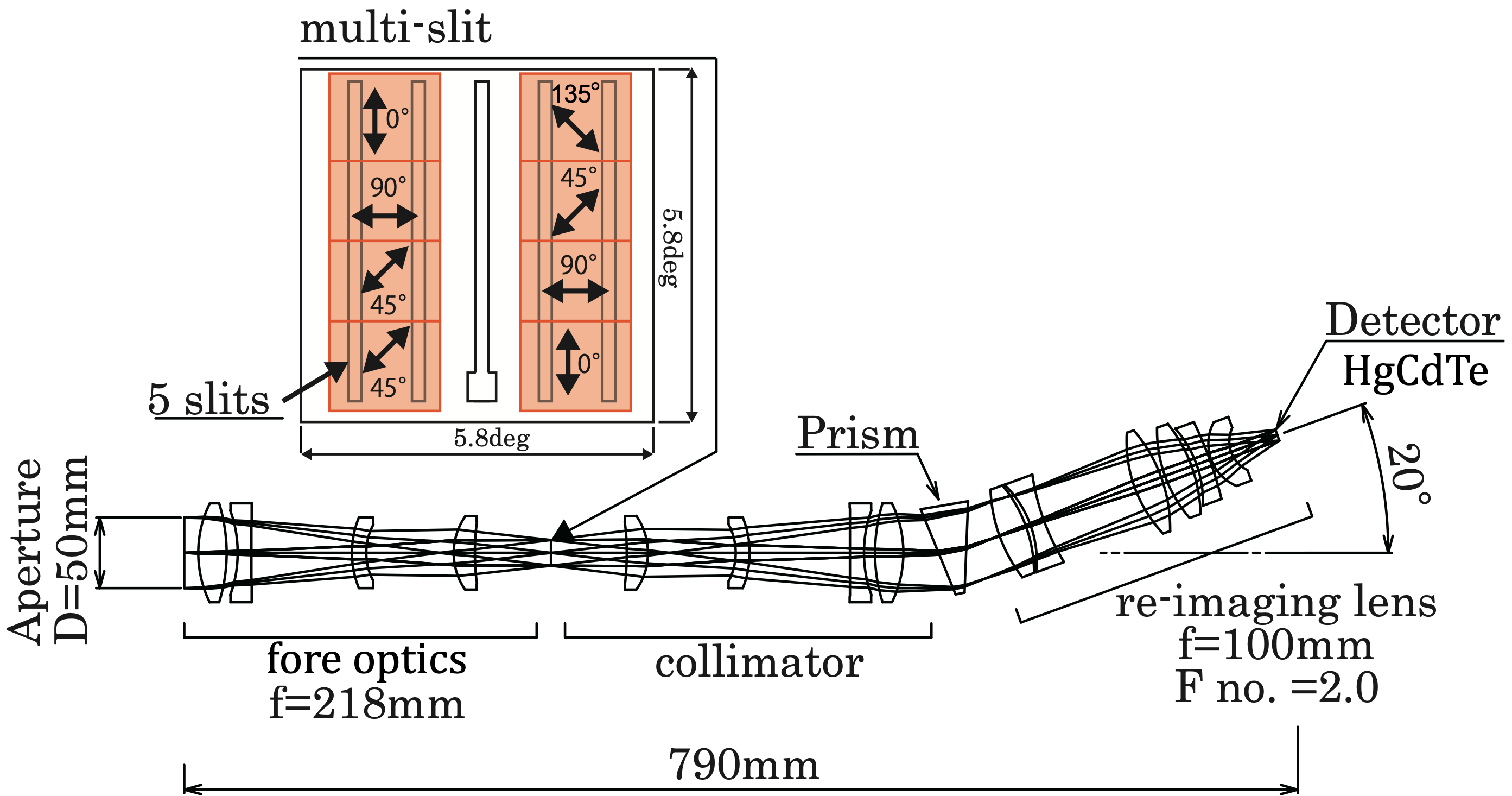
CIBER, designed to study the diffuse near-infrared emission above the Earth’s atmosphere (Zemcov et al., 2013), housed three instruments including a two broad-band imagers (Bock et al., 2013), a narrow band spectrometer (Korngut et al., 2013), as well as the LRS designed to measure the spectrum of diffuse light in 0.8 1.8 m (Tsumura et al., 2013) with a wavelength resolution of -30. Fore optics of the LRS brings an image of the sky to focus on a mask containing 5 slits as shown in Figure 1, each spanning a field of view (FOV) of 52.7′ sampled by a 256256 pixel HgCdTe array. This array hosts a cold shutter assembly for dark current measurement.
CIBER conducted observations four times, on February 2009, July 2010, March 2012, and June 2013. The payload was successfully recovered and refurbished after the first three flights. Because the polarizers were only installed in the third flight, we mainly use the third flight data in this paper. At the third flight, we used NASA Black Brant IX111For details on the launch vehicles, Sounding rocket handbook (http://sites.wff.nasa.gov/code810/files/SRHB.pdf). two-stage vechicles launched from the White Sands Missile Range in New Mexico, USA. The apogee on the flight was 330km, providing a total exposure time of 240 seconds. The raw data, which are non-destructively sampled by the integrating detectors, were telemetered to the ground from the rocket during the flight. The celestial attitude control system achieved a pointing stability of 8′′. Details about the CIBER payload and flight performance are written in Zemcov et al. (2013). See Tsumura et al. (2013) and Arai et al. (2015) for details of the LRS.
To measure the polarization spectrum, we installed wire-grid polarization film 222Manufactured by Asahikasei E-materials corporation. on the slit mask. The wire-grid polarization films with different transmittance axis were installed on eight different regions of the slit mask (Figure 1). Although the FOV of each polarizer is different, the ZL is smoothly distributed over the entire FOV and small field-to-field fluctuations if any can be corrected for. Therefore, if the integrated star light (ISL) and diffuse galactic light (DGL) can be removed, ZL polarization can be measured with this instrument.
The phase angles of the transmittance axis of the polarizer are labeled as = (Figure 1). Note that the polarizing film in the lower left corner was mistakenly installed with the transmission axis rotated by 90 degrees during the final installation, but it was calibrated and launched as it was. Because the polarizing films were not installed on the center slit, the total spectrum of the sky brightness was also measured.
The observed fields are listed in Table 1. For the ZL analysis, the fields are selected based on ecliptic coordinates and solar elongation. The low ecliptic latitude field, Elat30, shows high ZL brightness. On the other hand, the high ecliptic latitude fields exhibit low ZL brightness. The North Ecliptic Pole (NEP) field, where the solar elongation is 90∘, is selected because the polarization is expected to be maximum. As the solar elongation increases, the polarization is expected to decrease.
3 INSTRUMENTAL CALIBRATION FOR POLARIMETRY
We describe the wavelength calibration, surface brightness calibration, and flat field correction, and polarization calibration in this section. The wavelength calibration, surface brightness calibration, and flat field correction are similar to Arai et al. (2015).
3.1 Wavelength Calibration
We conduct the wavelength calibration, which measures the relationship between the incident monochromatic light and a position on the detector array. For spectral calibration in the laboratory, we use two different light sources consisting of the SIRCUS (spectral irradiance and radiance responsivity calibrations using uniform sources) laser facility and a standard quartz-tungsten-halogen lamp coupled to a monochrometer. To illuminate the LRS, both light sources are coupled via fiber to an integrating sphere 20 cm in diameter. After exposure to a monochromatic light source, the detected signal is fitted with a Gaussian function. The accuracy of the wavelength calibration is calculated to be 1 nm by combining the center of this Gaussian function with the externally determined wavelength of the incident light.
3.2 Surface Brightness Calibration
The LRS sensitivity requirement is , corresponding to 4% level of the sky brightness. To find the conversion between the photocurrent and the surface brightness, we use two different light sources consisting of the SIRCUS laser facility and a super-continuum laser (SCL). Both light sources coupled to a 20 cm diameter integrating sphere through a fiber illuminating the LRS aperture. The calibration factor is calculated from the measurement results of both light sources. The statistical uncertainty of 1 is estimated to be less than 0.1% from the variance over all pixels of the detector array. The measured calibration factor is consistent within a 3 r.m.s variation.
3.3 Flat Field Correction
In order to correct for the spatial fluctuations generated by the detector’s nonuniform response, we use laboratory measurements to construct the flat field. We use three different light sources consisting of the SIRCUS laser facility, SCL, and a standard quartz-tungsten-halogen lamp with a solar-like filter. All light sources are coupled via fiber to an integrating sphere with a diameter of 10 or 20 cm, which then illuminates the aperture of the LRS. By combining various light sources and integrating spheres, we can quantify the systematic uncertainty of the flat field correction. The illumination patterns of the spheres are uniform with an accuracy of less than 1%.
3.4 Polarization Calibration
In order to characterize the polarization measurement, we conduct the polarization calibration in the laboratory. This polarization calibration determined the transmittance, the extinction ratio, and the relative angle of the LRS polarizer in the laboratory. The extinction ratio quantifies the performance of the polarizer and is expressed as
| (1) |
where is the polarization degree of the light passing through the polarizer, and is the degree of the unpolarization . The extinction ratio of the polarizer for parallel light was known as 1000 in advance, but not for convergent light. The LRS polarizer operates with converging rays, so its extinction ratio needs to be measured in the laboratory before the flight.
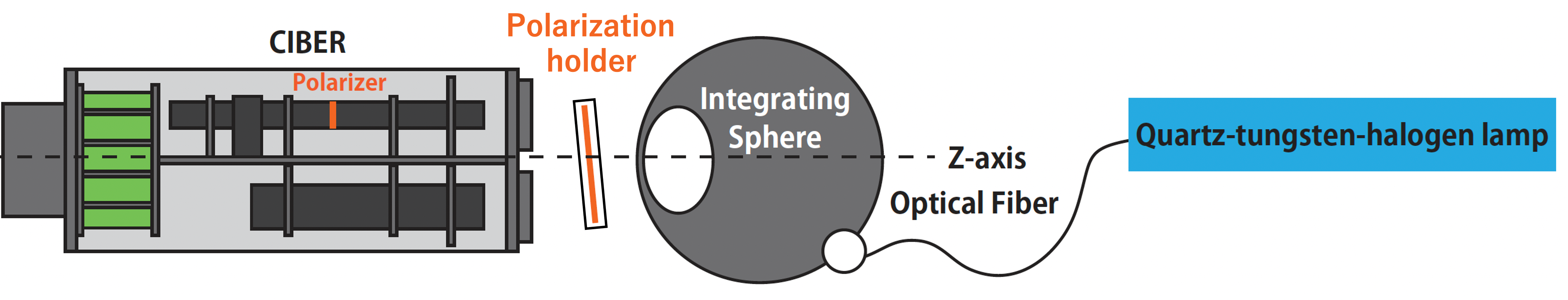
A schematic view of the setup for the polarization calibration is shown in Figure 2. A standard quartz-tungsten-halogen lamp is used as light source and is coupled to an integrating sphere through a fiber illuminating the LRS aperture. A 100 mm diameter wire-grid polarizing film is settled between the LRS aperture and the integrating sphere, which is installed on a rotational polarization holder. The polarization holder is rotated around the optical axis of the LRS by 10∘ step.
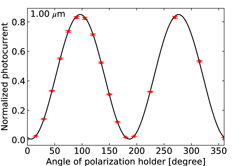
In Figure 3, we show the normalized photocurrent measured with the LRS as a function of the angle of the polarization holder . To quantify the degree of polarization and the extinction ratio, we fit the following equation with the Levenberg-Marquardt algorithm,
| (2) |
where is the brightness of the polarized component, indicates the mean brightness of the light source, and represents the phase angle of polarization. The degree of polarization, is calculated by the following equation,
| (3) |
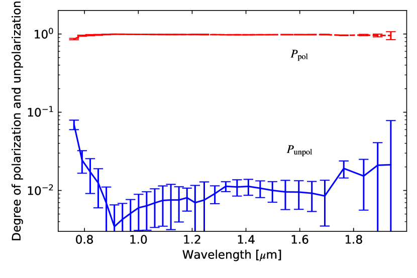
We show the and in Figure 4. Although the for parallel light was larger than 0.999, and is then less than 0.001, measured in the experiment is 0.99. It is due to the oblique incident light at the position where the polarization film is installed in the LRS. However, is acceptably small to measure the polarization of ZL and we regard the unpolarized component of 0.01 offset as a systematic uncertainty in the LRS data.
4 BASIC DATA REDUCTION
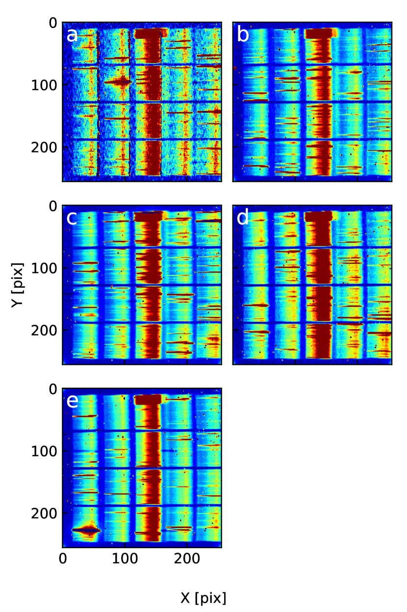
At first, we make the LRS image from individual time-ordered array readout frames. In Figure 5, we give examples of the LRS images in the third flight. The five vertical sections correspond to the five slits dispersed in the direction, and the four parallel sections correspond to the wire-grid polarizing films.
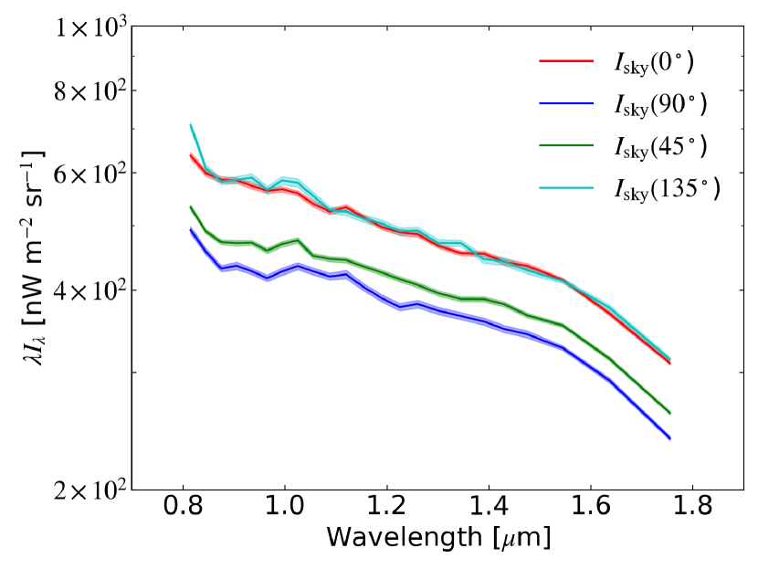
In order to measure the absolute spectrum of the sky brightness, we subtract the dark current and mask bright point sources from the LRS images. The dark current is estimated from the masked regions of each slit individually. The corners of the array are masked to avoid contamination by spurious signals emanating from the multiplexers of the detectors in the corners of each quadrant. To remove bright point sources, we average the photocurrent of each slit along the horizontal direction, then clip the pixels containing stars determined by the criterion that the band-averaged photocurrent is deviated from the mean of band-average photocurrent of all pixels by 2 , where is the standard deviation of the photocurrent. We iterate this clipping procedure until the ratio of the number of rejected pixels to the remaining pixels is less than 0.1 of the total. To reject hot and dead pixels and the remaining faint point sources, pixels which are greater than 3 from the mean are also excluded. Finally, we derive the sky spectrum, , through each polarization filter as shown in Figure 6.
Further details on the basic data reduction are described in Tsumura et al. (2010) and Arai et al. (2015).
5 DATA ANALYSIS
After the basic data reduction, to derive the ZL polarization spectrum, we separate the mean ZL brightness, , and the ZL brightness of the polarized component, , from the measured sky brightness. We assume that the polarization components of the DGL, the ISL, and the EBL are negligible compared to the ZL as discussed in Section 7. The measured sky brightness of the polarized component can then be assumed as .
The mean sky brightness comprises;
| (4) |
To derive , the DGL, the ISL, and the EBL contributions need to be separated from the measured sky brightness (Matsuura et al., 2017). The DGL component, , is derived using its spatial distribution as traced by 100 m emission on scales smaller than a degree (Arai et al., 2015). The ISL component, , is estimated by Monte-Carlo simulation of the star distribution in the FOV using the 2MASS catalogue (Skrutskie et al., 2006), taking into account the limiting magnitude and the effective slit efficiency of the LRS (Arai et al., 2015). The EBL component, , can be assumed as identical in all the fields, but with a lot of indeterminacy. To derive the fiducial unpolarimetric spectral shape of ZL, we calculate the difference between two fields,
| (5) |
where and indicate different observation fields. We assume that the EBL component is identical in all the fields, so is canceled in Equation 5. We also estimate the ZL brightness, , at 1.25 m of each field from the DIRBE/COBE-based ZL model (Kelsall et al., 1998), which are summarized in Table 1, and normalize the differences of with at 1.25 m. Because of deep airglow contamination, only the NEP, Elat-30 and BOOTES-B fields are available to derive the fiducial unpolarimetric spectral shape of ZL with polarization slit of the LRS. To improve the signal-to-noise ratio, we use not only the data with polarization slit but also that with center slit at the NEP and Elat-30 fields, and average these results. It is noteworthy that we could not use the data with center slit at the BOOTES-B field because the detector was not functioning properly. The airglow emission likely depends on atmospheric conditions and changes daily. The details of uncertainty of the airglow contamination are described in Section 7.
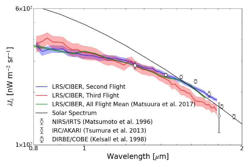
Figure 7 presents the fiducial mean spectral shape of ZL during the third flight. The difference in the ZL spectral shape between the second and third flights may be due to the timing of the observations and the calibration accuracy. In deriving the ZL polarization spectrum, we only use the ZL spectral shape of the third flight in terms of the instrumental systematic uncertainties.
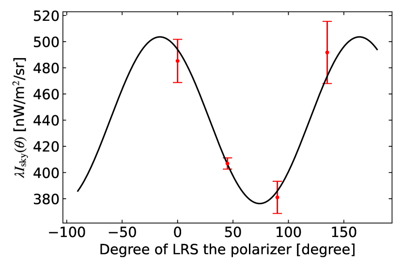
To derive , we fit the measured sky spectrum with Equation 2 to separate the polarized and unpolarized components. In Figure 8, we show the measured at 1.26 m as a function of in the NEP field, as an example of the analysis. The black curve presents best fit by Equation 2.
Finally, from Equation 3, the ZL polarization spectrum can be expressed as,
| (6) |
6 RESULT
6.1 Validity of the Measured Polarization Angle
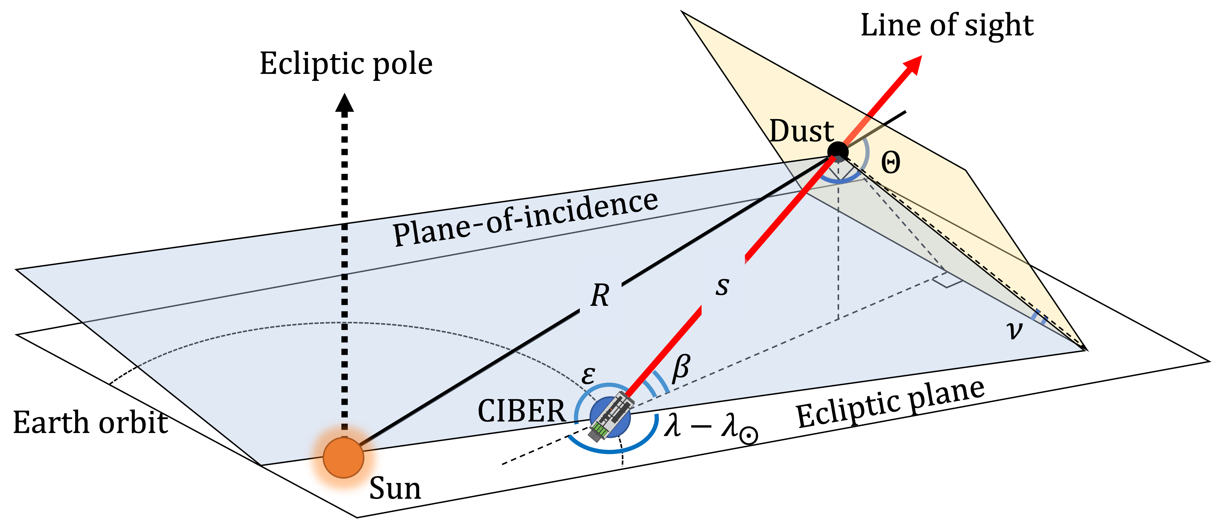
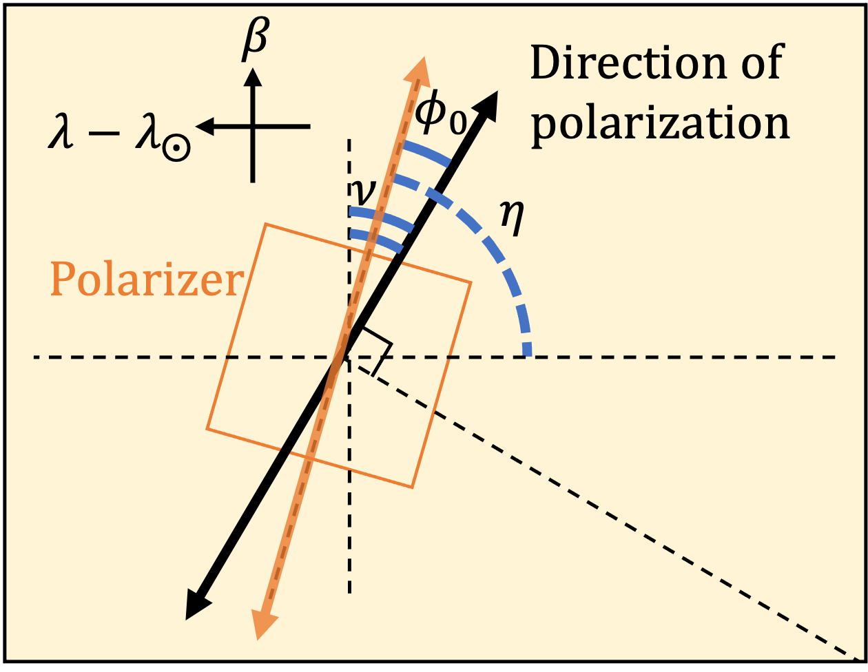
First of all, to validate our measurements, we compare an expected polarization angle, , with the measured polarization angle, . We show the geometric definition of the polarization angle in Figure 9 and 10. The angle of the plane-of-incidence, , toward the declination is presented as
| (7) |
Thus can be determined as
| (8) |
where indicates the rotational angle of the slit. We note that the scattered light by each IPD grain along the line of sight produces the same phase angle since it does not depend on the distance between the LRS and the IPD grains. We summarize these parameters to calculate the expected polarization angle in Table 2. The measured phase angle is generally consistent with expectation, which supports our polarimetric measurements.
| Field Name | (deg) | (deg) | ||||
|---|---|---|---|---|---|---|
| Lockman Hole | 1131 | 11812 | ||||
| SWIRE/ELAIS-N1 | 733 | 684 | ||||
| North Ecliptic Pole (NEP) | 1201 | 1192 | ||||
| Elat30 ( = 30 degree) | 491 | 548 | ||||
| BOOTES-B | 1902 | 1638 |
Note. — Because the LRS has large FOV, is different between the center and the edge of an image. The uncertainty of indicates this difference. is the average over all wavelengths. The uncertainty of represents the standard deviation.
6.2 Polarization Spectra
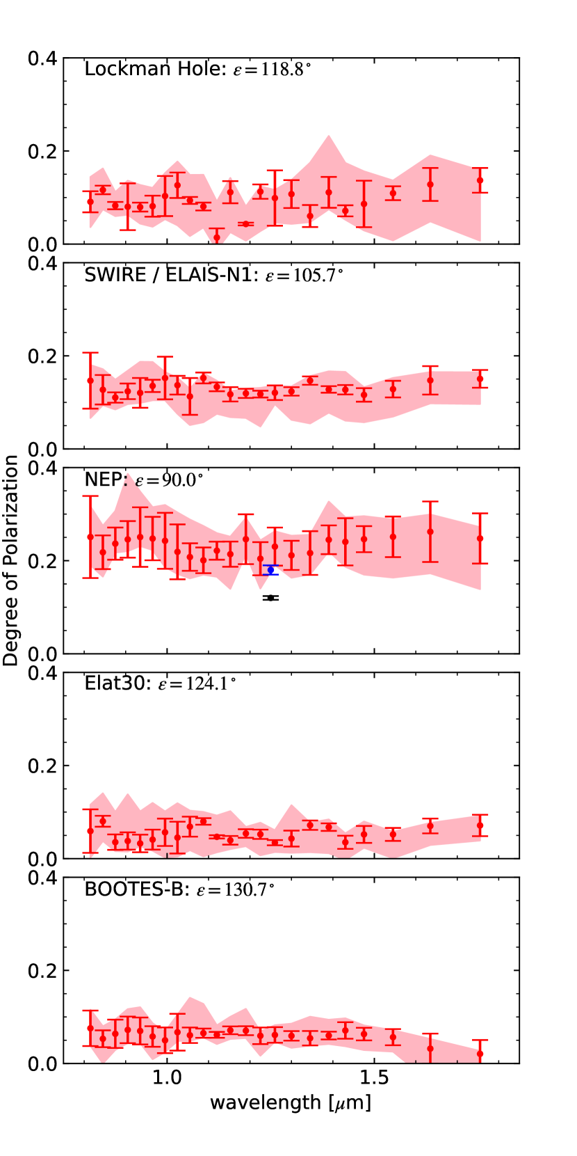
We show the ZL polarization spectrum, , of the five fields measured in the third flight in Figure 11 and Table 3. This is the first measurements of the polarization ZL spectrum in the near-infrared. shows little wavelength dependence in all fields. On the other hand, clearly depends on the ecliptic coordinates and the solar elongation. peaks at the NEP field where the solar elongation is . The detail of systematic uncertainty is described in Section 7.
| (m) | (%) | (%) | (%) | (%) | (%) |
|---|---|---|---|---|---|
| 0.815 | 9.4 2.2 5.3/5.5 | 15.2 6.1 3.4/8.0 | 26.0 8.8 6.6/6.0 | 6.1 4.8 3.4/8.0 | 7.8 3.9 4.0/3.7 |
| 0.845 | 13.1 0.5 4.6/4.2 | 14.3 3.4 4.4/3.3 | 24.5 3.7 5.7/5.2 | 9.0 1.2 4.4/3.3 | 6.0 2.0 2.7/5.3 |
| 0.875 | 8.9 0.6 2.9/2.3 | 11.9 0.9 3.8/2.6 | 25.5 3.3 7.0/1.9 | 3.8 1.8 3.8/2.6 | 6.9 3.2 3.1/3.5 |
| 0.905 | 8.6 5.4 5.6/1.7 | 13.3 1.6 4.4/2.7 | 26.3 3.8 14.1/2.5 | 4.1 2.0 4.4/2.7 | 7.7 3.0 4.5/2.8 |
| 0.935 | 8.4 0.8 4.7/3.5 | 12.7 3.2 6.7/2.2 | 26.4 6.4 9.8/1.9 | 3.4 2.0 6.7/2.2 | 7.4 3.0 5.1/2.6 |
| 0.965 | 8.5 2.3 3.9/4.4 | 14.2 0.9 5.1/3.1 | 25.9 4.5 6.7/2.5 | 4.3 2.2 5.1/3.1 | 6.1 2.3 2.8/4.9 |
| 0.995 | 10.7 4.4 4.9/5.0 | 15.8 4.6 1.3/4.8 | 25.1 5.9 7.7/5.6 | 5.9 3.0 1.3/4.8 | 5.2 2.8 1.8/2.5 |
| 1.025 | 13.0 2.6 5.1/8.6 | 14.1 1.7 1.6/6.1 | 22.5 5.8 8.5/4.7 | 4.7 3.5 1.6/6.1 | 6.9 4.0 3.7/1.9 |
| 1.055 | 9.6 0.4 5.5/7.6 | 11.6 4.0 1.6/6.1 | 21.3 2.7 8.1/4.6 | 7.0 2.2 1.6/6.1 | 6.2 1.7 8.0/1.2 |
| 1.087 | 8.0 0.7 6.8/4.5 | 15.1 0.7 1.0/9.5 | 20.0 2.5 7.4/3.1 | 7.9 0.5 1.0/9.5 | 6.5 0.9 6.3/0.9 |
| 1.120 | 1.4 1.9 7.7/2.6 | 13.1 0.6 1.3/5.8 | 21.8 1.5 3.8/5.6 | 4.6 0.2 1.3/5.8 | 6.1 0.5 2.0/2.0 |
| 1.152 | 10.8 2.2 3.1/8.6 | 11.4 1.3 0.6/4.9 | 20.7 2.3 3.8/7.4 | 3.8 0.9 0.6/4.9 | 6.9 0.7 2.9/1.9 |
| 1.190 | 4.1 0.1 3.8/3.6 | 11.3 0.6 1.0/5.3 | 23.4 4.9 4.5/3.2 | 5.1 0.8 1.0/5.3 | 6.7 0.8 4.7/1.6 |
| 1.225 | 11.4 1.4 1.1/8.5 | 11.9 0.4 1.3/7.0 | 20.7 3.4 3.9/6.4 | 5.3 1.0 1.3/7.0 | 6.0 1.8 0.9/4.3 |
| 1.260 | 9.8 5.9 1.7/5.3 | 12.0 1.4 1.5/2.4 | 22.8 3.9 3.3/3.9 | 3.4 0.5 1.5/2.4 | 6.1 1.6 2.1/1.4 |
| 1.300 | 10.5 2.9 3.0/6.4 | 12.1 0.6 1.1/6.1 | 20.7 2.9 4.2/4.8 | 4.2 1.7 1.1/6.1 | 5.8 1.0 2.6/2.6 |
| 1.345 | 5.9 2.3 11.4/1.3 | 14.3 0.4 1.0/9.2 | 21.1 4.4 3.9/4.6 | 7.0 0.9 1.0/9.2 | 5.3 1.5 4.6/1.6 |
| 1.390 | 10.6 3.1 12.1/3.6 | 12.2 0.3 3.9/5.0 | 23.4 2.7 8.2/2.5 | 6.5 0.7 3.9/5.0 | 5.7 0.8 3.4/1.8 |
| 1.430 | 6.8 1.1 10.3/1.9 | 12.1 0.7 3.8/6.6 | 23.0 4.7 5.3/5.4 | 3.4 1.3 3.8/6.6 | 6.8 1.7 2.6/3.4 |
| 1.475 | 8.0 4.6 7.0/5.7 | 10.8 1.2 1.6/5.9 | 22.9 2.3 4.9/7.6 | 4.8 1.7 1.6/5.9 | 5.9 1.2 1.9/3.4 |
| 1.545 | 10.0 1.3 2.7/10.1 | 11.8 1.5 2.4/5.9 | 23.0 3.8 3.7/8.8 | 4.8 1.2 2.4/5.9 | 5.2 1.6 1.5/3.1 |
| 1.635 | 11.2 3.0 6.2/7.9 | 12.9 2.6 1.8/4.9 | 22.9 5.5 3.7/8.9 | 6.1 1.3 1.8/4.9 | 2.8 2.8 2.1/7.1 |
| 1.755 | 12.2 2.3 2.1/13.0 | 13.4 1.5 1.4/5.4 | 22.1 4.7 2.4/10.9 | 6.4 2.0 1.4/5.4 | 1.9 2.7 0.6/10.3 |
Note. — Mean value Statistical uncertainty Systematic uncertainty (upper/lower).
| Wavelength | Detection | ||||||
|---|---|---|---|---|---|---|---|
| Limit | |||||||
| (m) | () | (Jy) | (nW m-2 sr-1) | (nW m-2 sr-1) | (nW m-2 sr-1) | (nW m-2 sr-1) | () |
| 1.25 | 12.00 0.4 | 15 | 831 41 | 318 15 | 10 1 | 54 17 | 18 1 |
| 2.2 | 10.00 0.5 | 15 | 302 15 | 257 13 | 5 1 | 28 7 | 19 1 |
Note. — See Section 6 for detail.
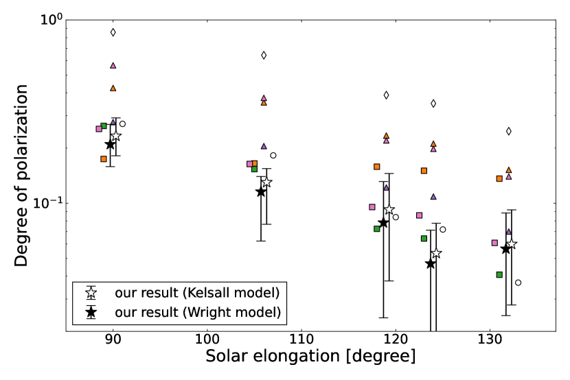
6.3 Solar Elongation Dependence
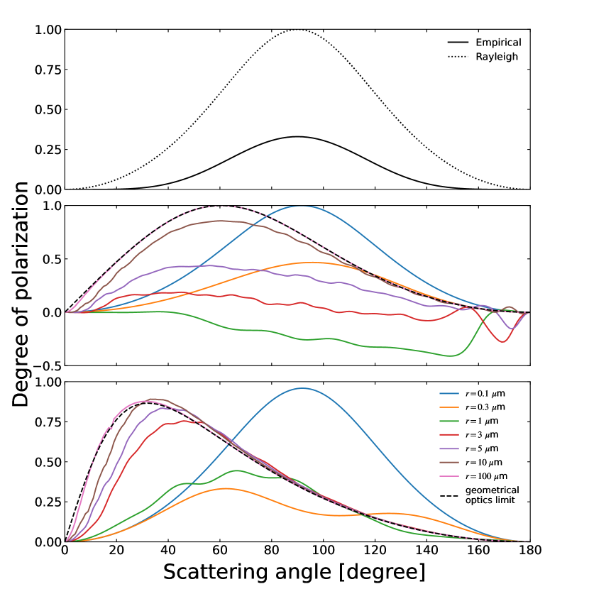
We show the mean of from 0.8 to 1.8 m as a function of the solar elongation in Figure 12. We plot two results scaled to the ZL brightness estimated from the Kelsall et al. (1998) model (hereafter the Kelsall model) and the Wright (1998) model (hereafter the Wright model). The degree of polarization of the IPD as a function of the scattering angle in different scattering models is shown in Figure 13. The models we consider are empirical scattering, Rayleigh scattering, and Mie scattering with astronomical silicate and with graphite (Bohren & Huffman, 1983). For Mie scattering, we assume the mean complex refractive indices for astronomical silicate as typical refractive material and for graphite as a typical absorptive material from 0.8 to 1.8 m (Draine & Lee, 1984). The degree of polarization in each model is calculated by integrating along the line of sight in each field and assuming the IPD geometry of the Kelsall model (Figure 12). Since each observation field in CIBER is toward solar elongation , the degree of polarization with scattering angle is not included in the line-of-sight integration. Our results are consistent with the degree of polarization inferred from the scattering properties of the empirical model and the Mie scattering model with m graphite. The Rayleigh scattering and the Mie scattering with astronomical silicate can be rejected as the principal mechanism of the ZL polarization.
6.4 Comparison with the DIRBE/COBE data
To compare our result with the DIRBE/COBE data at 1.25 and 2.2 m, we estimate the ZL polarization, , from the result presented in Berriman et al. (1994). Because Berriman et al. (1994) did not take into account the DGL, the ISL, and the EBL contributions, they present the polarization of the sky brightness, . In order to estimate , we estimate , , , and . We estimate as the following:
| (9) |
where is estimated from the Kelsall model. is calculated by integrating stars fainter than the detection limit of point sources of DIRBE, at 15 Jy (Arendt et al., 1998). We integrate star light fainter than 15 Jy by using 2MASS catalogue (Skrutskie et al., 2006) and TRILEGAL, which is population synthesis code for Monte-Carlo simulating a star count in the Galaxy (Girardi et al., 2005). The uncertainty of is estimated from the variance due to the Monte-Carlo simulation. is estimated from Arai et al. (2015) and Tsumura et al. (2013a) at 1.25 and 2.2 m. is adopted from Cambrésy et al. (2001). These estimated components are summarized in Table 4. Since these sources can be assumed as unpolarized, we calculate the surface brightness of the polarization component, as
| (10) |
Finally we infer using the estimated and :
| (11) |
The resultant is summarized in Table 4. Although the original DIRBE/COBE data, , indicates redder color than our data, shows little wavelength dependence after we account for other diffuse sources. We show comparison between , , and at the NEP field with the same solar elongation in Figure 11. is consistent with at the NEP field.
7 SYSTEMATIC UNCERTAINTY
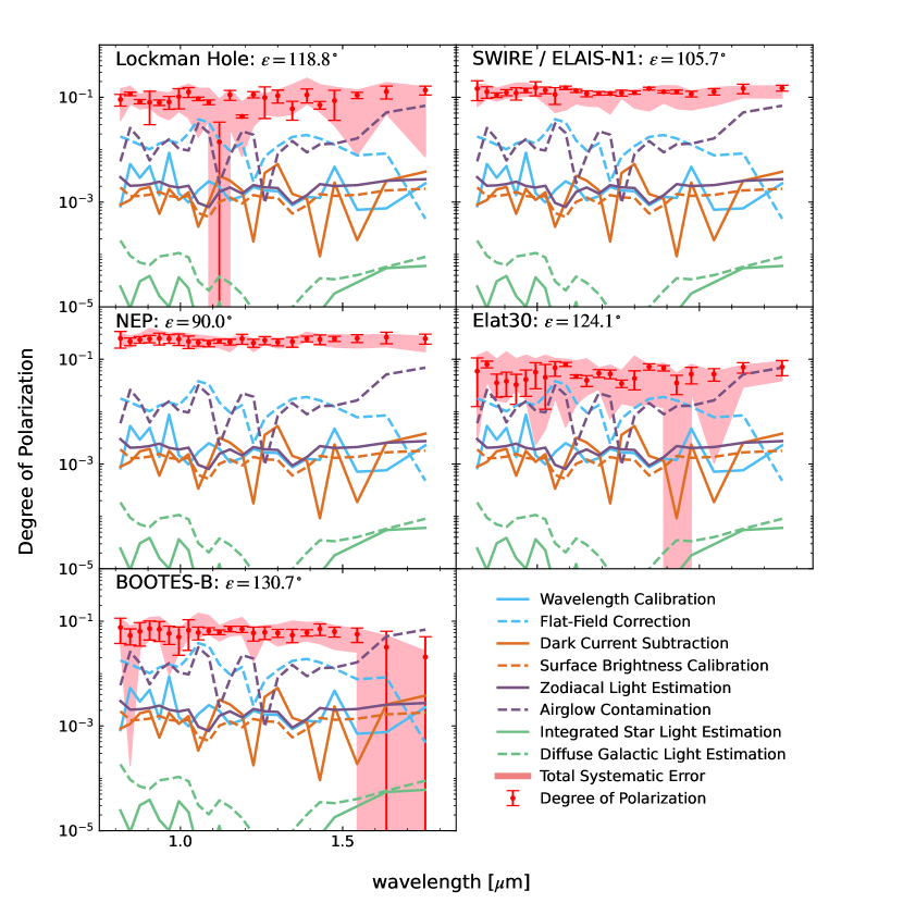
Fig 14 contains the same data as Fig 11, but overplotted with the instrumental and astronomical systematic uncertainties. The systematic uncertainties include the instrumental calibrations, the contributions from airglow emission, and the diffuse brightness estimation. The total systematic uncertainty is the upper limit because we assume maximum polarization of residual faint stars, and the DGL.
7.1 Instrumental Systematic Uncertainty
Since the accuracy of the wavelength calibration is 1 nm, to quantify how the wavelength uncertainty propagates into the ZL polarization spectrum, we shift the wavelength by 1 nm, then recompute the ZL polarization spectrum with the shifted wavelength in each case. The uncertainty due to the wavelength calibration is then captured by the difference between the and shifted ZL spectra. As shown in Figure 14, the propagated uncertainty is negligible.
We estimated the biased introduced by the flat-field correction by differencing the flat-field measurements from various integrating spheres. We used two integrating spheres with 10 cm and 20 cm exit port diameters as described in Arai et al. (2015). We then derive two ZL spectra for these two flat fields, and take their difference as the uncertainty of ZL polarization due to the flat field. The flat-field systematic uncertainty is %, which is acceptably small. To check the systematic uncertainty from the dark current subtraction, we closed a cold shutter and measured the dark current images twice, on the rail and during the flight. The flight-rail difference makes a 0.03 e- s-1 systematic offset corresponding to 0.7 nW m-2 sr-1 at 1.25 m. We subtracted these dark current images from the each sky image and then calculated difference between the rail and flight cases, which gives us the bias from dark current subtraction. The systematic uncertainty in the dark current subtraction does not significantly affect the final results.
In general, the absolute brightness calibration uncertainty is canceled because the calibration is common between the polarization and the brightness channels. However, since we estimate the ZL brightness using a ZL model, a bias arises when comparing our data with the ZL model brightness. As described in Arai et al. (2015), we conduct the absolute brightness calibration with several different setups in the laboratory. The measured calibration factors are consistent to within a 3 r.m.s variation, which sets the uncertainty of the absolute brightness calibration.
To quantify the bias of the polarization measurement, we investigate the LRS polarization calibration data described in Section 3. Although the extinction ratio of the wire-grid polarization film is higher than 1000, the measured extinction ratio of the LRS is 100. The opening angle of incidence at the polarization film in the LRS is large, so some incident light leaks and decreases the extinction ratio of the LRS. This means that the polarization measurement has a 0.01 offset. We regard this offset as the systematic uncertainty of the polarization measurement by the LRS.
7.2 Airglow Contamination
We attribute a time and a rocket-altitude dependence to the airglow emission, so the observed brightness is written as
| (12) |
where indicates the brightness of airglow emission, is the time from the launch, and is the altitude of the rocket. To estimate the contamination from airglow, we separate the sky image into a first and a second-half integrations and derive the ZL polarization spectrum from each half. If there is difference between the ZL polarization spectra derived from the first and the second-half images, this difference should be due to the airglow contamination. We calculate this difference as the bias from the airglow. The measured bias from the airglow contamination is 20 at the Lockman and Elat30 fields, 10 at the BOOTES-B field, 5 at the SWIRE field, and 2 at the NEP field. From these results, we confirm that the airglow contamination decays with time and altitude of the rocket, because the amount of the airglow contamination in the first-half is higher than that in the second half. Because the integration time of Elat30 is shorter than other fields, the large airglow contamination can also be due to noise. As shown in Figure 14, the airglow contamination is not negligible but is acceptably small.
7.3 Astronomical Systematic Uncertainty
Starlight is known to be linearly polarized due to interstellar dust grains aligned by the magnetic field of the Galaxy (Heiles, 2000). The maximum polarization is 0.03 at where is optical depth in V-band (Serkowski, 1973). If the brightness of residual faint stars is 15 of the ZL brightness at the NEP field, the maximum starlight polarization is 0.0045. Because stars are randomly distributed and the LRS FOV is large, the starlight polarization should be lower than this estimation. The starlight polarization is then only a few percent of the ZL polarization, which is negligible.
Because the DGL polarization has never been measured, we adopt the polarization of molecular clouds and reflection nebulae to quantify the DGL polarization. Hashimoto et al. (2007) measured the linear polarization of the Orion molecular clouds and reported that the maximum polarization is 0.10 and 0.19 at J-band and H-band, respectively. Nagata et al. (1987) report that the polarization of the extended reflection nebulae around GGD27 IRS and W75N IRS is 0.2 at 2.2 m. From these results, we assume that the DGL polarization is 0.2. Because the DGL brightness is 10 of the ZL brightness at the NEP field, the contamination by the DGL polarization is 0.02.
8 DISCUSSION
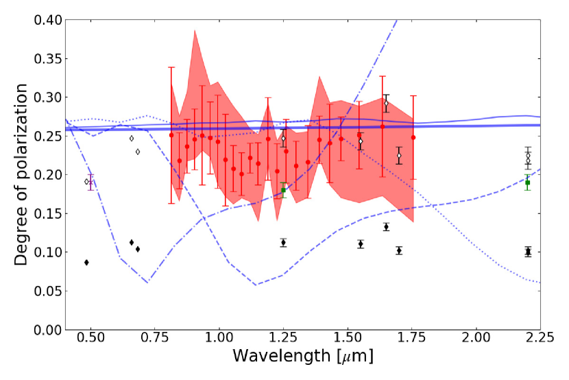
In Figure 15, the ZL polarization has little wavelength dependence from visible to infrared. The similar scattering properties at different wavelengths suggest that large IPD grains contribute to the ZL polarization. This suggestion is supported by the fact that our observations are consistant with the ZL polarization calculated by the empirical scattering model in the visible band. The similar scattering properties at different wavelengths suggest that large IPD grains contribute to the ZL polarization. We provide another test for the IPD size by comparing the ZL polarization spectrum with the polarization of Mie scattering theories. We used five models with different particle radius (=0.3, 0.5, 1, 3, and 10 m) with a constant complex refractive index independent of wavelength, referring to for graphite, a typical absorber. The wavelength dependence of the ZL polarization from visible to infrared is consistent with the Mie scattering model for large particles (m). The observed degree of polarization is also roughly consistent with the Mie scattering model for large particles within the systematic uncertainty.
As shown in Figure 12, our results can also be reproduced by the Mie scattering with graphite, suggesting that the IPD is dominated by large particles (m). The observed ZL polarization is not consistent with the Rayleigh scattering which would favor small IPD grain size . The Rayleigh scattering implies that the amount of scattering is inversely proportional to the fourth power of the wavelength. However, the ZL polarization spectrum shows little wavelength dependence, therefore disfavoring the Rayleigh explanation. In fact, the IPD is composed of several of these components, suggesting that the larger particles contribute more to ZL polarization than the smaller ones.
In Figure 15, we also consider the polarization of comet Hale Bopp extrapolated to 40∘ phase angle. The polarization of cometary dust also has little wavelength dependence. This is consistent with our observed polarization and that of large absorbing materials, however, cometary dust also contains silicate. As reported by Ootsubo et al. (2009), the ZL spectrum exhibits crystalline silicate features at 9.3 and 11.35 m. Silicate emission bands similar to comets were also detected in the ZL spectrum (Reach et al., 2003). Hanner (1999) also reported Mg-rich silicate features at 9.3 and 11.3 m. Zubko et al. (2014) reproduced the polarization measurement in comet C/1975 V1 (West) by modeling a mixture of weakly and highly absorption particles with complex refractive indices or and . This mixture corresponds to Mg-rich silicates and amorphous carbon. Lasue et al. (2009) also found evidences of a similar mixture comprising non-absorbing silicate-type and absorbing organic-type materials in the cometary dust of comet C/1995 O1 Hale-Bopp and 1P/Halley.
We cannot conclusively determine the origin of the IPD from our data alone. Further observation of comets and asteroids as well as theoretical modeling of the IPD scattering are required to reveal the origin of the IPD.
We will extend the ZL observation to shorter wavelengths using the second CIBER experiment, CIBER-2 (Takimoto et al., 2020). CIBER-2 was successfully launched in mid-2021 and its data will provide ZL spectrum at 0.5-2.5 m. Future observations of ZL polarization spectra in the visible and near-infrared will help us understand the structural and physical properties of IPD. At the same time, the heliocentric IPD distribution will be observed by ZL observation from outside the Earth’s orbit (0.7-1.5 au) by the Hayabusa-2 extended mission (Hirabayashi et al., 2021). These missions will allow us to better probe the IPD origin.
9 Summary
To determine the size and composition of the IPD, we observed the linear polarization spectrum of the ZL at the near-infrared wavelengths from 0.8 - 1.8 m with spectro-polarimetric function of the LRS/CIBER instrument. We subtracted the contributions of the ISL, the DGL, and the EBL from the total sky brightness to derive the ZL polarization spectrum. The ZL polarization spectrum shows little wavelength dependence, and the degree of polarization shows clear dependence on the ecliptic coordinates and the solar elongation. The measured degree of polarization and its solar elongation dependence are reproduced by the empirical scattering model in the visible band and also by a scattering model for large absorptive particles, while small particles cannot reproduce (m). All of our results suggest that the IPD is dominated by large particles. The wavelength dependence of the ZL polarization in wide wavelength range including the visible band is similar to that of comet Hale-Bopp,
References
- Arai et al. (2015) Arai, T., Matsuura, S., Bock, J., et al. 2015, The Astrophysical Journal, 806, 69
- Arendt et al. (1998) Arendt, R. G., Odegard, N., Weiland, J. L., et al. 1998, ApJ, 508, 74, doi: 10.1086/306381
- Berriman et al. (1994) Berriman, G. B., Boggess, N. W., Hauser, M. G., et al. 1994, ApJ, 431, L63, doi: 10.1086/187473
- Bock et al. (2013) Bock, J., Sullivan, I., Arai, T., et al. 2013, ApJS, 207, 32, doi: 10.1088/0067-0049/207/2/32
- Bohren & Huffman (1983) Bohren, C. F., & Huffman, D. R. 1983, Absorption and scattering of light by small particles
- Cambrésy et al. (2001) Cambrésy, L., Reach, W. T., Beichman, C. A., & Jarrett, T. H. 2001, ApJ, 555, 563, doi: 10.1086/321470
- Draine & Lee (1984) Draine, B., & Lee, H. M. 1984, The Astrophysical Journal, 285, 89
- Fernández et al. (2006) Fernández, Y. R., Campins, H., Kassis, M., et al. 2006, AJ, 132, 1354, doi: 10.1086/506252
- Girardi et al. (2005) Girardi, L., Groenewegen, M. A. T., Hatziminaoglou, E., & da Costa, L. 2005, A&A, 436, 895, doi: 10.1051/0004-6361:20042352
- Hanner (1999) Hanner, M. S. 1999, Space Sci. Rev., 90, 99, doi: 10.1023/A:1005285711945
- Hashimoto et al. (2007) Hashimoto, J., Tamura, M., Kandori, R., et al. 2007, PASJ, 59, 481, doi: 10.1093/pasj/59.3.481
- Heiles (2000) Heiles, C. 2000, AJ, 119, 923, doi: 10.1086/301236
- Hirabayashi et al. (2021) Hirabayashi, M., Mimasu, Y., Sakatani, N., et al. 2021, Advances in Space Research, 68, 1533, doi: https://doi.org/10.1016/j.asr.2021.03.030
- Kelley et al. (2004) Kelley, M. S., Woodward, C. E., Jones, T. J., Reach, W. T., & Johnson, J. 2004, AJ, 127, 2398, doi: 10.1086/382240
- Kelsall et al. (1998) Kelsall, T., Weiland, J. L., Franz, B. A., et al. 1998, ApJ, 508, 44, doi: 10.1086/306380
- Korngut et al. (2013) Korngut, P. M., Renbarger, T., Arai, T., et al. 2013, ApJS, 207, 34, doi: 10.1088/0067-0049/207/2/34
- Lasue et al. (2009) Lasue, J., Levasseur-Regourd, A. C., Hadamcik, E., & Alcouffe, G. 2009, Icarus, 199, 129, doi: 10.1016/j.icarus.2008.09.008
- Leinert (1975) Leinert, C. 1975, Space Science Reviews, 18, 281
- Leinert & Blanck (1982) Leinert, C., & Blanck, B. 1982, A&A, 105, 364
- Leinert et al. (1998) Leinert, C., Bowyer, S., Haikala, L. K., et al. 1998, A&AS, 127, 1, doi: 10.1051/aas:1998105
- Levasseur-Regourd & Dumont (1980) Levasseur-Regourd, A. C., & Dumont, R. 1980, A&A, 84, 277
- Matsumoto et al. (1996) Matsumoto, T., Kawada, M., Murakami, H., et al. 1996, PASJ, 48, L47
- Matsuura et al. (2017) Matsuura, S., Arai, T., Bock, J. J., et al. 2017, The Astrophysical Journal, 839, 7
- Nagata et al. (1987) Nagata, T., Yamashita, T., Sato, S., et al. 1987, in IAU Symposium, Vol. 115, Star Forming Regions, ed. M. Peimbert & J. Jugaku, 374
- Nesvorný et al. (2011) Nesvorný, D., Janches, D., Vokrouhlický, D., et al. 2011, The Astrophysical Journal, 743, 129, doi: 10.1088/0004-637x/743/2/129
- Nesvorný et al. (2010) Nesvorný, D., Jenniskens, P., Levison, H. F., et al. 2010, ApJ, 713, 816, doi: 10.1088/0004-637X/713/2/816
- Ootsubo et al. (1998) Ootsubo, T., Onaka, T., Yamamura, I., et al. 1998, Earth, Planets, and Space, 50, 507
- Ootsubo et al. (2009) Ootsubo, T., Ueno, M., Ishiguro, M., et al. 2009, in Astronomical Society of the Pacific Conference Series, Vol. 418, AKARI, a Light to Illuminate the Misty Universe, ed. T. Onaka, G. J. White, T. Nakagawa, & I. Yamamura, 395
- Pitz et al. (1979) Pitz, E., Leinert, C., Schulz, A., & Link, H. 1979, A&A, 74, 15
- Reach et al. (2003) Reach, W. T., Morris, P., Boulanger, F., & Okumura, K. 2003, Icarus, 164, 384, doi: 10.1016/S0019-1035(03)00133-7
- Serkowski (1973) Serkowski, K. 1973, in IAU Symposium, Vol. 52, Interstellar Dust and Related Topics, ed. J. M. Greenberg & H. C. van de Hulst, 145
- Skrutskie et al. (2006) Skrutskie, M. F., Cutri, R. M., Stiening, R., et al. 2006, AJ, 131, 1163, doi: 10.1086/498708
- Soderblom et al. (2002) Soderblom, L. A., Becker, T. L., Bennett, G., et al. 2002, Science, 296, 1087, doi: 10.1126/science.1069527
- Takimoto et al. (2020) Takimoto, K., Bang, S.-C., Bangale, P., et al. 2020, in Space Telescopes and Instrumentation 2020: Optical, Infrared, and Millimeter Wave, ed. M. Lystrup, M. D. Perrin, N. Batalha, N. Siegler, & E. C. Tong, Vol. 11443, International Society for Optics and Photonics (SPIE), 861 – 873. https://doi.org/10.1117/12.2561917
- Tsumura et al. (2013a) Tsumura, K., Matsumoto, T., Matsuura, S., et al. 2013a, Publications of the Astronomical Society of Japan, 65, doi: 10.1093/pasj/65.6.120
- Tsumura et al. (2013b) Tsumura, K., Matsumoto, T., Matsuura, S., Sakon, I., & Wada, T. 2013b, Publications of the Astronomical Society of Japan, 65, doi: 10.1093/pasj/65.6.121
- Tsumura et al. (2010) Tsumura, K., Battle, J., Bock, J., et al. 2010, ApJ, 719, 394, doi: 10.1088/0004-637X/719/1/394
- Tsumura et al. (2013) Tsumura, K., Arai, T., Battle, J., et al. 2013, ApJS, 207, 33, doi: 10.1088/0067-0049/207/2/33
- Weinberg & Hahn (1980) Weinberg, J. L., & Hahn, R. C. 1980, in IAU Symposium, Vol. 90, Solid Particles in the Solar System, ed. I. Halliday & B. A. McIntosh, 19–22
- Wright (1998) Wright, E. L. 1998, The Astrophysical Journal, 496, 1
- Yang & Ishiguro (2015) Yang, H., & Ishiguro, M. 2015, The Astrophysical Journal, 813, 87, doi: 10.1088/0004-637x/813/2/87
- Zemcov et al. (2013) Zemcov, M., Arai, T., Battle, J., et al. 2013, ApJS, 207, 31, doi: 10.1088/0067-0049/207/2/31
- Zubko et al. (2014) Zubko, E., Muinonen, K., Videen, G., & Kiselev, N. N. 2014, Monthly Notices of the Royal Astronomical Society, 440, 2928