Polarization Calibration of the FAST L-band 19-beam Receiver: II. Beam Measurements of Full Stokes Parameters
Abstract
The Five-hundred-meter Aperture Spherical radio Telescope (FAST) has been fully operational since 11 January 2020. We present a comprehensive analysis of the beam structure for each of the 19 feed horns on FAST’s L-band receiver across the Stokes , , , and parameters. Using an on-the-fly mapping pattern, we conducted simultaneous sky mapping using all 19 beams directed towards polarization calibrators J1407+2827 and J0854+2006 from 2020 to 2022. Electromagnetic simulations were also performed to model the telescope’s beam patterns in all Stokes parameters. Our findings reveal a symmetrical Gaussian pattern in the Stokes parameter of the central beam without strong sidelobes, while the off-center beams exhibit significant asymmetrical shapes that can be fitted using a combination of log-normal and Gaussian distributions. The inner beams have higher relative beam efficiencies and smaller beam sizes compared to those of the outer beams. The sidelobes of the inner beams contribute approximately 2% of the total flux in the main lobe, increasing to 5% for outer beams, with a peak at 6.8%. In Stokes , a distinct four-lobed cloverleaf beam squash structure is observed, with similar intensity levels in both inner and outer beams. In Stokes , a two-lobed beam squint structure is observed in the central beam, along with a secondary eight-lobed structure. The highest squint peak in Stokes is about 0.3% of the Stokes in the outer beams. These results align closely with the simulations, providing valuable insights for the design of radio multi-beam observations.
1 Introduction
Numerous large radio experiments have been established in recent years, with a significant goal being the mapping of neutral hydrogen (HI) intensity in the Universe through its 21 cm emission line. The Five-hundred-meter Aperture Spherical radio Telescope (FAST), with its 500-meter diameter, is the most sensitive single-dish telescope operating in the frequency range of 1050 to 1450 MHz (L-band). It was officially commissioned and accepted for national use on January 11, 2020. The commissioning phase of FAST was initiated following the completion of its construction on September 25, 2016, with detailed insights available in Jiang et al. (2019). FAST’s 19-beam L-band receiver enables simultaneous observations across 19 distinct beams, enhancing survey speed and spatial coverage. The Commensal Radio Astronomy FasT Survey (CRAFTS; Li et al. 2018) is a large-scale observational effort with the primary goal of obtaining data simultaneously for Galactic HI imaging and the detection of HI galaxies using multiple backends.
Accurate characterization of beam shapes is essential; for instance, a 1% error in beam size can introduce a 4% systematic uncertainty in the power spectrum amplitude for HI intensity mapping (Chang et al., 2015). Consequently, recent studies have focused on the beam shapes of FAST in Stokes parameters, underscoring their significance for achieving precise polarization measurements and minimizing systematic errors in astrophysical observations. Jiang et al. (2020) found that the morphology of the sidelobes and their angular distances from the beam center depend on the observation frequency. They also noted that while the main beam’s noncircular morphology and coma—a distortion pattern causing asymmetrical, tail-like elongation in a telescope’s beam—are negligible for the central beam, these effects become increasingly pronounced for the outer beams as their angular distance from the center increases. Sun et al. (2021) performed 2-D elliptical Gaussian fittings on total-intensity maps for each beam at each frequency channel, finding minimal differences between the major and minor beam widths. Jing et al. (2024) also modeled the beam shapes as 2-D Gaussian functions, corroborating the findings of Jiang et al. (2020) by showing that the off-center beams exhibit irregular beam shapes with minor size variations. In this study, we aim to comprehensively characterize the full-Stokes beam patterns of the 19-beam receiver on FAST from 2020 to 2022, establishing a long-term record beneficial for future improvements and interpretation of observational results. The analysis methods developed in this study can also be applied to characterize the beam structure of multi-beam receivers on other radio telescopes.
We have been conducting a long-term study of the polarization performance of the FAST telescope since full operation commenced in 2020. Our study will be presented in a series, with Ching et al. (Paper I, submitted) presenting the calibration of the on-axis Mueller matrices of the 19-beam receiver with the narrow-band backend within the full illumination of the telescope (zenith angle ). Based on the results of the on-axis polarization calibration, this work (Paper II in our series) focuses on the beam structures of the full Stokes parameters to present the off-axis polarization performance of the 19-beam receiver. The frequency dependence of the Mueller matrices over the wide-band backend and the Mueller matrices at large zenith angles will be the third and fourth papers, respectively.
Calibration of beam patterns in radio telescopes typically involves observing bright astronomical radio continuum sources such as the sun (e.g., Kraus 1966), the moon (Tello et al., 2013), and known bright radio sources like Cassiopeia A, Taurus A, Cygnus A, and Virgo A (Baars et al., 1977). By drift-scanning these sources over the beam extent, the beam shape convolved with the source can be measured. This study employs an on-the-fly (OTF) mapping pattern for simultaneous sky mapping with 19 beams targeting the quasar J1407+2827 (Mrk 668) and the blazar J0854+2006 (OHIO J 287). We characterize the size, shape, and efficiency of FAST’s 19 beams in Stokes near 1420.4 MHz, examining their variations from 2020 to 2022, along with beam shapes in Stokes , , and . An electromagnetic (EM) simulation was also carried out to model the beam structure in all four Stokes parameters. Section 2 details the methods for measuring beam shape, including observation, data reduction, and EM simulation. Results on beam shapes and sidelobes are presented in Section 3, with a summary in Section 4.

2 Observations, Data Reduction, and Simulation
2.1 Observation
To determine the beam structures, their dependence on zenith angle, and time stability, multiple observations were conducted over different sources and epochs. We chose the VLA polarization calibrators111https://science.nrao.edu/facilities/vla/docs/manuals/obsguide /modes/pol J0854+2006 and J1407+2827 as our sources. Among the VLA polarization calibrators, J0854+2006 is the one closest to the zenith of FAST, and OTF observations over 1.7 hours during the transit of J0854+2006 were carried out on 2020/09/10, 2020/09/11, 2021/10/06, and 2021/10/07. J1407+2827 is known for low polarization at L-band and hence is an ideal target to map the Stokes , , and beams. The 2.1-hour OTF observations during the transit of J1407+2827 were carried out on 2022/09/19 and 2022/09/21. Raster scans using the MultiBeamOTF mode of the telescope with a scan spacing of 1 arcmin and a scanning speed of 15 arcsec/sec were performed in either the declination (Dec) or right ascension (RA) direction, covering a sky region of approximately , with a consistently low zenith angle () for all observations. Offsets in RA and Dec relative to the equatorial coordinates of all sources were computed according to § 2.2.2 of Jiang et al. (2020). The full-polarization correlation products of the signals were simultaneously recorded using the ROACH backend222https://casper.berkeley.edu/wiki/ROACH-2_Revision_2, featuring 65,536 spectral channels in each polarization. The spectral bandwidth, centered at the frequency of the 21-cm HI line, was 31.25 MHz, with a channel spacing of 477 Hz. Data acquisition employed a sampling rate of 0.1 s and noise diode injection cadence of 0.2 s/1.8 s for on/off switching. Figure 1 illustrates an example of the central beam track for a raster scan targeting J0854+2006 in 2021.
2.2 Data reduction
We used the IDL RHSTK package333http://w.astro.berkeley.edu/heiles/ developed by C. Heiles and T. Robishaw to reduce the FAST raw data and generate the Stokes , , , and spectra. Widely adopted for Arecibo and GBT polarization data reduction, this package excels in executing gain and phase calibrations for the two polarization paths, bandpass calibrations for the four correlated spectra, and polarization calibrations. The process of polarization calibration used for the data in this work was provided in Paper I. Based on the Stokes , , , and spectra calibrated using the RHSTK package, the Asymmetrically Reweighted Penalized Least Squares smoothing algorithm, as proposed by Baek et al. (2015), was employed to eliminate the baselines of the spectra. With a pixel size of , beam maps were generated using a Gaussian smoothing kernel with a full width at half maximum (FWHM) of to account for the uncertainty in the pointing accuracy of FAST (Jiang et al., 2020).
2.3 Simulated beam patterns
The Stokes , , , and beam patterns of the FAST telescope were modeled using the method described in Du et al. (2022). First, the radio telescope was simulated as a transmitting antenna using the commercial software CST Studio Suite (2024) and GRASP (2024). The far-field radiation pattern of the feed horn was simulated using CST. Only one feed horn (instead of a 19-horn array) was simulated, as mutual-coupling between the horns is minimal (Smith et al., 2017). The reflector antenna was then simulated in GRASP by placing the simulated feed pattern at the corresponding positions of the 19 horns on the receiver, one at a time. The results are two sets of 19 radiation patterns of the telescope, one for each linear polarization, in the form of far-field electric fields. For each of the 19 beams, the 2 × 2 Jones matrix of the telescope (in transmitting mode) can be constructed using these simulated far-field electric fields. The Jones matrix in the receiving mode was then deduced from the transmitting-mode Jones matrix using the theorem of reciprocity (Potton, 2004), and further converted to the 4 × 4 Mueller matrix. For each of the 19 feed horns, 16 beam patterns are produced—one for each of the Mueller matrix elements—that fully characterize the telescope’s response to unpolarized, linearly-polarized, and circularly-polarized incoming waves. Among them, the Stokes , , , and beam patterns presented in this paper describe the telescope’s response to unpolarized incoming light.
3 Result
3.1 Fitting to the Stokes
3.1.1 The central beam


Figure 2(a) illustrates the symmetrical Stokes profile of the central beam. To model the convolved beam pattern, a 2-D Gaussian fitting technique is applied. Notably, the nearby weak radio source J0854+1959, located to the southeast of J0854+2006, contributes a blob. Since it is unrelated to the beam structure, it has been excluded from all following fitting and analysis. The beam’s coordinate transformation and power distribution are described by the following equations:
| (1) |
| (2) |
In these equations, and represent the initial Cartesian coordinates of the beam pattern. The variable denotes the position angle, which rotates the coordinate system by degrees to align with the major axis of the Gaussian distribution. It is defined as the angle of the major axis measured from North towards East. represents the power distribution of the beam at the new coordinates and . The term is a constant related to the intensity of the beam, and are the coordinates of the beam center. The parameters and are the standard deviations along the major and minor axes, respectively. Figure 2(b) presents the 2-D Gaussian fitting result for the central beam of Stokes , showing a symmetrical profile. The deviation between the raw data and the Gaussian fitting result is minimal, as shown in Figure 2(c). Additionally, Figure 3 shows the cuts along the major and minor axes, which follow Gaussian profiles along both axes. This 2-D Gaussian modeling confirms the consistent shape of the central beam over three years, with no detectable sidelobes. The well-behaved central beam, free from significant sidelobes, is crucial for ensuring the integrity of collected observational data.
3.1.2 The off-center beams
As noted in Jiang et al. (2020) and Jing et al. (2024), FAST is equipped with a 19-beam receiver system. While the central beam exhibits a consistent and well-defined shape, the off-center beams display more complex and irregular structures. The shapes of the off-center beams are comatic, with slight differences in beam size. The differences between the central beam and the off-center beams, including variations in their sidelobes, are from the lateral displacement of each feed horn from the focus of the telescope. For instance, as depicted in Figure 4(a), the response from beam M08 (according to labels of Figure 6) showcases a notably intricate distribution. Within beam M08, two additional asymmetrical structures become apparent:
-
1
Due to coma, an off-axis point appears as a blurred, comet-like shape with a distinct head and tail, hence the term coma (Strong, 1958; Guenther, 1990; Pedrotti & Pedrotti, 1993). The coma spans the region from to and to , attributed to the lateral offset of the horn from the focus of the reflecting surface. Coma is also observed in other single-dish radio telescopes with multi-beam receivers, such as Arecibo and Parkes (Staveley-Smith et al., 1996; Heiles et al., 2001; Giovanelli et al., 2005). The orientation of the major axis of the elongated main beam is aligned with feed horn’s offset from the focus.
- 2
Consequently, conventional 2-D Gaussian fitting methods become inadequate necessitating the adoption of a novel technique for characterizing the sidelobe. In this context, we employ a log-normal distribution combined with a Gaussian distribution to model the main lobe for beam M08. This approach introduces an additional parameter, , compared to Equation 2, while retaining the other parameters unchanged:
| (3) |
The power distribution can then be described by . The parameter is related to the beam center and the FWHM along the elongated major axis of the main beam.
For the sidelobe, akin to Equation 2, we also construct a 2-D Gaussian distribution, yet the fitting variables are modified to and . Notably, sidelobes appear predominantly on one side of the main beam, at an orientation opposite to the focus. Consequently, we fit only the segment containing the sidelobe. Therefore, the fitting region for the sidelobe is restricted to :
| (4) |
| (5) |
| (6) |
Here, and represent the initial Cartesian coordinates of the beam pattern, represents a constant, denotes the position angle of the sidelobe, () represents the center position corresponding to the peak flux, and and represent standard deviations related to the width and field angle of the sidelobe, respectively.
Analogous to Figure 2, Figure 4 illustrates the fitting outcome for beam M08 of Stokes . The discrepancy is negligible, with no discernible residual structure, indicating a satisfactory fitting to the asymmetrical beam shape and sidelobe. Furthermore, Figure 5 presents the cross sections along the major and minor axes for beam M08. The major axis showcases an asymmetrical distribution and response from the sidelobe, effectively fitted by the aforementioned method. These findings corroborate that the log-normal distribution combined with the Gaussian distribution is suitable for the off-center beams, and the response from the sidelobes exhibits a Gaussian profile. This asymmetry can affect the accuracy of data and needs to be accounted for in analyses.


3.2 Stokes Parameterization
The combined log-normal and Gaussian distribution approach was applied to analyze 19 beams over three years (for the central beam, both the Gaussian-only and log-normal-and-Gaussian methods are applied). The analysis included determining fitting parameters and computing characteristics such as the position of the beam center, beam size, the relative beam efficiency, and the ratio of the sidelobe intensity contribution to the main lobe intensity (). Regarding the elongated asymmetrical axis of the main beam as the major axis, we calculate the FWHM for the major and minor axes using the following formulas:
| (7) |
| (8) |
Subsequently, the beam size is derived as the geometric mean of and , given by:
| (9) |
The relative beam efficiency of the off-center beams with respect to the central beam is determined by comparing the ratio of the total intensity of each beam to that of the central beam. The ratio is obtained by comparing the total intensity of the sidelobes to the total intensity of the main lobe. All the fitted parameters are listed in Table 1, while other parameters calculated based on the fitted values (e.g., beam center, beam size) are shown in Table 2.
Figure 6 displays Stokes maps for each individual beam based on 2021 observations of J0854+2006, while Figure 7 presents the corresponding simulated results. The coma and sidelobes are clearly displayed and perfectly fitted, with the outer beams showing more prominent coma and sidelobes compared to the inner beams. Additionally, the position angles of the beams follow a regular pattern, with the orientation of the major axis of each main lobe and the orientation of each sidelobe being largely consistent. Furthermore, the coma all extend outward from the central beam, indicating a systematic variation in the position angle of the main lobe. Overall, the observational results closely align with the simulations, particularly regarding the structures of the coma and sidelobes. Figure 8 presents the fitted results (left) and the simulations (right) for the combined response of the 19 beams, further demonstrating a high degree of consistency. The outer sidelobe structures reported by Jiang et al. (2020) are absent. This is because the raster scan mapping is a mirrored image of the beam pattern. So each of the 19 maps should be mirrored about RA and Dec before combining them together.
In general, the 19 beams of the FAST telescope can be categorized into four groups based on the exact angular distance of each beam’s center from that of the central beam M01, denoted as . For simplicity, we classify the beams into three groups: (1) the central beam M01; (2) inner beams with relatively small ( 7′), comprising M02, M03, M04, M05, M06, and M07; (3) outer beams with larger ( 7′), comprising M08, M09, M10, M11, M12, M13, M14, M15, M16, M17, M18, and M19. For beams M01, M06, M17, and M18, each characterized by distinct values, we present the distribution maps of total intensity with fitting results using a logarithmic-scale plot to explore the relationships between asymmetrical structures and , as depicted in Figure 9. Three years of observations yield consistent results: For beam M01, no asymmetrical structures were detected. In contrast, the asymmetrical features of the sidelobes and the coma begin to appear in M06 and become more prominent in M17 and M18, indicating that the asymmetrical structures become more pronounced as increases. However, the position angle of the M06 sidelobe in 2022 differs significantly from the results in 2020 and 2021. This variation may be due to the different zenith angles of the two sources or a time variability of the feed from 2021 to 2022. The coma and sidelobes are oriented in opposite directions. Since these features are intrinsic to the laterally displaced horn, they are expected to remain stable over time. These results are in agreement with the simulation, indicating that the farther from the focus, the more pronounced the coma and sidelobes become.
Figure 10 provides a comparative analysis of Stokes parameters across various observations. Figure 10(a) illustrates the distribution of , where larger values of indicate greater deviation from the Gaussian distribution, corresponding to more pronounced coma and higher levels of asymmetry. Over the three-year epochs, outer beams consistently exhibit higher levels of asymmetry compared to inner beams. This is consistent with the results of Jiang et al. (2020), who proposed that notable features become more significant with increasing for the outer beams. Figure 10(b) delineates the variation in the relative beam efficiency across all observations. The majority of inner beams (M01 to M07) exhibit high efficiencies, averaging , while outer beams demonstrate relatively lower efficiencies, averaging between to . In Figure 10(c), the beam size of all beams is depicted. The beam size estimated based on observations of J1407+2827 consistently exceeds that based on J0854+2006. Inner beams consistently demonstrate relatively smaller beam sizes compared to outer beams, with a difference not exceeding 0.1 arcmin. Additionally, noticeable disparities in beam size are observed when observing different sources, while temporal variations in beam size are negligible when observing the same source. Moreover, the average difference between the major and minor beam widths is 0.1/0.2 arcmin for inner/outer beams, contrasting with Sun et al. (2021), who proposed that the difference is very small. These findings underscore the superior performance of inner beams in terms of both beam efficiency and size relative to outer beams. Interestingly, in the case of the same source J0854+2006, when comparing data between 2020 and 2021, it is noted that the asymmetry level and beam size of the outer beams are systematically smaller in the 2021 results, which indicates that the performance of the outer beams in 2021 may have surpassed that of 2020.
Disparities in position angle across different observations are illustrated in Figure 10(d). The position angle distribution shows a high degree of consistency over three years of observations. For the inner beams, the position angles follow a linear distribution with a slope of approximately 60.7 degrees, while the outer beams exhibit a linear distribution with a slope of approximately 29.2 degrees. This result confirms the stability of the FAST system, which is designed such that the outer beams are spaced 30 degrees apart and the inner beams are spaced 60 degrees apart, as shown by the black lines in Figure 8. To better understand the relationship between sidelobes and beams, we calculate the angle difference (), representing the angle between the major axis of the beam and the symmetry axis of the sidelobe. Figure 10(e) shows the distribution of , with most beams exhibiting , indicating a strong correlation between the location of sidelobes and the position angle of the beam. This correlation is also evident in Figure 8, where black lines intersect the center of sidelobes. These results indicate that the coma and sidelobes largely determine the position angle of each beam, making the position angle stable and solely dependent on the design of the lateral offset of the horns in FAST, without varying over time.
Of particular importance is the quantification of the percentage of flux contributed by sidelobes. By successfully modeling sidelobes of each beam, we can now reliably quantify this parameter, denoted by , representing the ratio of the total intensity of sidelobes to the total intensity of the main lobe, as depicted in Figure 10(f). sidelobes of inner beams contribute nearly 2% of the total flux of the main lobe, while this contribution increases to 5% for outer beams, peaking at 6.8% for M16. These results indicate that sidelobes may significantly impact related studies, such as the determination of the position of Fast Radio Bursts (FRBs) and the HI intensity mapping survey. Further research is warranted to quantify these impacts stemming from sidelobes.
In Figure 10, the black dashed, blue dash-dotted, and red solid lines indicate the average values of the corresponding parameters in 2020, 2021, and 2022, respectively. In most panels, the black dashed lines and blue dash-dotted lines have similar values, but the deviations of the red solid lines from the black dashed lines and blue dash-dotted lines are statistically significant compared to the scattering of the data, especially the inner and outer beams of Figure 10(c). These deviations of the 2022 results from the 2020 and 2021 results may indicate a dependence of beam structure on source declination or a time variability of the receiving system.
| Beam | ||||||||||||
|---|---|---|---|---|---|---|---|---|---|---|---|---|
| (K) | (arcmin) | (arcmin) | (arcmin) | (arcmin) | (deg) | (arcmin) | (arcmin) | (deg) | (arcmin) | (arcmin) | (K) | |
| M01 (Gauss) | 655 | 0.05 | 0.01 | 1.31 | 1.29 | 141 | - | - | - | - | - | - |
| M01 | 224 | 3.40.2 | 0.000.01 | 0.040.01 | 1.250.01 | 1915.3 | 30.05.6 | - | - | - | - | - |
| M02 | 434 | 2.70.1 | 0.000.01 | 0.090.01 | 1.240.01 | 1053 | 14.71.4 | 4.70.2 | 10116 | 0.50.2 | 0.680.30 | 2.61.1 |
| M03 | 434 | 2.70.1 | 0.000.01 | 0.090.01 | 1.230.01 | 1533 | 14.81.5 | 4.90.2 | 16910 | 0.60.3 | 0.490.18 | 2.71.1 |
| M04 | 214 | 3.40.2 | 0.000.02 | 0.040.01 | 1.240.01 | 2025 | 30.06.0 | 4.80.2 | 19013 | 0.60.2 | 0.700.24 | 3.91.3 |
| M05 | 444 | 2.70.1 | 0.000.01 | 0.090.01 | 1.210.01 | 2723 | 14.41.3 | 4.70.1 | 2909 | 0.60.1 | 0.650.17 | 3.00.8 |
| M06 | 314 | 3.00.1 | 0.000.01 | 0.060.01 | 1.230.01 | 3205 | 20.22.8 | 4.70.1 | 3107 | 0.60.1 | 0.580.12 | 3.00.6 |
| M07 | 424 | 2.70.1 | 0.000.01 | 0.080.01 | 1.230.01 | 4013 | 15.31.5 | 4.70.1 | 4026 | 0.60.1 | 0.580.11 | 3.10.6 |
| M08 | 644 | 2.30.1 | 0.000.01 | 0.140.01 | 1.220.01 | 992 | 9.60.6 | 4.60.1 | 925 | 0.60.1 | 0.730.08 | 7.10.8 |
| M09 | 584 | 2.40.1 | 0.000.01 | 0.120.01 | 1.240.01 | 1322 | 10.80.8 | 4.70.1 | 1287 | 0.60.1 | 0.940.15 | 7.01.0 |
| M10 | 685 | 2.20.1 | 0.000.01 | 0.150.01 | 1.230.01 | 1532 | 8.70.6 | 4.60.1 | 1534 | 0.70.1 | 0.720.08 | 9.21.0 |
| M11 | 554 | 2.40.1 | 0.000.01 | 0.120.01 | 1.240.01 | 1802 | 10.80.8 | 4.70.1 | 1804 | 0.80.1 | 0.580.06 | 7.90.8 |
| M12 | 694 | 2.20.1 | 0.030.01 | 0.150.01 | 1.230.01 | 2152 | 8.50.6 | 4.50.1 | 1974 | 0.60.1 | 0.780.08 | 9.70.9 |
| M13 | 524 | 2.50.1 | 0.150.01 | 0.110.01 | 1.250.01 | 2632 | 11.70.9 | 4.60.1 | 2366 | 0.60.1 | 1.000.14 | 7.50.9 |
| M14 | 664 | 2.20.1 | 0.010.01 | 0.150.01 | 1.190.01 | 2701 | 8.70.5 | 4.50.1 | 2704 | 0.60.1 | 0.730.08 | 7.80.8 |
| M15 | 664 | 2.20.1 | 0.000.01 | 0.140.01 | 1.220.01 | 2942 | 9.00.6 | 4.60.1 | 3003 | 0.60.1 | 0.600.05 | 6.80.6 |
| M16 | 564 | 2.40.1 | 0.000.01 | 0.120.01 | 1.240.01 | 3362 | 10.50.8 | 4.60.1 | 3264 | 0.60.1 | 0.780.08 | 9.20.9 |
| M17 | 464 | 2.60.1 | 0.000.01 | 0.100.01 | 1.260.01 | 3633 | 13.31.3 | 4.60.1 | 3586 | 0.60.1 | 0.890.12 | 7.60.9 |
| M18 | 564 | 2.40.1 | 0.030.01 | 0.120.01 | 1.220.01 | 3972 | 10.50.8 | 4.50.1 | 3943 | 0.60.1 | 0.650.05 | 8.20.6 |
| M19 | 664 | 2.20.1 | 0.010.01 | 0.140.01 | 1.230.01 | 4252 | 9.40.6 | 4.60.1 | 4164 | 0.60.1 | 0.580.07 | 6.00.7 |
| Beam | Beam Size | Efficiency | |||
|---|---|---|---|---|---|
| M01 | 0.08 | 0.00 | 2.91 | 100% | - |
| M02 | 5.81 | 0.07 | 2.95 | 96% | 1.91% |
| M03 | 2.85 | -4.92 | 2.96 | 97% | 2.04% |
| M04 | -2.88 | -4.98 | 2.95 | 96% | 2.83% |
| M05 | -5.62 | 0.03 | 2.90 | 96% | 2.21% |
| M06 | -2.73 | 4.97 | 2.91 | 93% | 2.26% |
| M07 | 3.04 | 4.98 | 2.90 | 97% | 2.21% |
| M08 | 11.70 | 0.07 | 3.03 | 95% | 5.03% |
| M09 | 8.67 | -4.78 | 3.01 | 96% | 4.61% |
| M10 | 5.84 | -9.86 | 3.02 | 92% | 6.63% |
| M11 | 0.04 | -9.90 | 2.98 | 92% | 5.98% |
| M12 | -5.49 | -9.96 | 3.02 | 91% | 6.50% |
| M13 | -8.41 | -4.99 | 2.95 | 94% | 4.80% |
| M14 | -11.30 | -0.03 | 2.96 | 89% | 5.73% |
| M15 | -8.41 | 4.95 | 2.93 | 91% | 5.10% |
| M16 | -5.54 | 9.94 | 2.98 | 90% | 6.62% |
| M17 | 0.22 | 9.93 | 3.00 | 95% | 5.16% |
| M18 | 6.01 | 10.01 | 2.97 | 91% | 6.08% |
| M19 | 8.81 | 4.98 | 2.98 | 94% | 4.34% |


3.3 Stokes , , and beams
The measurement of beam shapes for polarized Stokes parameters entails two approaches: observing an unpolarized source or subtracting the polarization emission of a polarized source to emulate an unpolarized source. Unlike the response in Stokes , the telescope’s response in these parameters can be either positive or negative. J1407+2827 is a weakly polarized source444https://science.nrao.edu/facilities/vla/docs/manuals /obsguide/modes/pol. The blazar J0854+2006 has been confirmed to be polarized in the Stokes and parameters but not in Stokes . These two sources can be utilized to measure the Stokes parameters , , and , which comprise three components: (1) the polarization of the source itself, (2) leakage from Stokes , and (3) features in the Stokes , , and beam patterns such as beam squint and beam squash (Robishaw et al., 2021). Beam squash, which appears as a four-lobed cloverleaf pattern, is a linear polarization response that can arise from surface irregularities of the dish or the ellipticity of the feed radiation pattern (Robishaw et al., 2021). In contrast, beam squint refers to the circular polarization response that occurs when a feed antenna is tilted or displaced from the focal point of a reflector. This effect is typically observed in the Stokes beam pattern and manifests as a two-lobed structure.
To remove the leakage from Stokes of J0854+2006 and J1407+2827, we used the percentage of the Stokes intensity profile to represent the leakage contribution. For the linearly polarized source J0854+2006, we further applied a Gaussian profile fit to model its intrinsic linear polarization. In our polarization calibrations conducted in 2020 and 2021, the Stokes and intensities were measured to be approximately 4.6% and 2.4%, respectively. After subtracting these components, the residuals reveal the responses of beam structures in Stokes , , and . For example, Figure 11 shows the beam structures for the central beam, with the colorbar being labeled with the ratio of the flux to the peak flux of Stokes (64.44 K, 67.50 K, and 28.85 K for data observed in 2020, 2021, and 2022, respectively) from the central beam, . The simulated beam patterns for the central beam in Stokes , , and are also depicted. As previously mentioned, there is a mirrored relationship between the raster scan image and the beam structure. However, because the beam squash and beam squint patterns in the Stokes , , and of the central beam are inherently mirror-symmetric (as shown in the bottom panel of Figure 11), the Stokes , , and maps and structures are expected to be consistent without requiring mirror-symmetrization. In Stokes , all observations exhibit significantly higher noise, which is much stronger than the beam structure and obscures features such as beam squash. Since the noise is observed only in Stokes and not in or , we believe it is more likely intrinsic to the properties of linearly polarized receivers rather than solely attributed to radio frequency interference (RFI). Specifically, for linearly polarized receivers, Stokes tends to be considerably noisier than and due to time-dependent gain fluctuations in the and channels. As described in Heiles (2002) (Section 5.2), for a nonpolarized source, the error in Stokes is directly proportional to gain fluctuations, while Stokes and remain independent of such errors. Thus, gain errors can introduce noise in without affecting or , because if = 0 (as it is for a nonpolarized source), the product remains zero even in the presence of gain fluctuations. In Stokes , the beam squash is evident as a four-lobed cloverleaf pattern, where lobes on opposite sides of the beam center exhibit identical signs. The Stokes contours at K, which mark the squash structure, are roughly consistent between the J0854+2006 and J1407+2827 maps. Furthermore, these results align closely with the simulated beam squash pattern. Since beam squash is inherent to the feed pattern ellipticity, it is expected to be constant with time.
Regarding Stokes , all observations consistently reveal a more complex but weaker beam structure. The two-lobed beam squint structure is evident, accompanied with a secondary eight-lobed structure featuring an alternating arrangement of positive and negative lobes. These secondary structures align well with the predictions of the EM simulation. Theoretically, there should not be a squint pattern in the center beam, as shown in the simulation. The observed beam squint in the center beam suggests that the central horn is either laterally displaced away from the focus or tilted with respect to the focus-vertex line. This can possibly occur from a combination of a few things: (1) the focus cabin is not placed exactly so that the center horn’s phase center is at the focus of the vertex, so a slight positional inaccuracy will incur a squint; (2) the receiver as mounted in the focus cabin could have the plane that contains all the feed horns slightly tilted with respect to the horizontal axis of the focus cabin so that the normal to this receiver plane is not pointed towards the vertex; (3) the receiver is mounted inside the focus cabin so that the feed-horn-plane is aligned with the focus cabin’s horizontal plane, but the focus cabin itself is slightly tilted, which in turn would cause the receiver plane’s normal vector to point off of the vertex of the dish. This may also explain the nearly hundredfold difference in squint structure intensity between the observed results and the model predictions. Despite both J0854+2006 and J1407+2827 being unpolarized in Stokes , the Stokes beam maps made using J0854+2006 have a higher noise than the map made using J1407+2827 owing to the data quality. For the central beam, responses from beam squints are consistently below 0.1 K, corresponding to , indicative of robust reliability in detecting Stokes polarization.
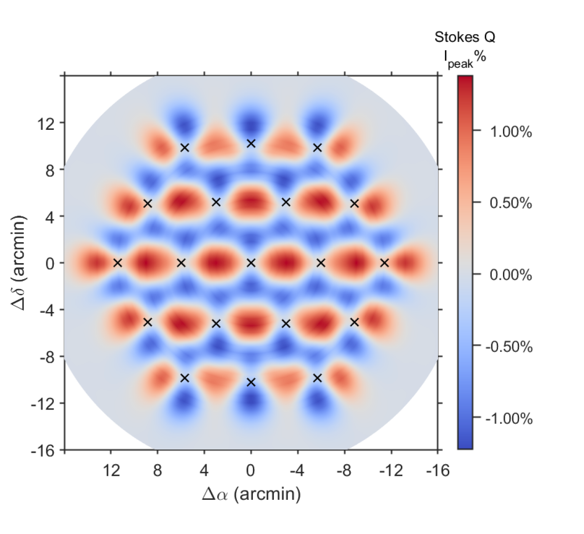
The Stokes , and mapping results of J1407+2827 for each individual beam together with the simulation results are depicted in Figures 12, 13, 14, 15, 16, and 17, respectively. As shown in these figures, Stokes is much noisier, with no clear beam structure detected in any of the beams. Stokes exhibits a clear beam squash structure: for the central and inner beams, this structure remains consistent, with positive lobes on either side (in red) clearly separated, while the center region shows negative values. Consequently, the negative lobes on both sides (in blue) form an almost continuous shape, creating a unified structure. In contrast, each outer beam displays a distinct squash pattern. Overall, the beam structure intensity across all beams is below 0.2 K, corresponding to 0.7% of the Stokes intensity, with no significant intensity difference between inner and outer beams. Notably, beam M12 demonstrates the highest squash intensity. The simulation predicts similar results, indicating that certain lobes in the outer beams’ squash structure are stretched, leading to a pattern distinct from that of the inner beams, while no intensity difference is observed between the inner and outer beams. In Stokes , the two-lobed squint structure and secondary structures are clearly evident in all beams. Comparing with the central beam, inner beams exhibit a more concentrated distribution in one direction that correlates strongly with the position angle. This effect is even more pronounced in the outer beams, where the structures are more compact, resulting in a significant increase in intensity due to the horns being displaced further from the focus. The beam squint orientation is distinctly observed in both the inner and outer beams, with the two-lobed squint structure aligning with the angle of each beam’s position angle. Overall, the Stokes intensity across all beams remains below 0.1 K, accounting for approximately 0.4% of the Stokes intensity, with the central beam demonstrating the best performance. These results align closely with the beam squint predictions by the simulation, particularly concerning the stretching of the lobes. For instance, the model of M08 clearly illustrates the positive and negative lobes being stretched into a horizontal configuration, which is in excellent agreement with the observed results. Additionally, the model also indicates that the intensity of the squint structure in the outer beams is significantly greater than that in the inner beams.
Figures 18, 19, and 20 depict the combined response of FAST in the Stokes , , and parameters for J1407+2827 together with the theoretical model. Intrinsic noise in Stokes , likely due to gain fluctuations in linearly polarized receivers, obscures the beam squash. Conversely, the performance of all beams in Stokes exhibits favorable characteristics, with responses from beam squashes having , ranging from K to 0.4 K. As mentioned above, beam M12 displays a more pronounced beam squash compared to other beams. For Stokes , it is observed that the combined response of all 19 beams displays beam squint intensity having , ranging from K to 0.3 K, indicating the highest level of performance among the Stokes , , and parameters. Due to data quality issues, the beam squash and squint structures exhibited in the combined response of the 19 beams differ somewhat from the results of the theoretical model; however, both show alternating positive and negative structures in Stokes and . Furthermore, numerous observed vertical and horizontal structures are present, indicating that these features are not artifacts of the data but rather the result of overlapping squash and squint structures from different beams. These findings affirm the exceptional capabilities of FAST in detecting the Stokes and parameters, providing a robust foundation for conducting in-depth investigations into the interstellar magnetic field, particularly concerning Zeeman multi-beam observations.
4 Conclusions
This study provides a comprehensive analysis to characterize the beam structures of the Five-hundred-meter Aperture Spherical radio Telescope (FAST) across the Stokes , , , and parameters, encompassing all 19 beams. We use an on-the-fly mapping pattern designed for simultaneous sky surveys using these 19 beams, directed towards polarization calibrators J1407+2827 and J0854+2006. The theoretical model was also developed, with the electromagnetic simulation packages CST and GRASP-10 used to compute the telescope’s complete radiation patterns across all Stokes parameters. Our investigation confirms the symmetry of the central beam and the asymmetry of the off-center beams. The central beam of FAST shows a symmetrical pattern without detectable sidelobes, which is significant as it indicates a well-behaved central beam, crucial for accurate observations. The off-center beams exhibit significant asymmetrical shapes; these shapes were modeled using log-normal and Gaussian methodologies. This asymmetry can affect the accuracy of data and needs to be accounted for in analyses.
Focusing on the Stokes parameter, we report fitting results revealing variations in , relative beam efficiency, , beam size, position angle, and . Our analysis concludes that inner beams demonstrate superior beam efficiency and beam size compared to outer beams. This suggests that the inner beams are more effective in collecting data and have better performance. The distribution of position angles demonstrates a consistent angular spacing of 29 degrees between the outer beams and 60 degrees between the inner beams, suggesting that the coma and sidelobes resulting from the lateral displacement of the feed horn primarily determine the position angle of each beam. Quantitative examination reveals that the sidelobe responses of the inner beams contribute approximately 2% of the main lobe flux, increasing to 5% for outer beams, with a peak at 6.8% of M16. This indicates that sidelobe contamination is relatively minor in the inner beams but more pronounced in outer beams. These results can provide valuable support for work related to data within the narrow frequency range centered at 1420.4 MHz.
Furthermore, we study the responses of FAST’s 19-beam receiver across the Stokes , , and parameters. The analysis of Stokes and reveals distinct beam squash and squint structures across the 19 beams. Stokes shows a clear four-lobed cloverleaf squash structure, particularly in the central and inner beams, where positive lobes are well-defined on either side, and negative values dominate the center region. Although the overall intensity across all beams remains below 0.2 K (0.7% of the Stokes intensity) without significant differences between inner and outer beams, beam M12 exhibits the highest squash intensity. The theoretical model supports these observations, indicating that certain lobes in the outer beams are stretched, resulting in a unique pattern distinct from the inner beams.
In Stokes , the two-lobed squint structure and a secondary eight-lobed structure featuring an alternating arrangement of positive and negative lobes are evident in all beams. Compared with the central beam, inner beams exhibit a more concentrated distribution in one direction that correlates strongly with the position angle. This trend is even more pronounced in the outer beams, where compact structures lead to increased intensity due to the horns’ displacement from the focus. The beam squint orientation aligns with the respective position angles, and the overall intensity in Stokes remains below 0.1 K (approximately 0.4% of the Stokes intensity), with the central beam performing the best. These findings align closely with the beam squint predictions by the simulation.
References
- Baars et al. (1977) Baars, J. W. M., Genzel, R., Pauliny-Toth, I. I. K., et al. 1977, A&A, 61, 99
- Baek et al. (2015) Baek, S.-J., Park, A., Ahn, Y.-J., et al. 2015, The Analyst, 140, 250. doi:10.1039/C4AN01061B
- Chang et al. (2015) Chang, C., Monstein, C., Refregier, A., et al. 2015, PASP, 127, 1131. doi:10.1086/683467
- Giovanelli et al. (2005) Giovanelli, R., Haynes, M. P., Kent, B. R., et al. 2005, AJ, 130, 2598. doi:10.1086/497431
- Guenther (1990) Guenther, R. D. 1990, Modern Optics, ISBN 0-471-60538-7. Wiley-VCH
- Heiles et al. (2001) Heiles, C., Perillat, P., Nolan, M., et al. 2001, PASP, 113, 1247. doi:10.1086/323290
- Heiles (2002) Heiles, C. 2002, Single-Dish Radio Astronomy: Techniques and Applications, 278, 131. doi:10.48550/arXiv.astro-ph/0107327
- Jiang et al. (2019) Jiang, P., Yue, Y., Gan, H., et al. 2019, Science China Physics, Mechanics, and Astronomy, 62, 959502. doi:10.1007/s11433-018-9376-1
- Jiang et al. (2020) Jiang, P., Tang, N.-Y., Hou, L.-G., et al. 2020, Research in Astronomy and Astrophysics, 20, 064. doi:10.1088/1674-4527/20/5/64
- Jing et al. (2024) Jing, Y., Wang, J., Xu, C., et al. 2024, Science China Physics, Mechanics, and Astronomy, 67, 259514. doi:10.1007/s11433-023-2333-8
- Kameno et al. (2021) Kameno, S., Cortes, P., Fomalont, E., et al. 2021, The Astronomer’s Telegram, 14952
- Kraus (1966) Kraus, J. D. 1966, New York: McGraw-Hill, 1966
- Li et al. (2018) Li, D., Wang, P., Qian, L., et al. 2018, IEEE Microwave Magazine, 19, 112. doi:10.1109/MMM.2018.2802178
- Liu et al. (2018) Liu, H. B., Hasegawa, Y., Ching, T.-C., et al. 2018, A&A, 617, A3. doi:10.1051/0004-6361/201832699
- Milligan (2005) Milligan, T. A. 2005, Modern Antenna Design, Wiley-IEEE Press, 2005
- Padmanabhan et al. (2015) Padmanabhan, H., Choudhury, T. R., & Refregier, A. 2015, MNRAS, 447, 3745. doi:10.1093/mnras/stu2702
- Pedrotti & Pedrotti (1993) Pedrotti, F. L. & Pedrotti, L. S. 1993, Introduction to Optics 2nd Edition, New Jersey: Prentice Hall
- Smith et al. (2017) Smith, S. L. et al. 2017, IEEE International Symposium on Antennas and Propagation & USNC/URSI National Radio Science Meeting, pp. 2137-2138, doi: 10.1109/APUSNCURSINRSM.2017.8073111.
- Staveley-Smith et al. (1996) Staveley-Smith, L., Wilson, W. E., Bird, T. S., et al. 1996, PASA, 13, 243. doi:10.1017/S1323358000020919
- Strong (1958) Strong, J. 1958, Concept of Classical Optics, San Francisco, CA: W.H. Freeman and Company
- Stutzman & Thiele (1981) Stutzman, W. L. & Thiele, G. A. 1981, New York, John Wiley and Sons
- Sun et al. (2021) Sun, X.-H., Meng, M.-N., Gao, X.-Y., et al. 2021, Research in Astronomy and Astrophysics, 21, 282. doi:10.1088/1674-4527/21/11/282
- Tello et al. (2013) Tello, C., Villela, T., Torres, S., et al. 2013, A&A, 556, A1. doi:10.1051/0004-6361/20079306
- Wang et al. (2022) Wang, Y., Zhang, Z., Zhang, H., et al. 2022, Astronomy and Computing, 39, 100568. doi:10.1016/j.ascom.2022.100568
- Du et al. (2022) Du, X., Islam, M., Robishaw, T., et al. 2022 International Conference on Electromagnetics in Advanced Applications (ICEAA), doi:10.1109/ICEAA49419.2022.9900055
- CST Studio Suite (2024) Dassault Systèmes Simulia Corp., https://www.3ds.com/products/simulia/cst-studio-suite
- GRASP (2024) TICRA, https://www.ticra.com/software/grasp/
- Potton (2004) Potton, R. J. 2004, Reports on Progress in Physics, 67, 717. doi:10.1088/0034-4885/67/5/R03
- Robishaw et al. (2021) Robishaw T., Heiles C. 2021, The WSPC Handbook of Astronomical Instrumentation, Chapter 6. doi: 10.1142/9789811203770_0006