Polarization Aware Movable Antenna
Abstract
This paper presents a polarization-aware movable antenna (PAMA) framework that integrates polarization effects into the design and optimization of movable antennas (MAs). While MAs have proven effective at boosting wireless communication performance, existing studies primarily focus on phase variations caused by different propagation paths and leverage antenna movements to maximize channel gains. This narrow focus limits the full potential of MAs. In this work, we introduce a polarization-aware channel model rooted in electromagnetic theory, unveiling a defining advantage of MAs over other wireless technologies such as precoding: the ability to optimize polarization matching. This new understanding enables PAMA to extend the applicability of MAs beyond radio-frequency, multipath-rich scenarios to higher-frequency bands, such as mmWave, even with a single line-of-sight (LOS) path. Our findings demonstrate that incorporating polarization considerations into MAs significantly enhances efficiency, link reliability, and data throughput, paving the way for more robust and efficient future wireless networks.
Index Terms:
Movable antenna, fluid antenna system, polarization, mmWave, MU-MISO.I Introduction
The relentless pursuit of high-speed and reliable wireless communication has become a cornerstone of modern technological advancement. Emerging applications such as autonomous vehicles, the artificial intelligence of things, and augmented reality demand seamless connectivity with unprecedented data rates and minimal latency[1, 2]. These evolving requirements are pushing the boundaries of existing wireless communication systems, necessitating innovative solutions to address challenges like spectrum scarcity, signal degradation, and dynamic environmental conditions.
One promising technique that has emerged to meet these challenges is the use of movable antennas (MAs) [3, 4, 5, 6], also known as fluid antenna systems (FAS) [7, 8, 9, 10, 11]. By dynamically adjusting the position and orientation of antennas, it is possible to achieve enhanced signal-to-noise ratio (SNR), wider coverage, and adaptability to changing environments and user locations, without solely relying on traditional methods like increasing transmission power, beamforming, or deploying additional infrastructure[12, 13, 14, 15, 16, 17].
Previous research has explored the applications of MAs and FAS in radio frequency bands characterized by rich multipath environments [3, 7]. In these settings, antenna movement is leveraged to exploit spatial diversity arising from amplitude fluctuations caused by multipath propagation.
In [7], the authors propose FAS that allows the receiving antenna to move to positions to capture the strongest signal. Analysis of outage probability demonstrates that, within a movement range of 0.2, FAS can achieve performance comparable to a maximal ratio combining system with five antennas spanning 2. This flexibility in antenna positioning offers significant advantages, especially in scenarios requiring massive connectivity. It allows each user to find an optimal position where instantaneous interference is minimized, effectively creating deep nulls. This spatial multiplexing gain facilitates multi-user access, a concept introduced as Fluid Antenna Multiple Access (FAMA) in [8]. Building upon this concept, [9] extends FAS to a two-dimensional (2D) implementation and discusses reconfigurable pixel technologies as a practical approach for realization. Additionally, [18] introduces a continuous FAS (CFAS) architecture, demonstrating that CFAS outperforms discrete FAS with limited ports, particularly at medium to high threshold levels.
The MA system presented in [3] exhibits additional phase variations due to antenna translation, significantly surpassing fixed-position antennas in both deterministic and stochastic channels. The system’s performance further improves with increased positioning accuracy, larger movement ranges, and enhanced multipath effects. Building on 2D MA system, advancements in six-dimensional (6D) systems, such as those discussed in [4], enable simultaneous three-dimensional (3D) translation and rotation, enhancing the system’s directional capabilities. By imposing spatial constraints on surfaces equipped with 6D movable antennas (6DMA), user interference is reduced, improving the signal-to-interference-plus-noise ratio (SINR). In [5], the 6DMA model is simplified by integrating conventional fixed-position antenna arrays with 6DMA surfaces capable of rotating along a circular path. By limiting the degrees of freedom for surface movement to the azimuth angle along the circular track, computational complexity is significantly reduced while enhancing the system’s maximum capacity.
Despite these advancements, the impact of polarization changes due to antenna movement and rotation has been largely overlooked. Polarization is a fundamental characteristic of electromagnetic waves, describing the orientation of the electric field vector as the wave propagates through space [19, 20, 21, 22, 23]. In wireless communication systems, proper alignment of polarization between transmitting and receiving antennas is crucial for efficient signal transmission and reception. When polarizations are properly aligned, the receiving antenna can maximally capture the transmitted energy, resulting in stronger signal strength, improved SNR, and enhanced overall system performance. Conversely, polarization mismatch occurs when there is a misalignment between the polarization orientations of the transmitting and receiving antennas, leading to significant signal attenuation as the misaligned component of the electromagnetic wave is effectively lost. Neglecting polarization effects can lead to incomplete system models and suboptimal performance assessments, hindering a full understanding of the impact and advantages of MAs.
This oversight is particularly critical as communication systems move towards higher frequency bands, such as the millimeter-wave (mmWave) spectrum [24, 25]. At these higher frequencies, signal propagation becomes more directional with reduced diffraction around obstacles, often resulting in a single line-of-sight (LOS) link between transmitter and receiver [26]. Previously, it was believed that MAs offer no gains in such LOS scenarios due to the lack of multipath diversity [7, 3]. However, our formulation incorporating polarization effects indicates otherwise – MAs can achieve significant performance gains even in LOS scenarios by facilitating polarization matching. As such, there is a clear gap in current research: the need to incorporate polarization effects into the design and optimization of MA systems, especially as the wireless industry advances towards higher frequency bands to achieve greater bandwidths and data rates.
To fill the gap, this paper makes the following main contributions:
-
•
We introduce a polarization-aware movable antenna (PAMA) framework, which incorporates polarization effects into the design and optimization of antenna movement and rotation. PAMA uncovers a previously overlooked, but defining benefit of antenna movement – facilitating optimal polarization matching between the transmitter and receiver. By accounting for the impact of polarization changes due to movement and rotation, PAMA provides a more refined system model and deepens our understanding of the dynamic capabilities of MAs.
-
•
Building upon the electromagnetic theory, we develop a polarization-aware channel model that describes the impact of 3D movement and rotation of antennas on the channel gains. Grounded in Maxwell’s equations, this model allows for precise characterization of how antenna positioning and orientation affect polarization alignment and, consequently, signal reception quality. By integrating these factors into the system design, we enable the optimization of antenna movements to maintain polarization alignment, thereby maximizing the sum rate of the communication system.
-
•
Contrary to prior beliefs that MAs are more effective in low-frequency, multipath-rich environments, our PAMA framework demonstrates that MAs are highly effective in higher frequency bands such as the mmWave band, even with a single LOS link. The smaller size of antennas at higher frequencies makes them easier to move and rotate, facilitating practical implementation of PAMA systems in these bands. This new understanding extends the potential and application of MA to next-generation wireless communication systems that demand higher bandwidths.
Organization: The remainder of this paper is structured as follows. Section II introduces the system model and essential geometric concepts used throughout the work. Section III presents our PAMA framework and the polarization-aware channel model. Section IV explores the impacts of 3D antenna translation and rotation on the PAMA channel gains. Section V demonstrates the potential of PAMA through a sum-rate optimization problem. Finally, Section VI concludes the paper.
Notations: We use boldface lowercase letters to denote column vectors (e.g., , ) and boldface uppercase letters to denote matrices (e.g., , ). For a vector or matrix, denotes the transpose, denotes the complex conjugate, and denotes the conjugate transpose. stand for the sets of complex values. The imaginary unit is represented by . The Euclidean norm of a vector is denoted by . For two vectors and , denotes the angle between them, and denotes their inner product.
II System Model
We consider a mobile edge network within a 3D environment. The network comprises a base station (BS) and mobile users distributed within the 3D space. The BS is equipped with half-wave dipole antennas, and each mobile user is equipped with a single half-wave dipole antenna. We focus on the downlink transmission from the BS to the users, operating in the mmWave frequency band. Both the antennas at the BS and mobile users are movable.
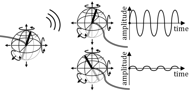
Definition 1 (Movable Antennas).
A movable antenna is capable of performing 3D translations and 3D rotations, allowing it to navigate through and orient within 3D space, as depicted in Fig. 1.
Translation typically requires larger operational spaces, often spanning tens of wavelengths, whereas rotation can be accommodated within a more compact area, approximately the size of a half-wavelength sphere, as shown in Fig. 1. In this work, we assume that the antennas on mobile users are restricted to 3D rotation, due to the spatial constraint. In contrast, the antennas at the BS can perform both 3D rotation and translation independently within a designated region. The extension of this model to include translatable antennas for mobile users is straightforward.
In this work, we consider the far-field scenario, which implies the following:
-
•
Plane wave. The waves received by the users can be treated as plane waves because the propagation distance is much greater than the wavelength and the dimensions of the movable regions.
-
•
Point representation of antennas. The physical sizes of the transmitting and receiving antennas are negligible compared to the propagation distance, allowing us to represent their positions as points specified by their center coordinates.
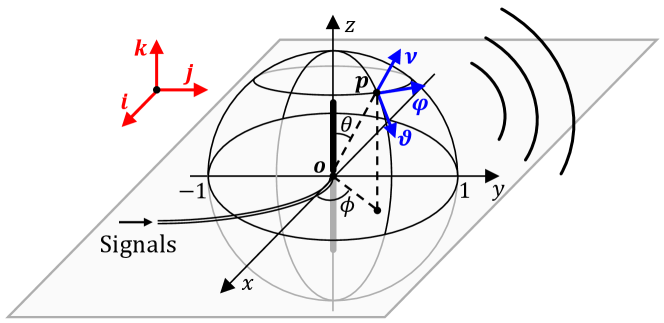
To mathematically represent the network and the positions of the antennas, we establish two coordinate systems: the Cartesian Coordinate System (CCS) and the Spherical Coordinate System (SCS), as depicted in Fig. 2.
Definition 2 (Coordinate Systems).
We define a CCS to describe the positions of the transmitting and receiving antennas, with three orthogonal unit vectors denoted as , , and .
Correspondingly, an SCS is established with its origin at point in the CCS, and the direction of serving as the reference axis. The SCS has three unit vectors: the radial unit vector , the polar angle unit vector , and the azimuthal angle unit vector .
| Dot products | |||
Table I provides the conversion formulas between the unit vectors of the two coordinate systems. For instance, the radial unit vector in the SCS can be expressed in terms of the CCS unit vectors as .
Given the two coordinate systems, we introduce several definitions regarding the antennas’ positions and orientations.
Definition 3 (Positions of the Antennas).
In the far-field scenario, the position of an antenna can be represented by its center coordinates. We denote the center coordinate of the -th transmitting antennas at the BS by , . Similarly, the center coordinate of the receiving antenna at the -th user is denoted by for .
Definition 4 (Directions of Antennas).
The direction of an antenna, characterized by a unit vector , is the orientation in which the antenna is pointed. We denote the direction for the -th transmitting antenna at the BS by , and for the receiving antenna at the -th user by .
Definition 5 (Polar and Azimuthal Angles of Antennas).
The polar angle of an antenna, denoted by , is the angle between and the direction of the antenna. The azimuthal angle of an antenna, denoted by , is the angle measured counterclockwise from to the projection of the antenna onto the plane. For the -th transmitting antenna, these angles are denoted by and , respectively. For the receiving antenna at the -th user, they are denoted by and , respectively.
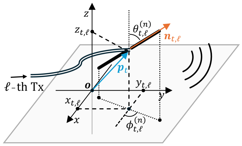
The polar and azimuthal angles are illustrated in Fig. 3. A summary of the definitions and their geometric relationships is given in Tab. II.
Lemma 1.
The direction of an antenna in the CCS can be represented by its polar and azimuthal angles. For the -th transmitting antenna, we have
| (1) |
The CCS representation facilitates mathematical operations such as dot products, providing computational simplicity. In contrast, the SCS representation offers a clearer depiction of the relationship between channel gains and antenna orientation.
III The PAMA Framework
Building upon the system model, this section presents our PAMA framework. At the core of wireless communication is the interaction between transmitting and receiving antennas through electromagnetic fields. An alternating current in the transmitting antenna generates electromagnetic waves, creating an electromagnetic field that propagates through space to the receiver. The receiving antenna interacts with this field, specifically sensing the electric field component, which induces a current within the antenna used to recover the transmitted signal. This fundamental interaction is governed by Maxwell’s equations, which describe how electric and magnetic fields are generated by charges and currents, and how they propagate in space.
In this section, we begin by modeling the radiation of the electric field from movable transmitting antennas, characterizing how movements – 3D translations and rotations – affect the spatial distribution and polarization of the emitted electromagnetic waves. We then explore how movable receiving antennas detect and interact with the electric field. Ultimately, the analysis leads to a polarization-aware channel representation for movable antennas.
III-A Electric field radiation
Given that the electric field at the receiver is a superposition of waves from all transmitting antennas, we can focus on the radiation analysis of a single antenna. To facilitate the exposition, we introduce the emission angle of a transmitting antenna.
Definition 6 (Emission Angle).
The emission angle is the angle between the direction of the transmitting antenna and the propagation direction of the electromagnetic wave from the antenna to an observation point . The emission angle of the -th transmitting antenna can be written as
| (2) |
where .
Theorem 2 below summarizes the main result of this section.
Theorem 2 (Electric Field Radiation).
Consider the -th transmitting antenna located at and oriented in the direction . Suppose the transmitted signal at -th antenna is . At any observation point in space, the electric field induced by this antenna is given by
| (3) | |||
where denotes the complex amplitude of the induced electric field, incorporating both magnitude and phase; denotes the polarization direction of the electromagnetic wave at point ; is the speed of light; is the magnetic permeability of air, is the wavelength.
| For -th transmitting antenna | For -th receiving antenna | ||
| Position | Position | ||
| Direction | Polar Angle: , Azimuthal Angle: | Direction | Polar Angle: , Azimuthal Angle: |
| Emission Angle | , with | Incident Angle | , with |
| Transmitted Angle | , with | ||
Proof.
We start by considering a reference scenario where the dipole antenna is stationary, located at the origin , and oriented along the direction . When transmitting signal , the current density applied to the dipole can be written as [19]
| (4) |
where is the maximum current. Without loss of generality, we set .
In the mmWave band, signal diffraction and scattering are minimal, making non-line-of-sight (NLOS) paths significantly weaker than the LOS path.111As a concrete example, LOS signals can be over dB stronger than the NLOS signal at a distance of 100 meters, according to the mmWave channel specified in 3GPP TR 38.901 [26]. Therefore, we only consider the LOS component.
The electric field radiated by the stationary transmitting antenna at any point in space is given by
| (5) |
where is the emission angle between and , and . The unit vector is the polarization direction at . Eq. (5) is a classical result in electromagnetic theory [19, 27] and provides the foundation for our analysis. In Appendix A we provide a detailed derivation of this equation from Maxwell’s equations.
We next consider the antenna movement. After translation and rotation, the -th antenna moves to with a direction . The complex amplitude of the induced electric field follows from (5) and can be written as
| (6) |
where is the emission angle from to . Under the far-field condition, and can be treated parallel, hence we have
Therefore, (6) can be refined as
| (7) |
where the approximation follows from . Note that the term in the exponent indicates that the phase varies with distance on the order of the wavelength, hence the term in the exponent cannot be neglected.
At point , the polarization direction of the electric field is perpendicular to the propagation direction, and lies in the plane formed by the direction of the transmitting antenna and the propagation direction. Thus, the polarization direction can be obtained by subtracting the component along the propagation direction from the direction of the transmitting antenna, yielding
| (8) |
Eq. (3) reveals that, at a given observation point , both the complex amplitude and the polarization of the electric field are affected by the movement of the transmitting antenna.
Corollary 3.
The magnitude of the electric field
| (9) |
first increases and then decreases as a function of , reaching its maximum value when . This variation depends solely on the emission angle, which results from the 3D orientation of the transmitting antenna.
Proof.
See Appendix B. ∎
This paper focuses on the half-wave dipole, the most fundamental type of antenna, to develop the PAMA framework. The dipole antenna is directional in the 3D space: when positioned vertically, it radiates uniformly in the horizontal plane but has directional properties in the vertical plane. Our PAMA framework is sufficiently versatile to extend to more complex directional antennas, provided their radiation patterns are known.
III-B Electric Field Sensing
Theorem 2 establishes the electric field induced by a movable transmitting antenna. In this section, we explore how a movable receiving antenna senses the electric field.
The process of capturing radio waves with a receiving antenna involves the transmission of electromagnetic waves from air into the antenna. Dipoles emit linearly polarized radio waves, and when such a plane wave reaches the boundary between the air and the antenna, part of the wave is reflected back into the air, while the remainder is transmitted into the antenna.
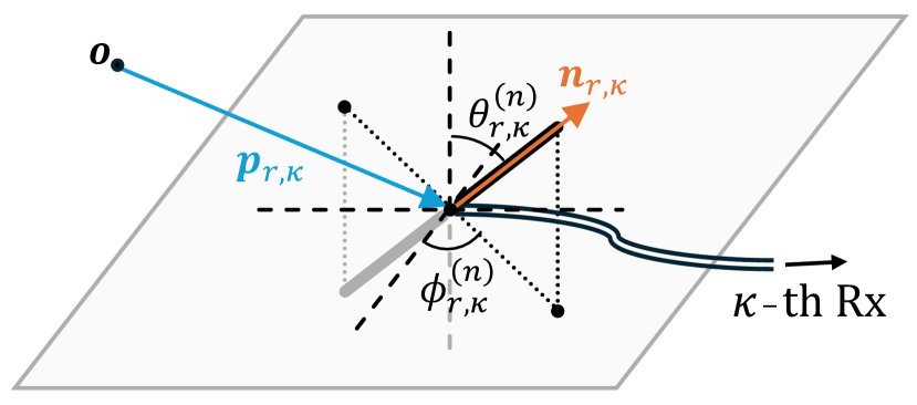
Definition 7 (Incident Angle).
The incident angle is the angle between the direction of the incoming electromagnetic wave and the normal to the surface of the antenna at the point of impact. The direction of the normal can be obtained by subtracting the component that is collinear with the receiving antenna from the direction of the incident electromagnetic wave :
| (10) |
We denote by the incident angle of the wave from the -th transmitting antenna to the -th receiving antenna.
Definition 8 (Transmitted Angle).
The transmitted angle is the angle between the normal of the receiving antenna and the new propagation direction of the electromagnetic wave inside the antenna after it has entered.
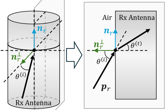
An illustration of the incident angle and transmitted angle is shown in Fig. 4
Definition 9 (Permittivity and Permeability).
Permittivity quantifies the ability of a material to store electrical energy in an electric field. Permeability is a measure of how easy or difficult it is for a magnetic field to pass through a material [27]. We define and as the permittivity of air and antenna, respectively, and and as the permeability of air and antenna, respectively. We further define a relative permittivity
| (11) |
Lemma 4 (Snell’s law [28]).
Let and be the permittivity of air and antenna, respectively, and and be the permeability of air and antenna, respectively. We have
| (12) |
A critical aspect of electric field sensing is polarization matching, which refers to the alignment of the transmitting and receiving antennas’ polarization states. The efficiency of polarization matching determines how much energy is transferred into the antenna. Therefore, effective polarization matching is essential for maximizing the power transfer and minimizing signal degradation, especially in systems with movable antennas where orientation can dynamically change.
Definition 10 (Polarization Matching Angle).
The polarization matching angle is the angle between the polarization direction of the incident wave and the direction of the receiving antenna. We denote by the polarization matching angle of the wave emitted from the -th transmitting antenna to the -th receiving antenna.
Theorem 5 below summarizes the main result of this section.
Theorem 5 (Electric Field Sensing).
Consider the signal transmitted from the -th transmitting antenna. The received signal at the -th user’ antenna can be written as
| (13) | |||
where is the complex amplitude of the induced electric field by the -th antenna at ; the constant is an antenna factor for converting field amplitude to voltage; denotes the polarization matching efficiency, considering both the polarization matching angle and energy reflection; and are the energy reflection coefficients for the horizontal and vertical polarization:
| (14) | |||
| (15) |
Proof.
The electric field induced by the -th transmitting antenna possesses a polarization direction . The -th receiving antenna, oriented at , has a polarization matching angle w.r.t. the incident wave. We can partition the incident polarization into horizontal and vertical components.
Due to the electromagnetic boundary conditions at the interface of different media (air to antenna), part of the energy of each polarization component is reflected. The reflection coefficients and , corresponding to horizontal and vertical polarizations respectively, determine how much of the incident wave’s energy is transmitted into the receiver.
The reflection coefficient for any polarization can generally be expressed in terms of the characteristic impedances of the interacting media [27, 21]:
| (16) |
where
Given (16), we compute the reflection coefficients for the horizontal and vertical components:
| (17) | |||
| (18) |
where (a) follows because the permeability of most materials remains constant and is unaffected by changes in frequency or temperature [21]. Therefore, we have .
Without loss of generality, this paper represents the received signal by the voltage induced at the receiver. In practice, the difference between the amplitude of the received signal in terms of voltage and current is simply a scaling factor: the resistance, which can be considered part of the antenna factor. Therefore, the received signal, i.e., the induced voltage, at the -th user from the -th transmitting antenna can be written as
where the constant is the antenna factor for converting field amplitude to voltage, as shown in (13). ∎
III-C Polarization-aware channel gain
Building upon Theorems 2 and 5, this section characterizes the polarization-aware channel gain for movable transmitting and receiving antennas.
Theorem 6 (PAMA Channel Gain).
Consider the transmission from the -th transmitting antenna to the -th receiving antenna. The polarization-aware channel gain is given by
| (19) | |||
where .
The PAMA channel gain model captures the changes induced by the radiation pattern, the polarization matching efficiency, and phase shifts as the antenna translates and rotates. Compared to existing channel models for MAs that primarily focus on the phase changes, our PAMA model offers a more comprehensive and rigorous framework to explore the potential of MAs, enabling deeper analysis and performance assessment.
IV Impacts of Antenna Movements
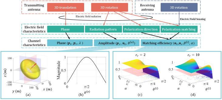
This section analyzes the PAMA channel model and examines how each variable influences channel quality, providing insights into the key characteristics of PAMA and identifying the sources of its performance gains. Fig. 5 summarizes the relationships between antenna movement and their corresponding impacts on the channel. It is essential to highlight that these properties are derived under the conditions of a far-field scenario and a dominant LOS path. For clarity, the indices and in the subscripts are omitted in this section.
Proposition 1.
Antenna translation only contributes a phase term to the PAMA channel gain. This implies that the effect of antenna translation can be fully realized by precoding.
In the far-field LOS scenario, the electromagnetic waves can be approximated as plane waves, and the spatial fading characteristics are negligible. The relative orientation of the electric field vectors between the transmitter and receiver remains unchanged despite antenna translation. This means that antenna translation does not affect the amplitude or polarization alignment of the received signal – only the phase changes due to the difference in path length, leading to Proposition 1.
In practical systems, digital precoding is often easier to implement than mechanical antenna movements. Therefore, when studying MAs, it is essential to consider the unique advantages that MAs introduce beyond what precoding can achieve. Proposition 1 indicates that the benefits of antenna translation are more significant in near-field or rich multi-path environments, in which case antenna translation can impact the amplitude and spatial characteristics of the channel gain, offering advantages that precoding alone cannot replicate.
In the context of this paper, which focuses on far-field and mmWave dominant LOS paths, the unique gains that MAs can offer over precoding are primarily obtained through antenna rotation rather than translation.
Proposition 2.
The rotation of the transmitting antenna alters the amplitude of the channel gain by modifying both the radiation pattern of the induced electric field and the polarization matching efficiency at the receiver.
When the transmitting antenna rotates, it changes the emission angle of the electromagnetic wave. This alteration affects the antenna’s radiation pattern – the distribution of the electric field w.r.t. the CCS – which in turn influences the electric field intensity received. As illustrated in Fig. 5 (a) and (b), different emission angles lead to variations in the radiation pattern, resulting in changes to the received signal’s strength. According to Corollary 3, the magnitude or intensity of the electric field reaches its maximum when the emission angle is . To achieve this, the transmitting antenna should be positioned within the plane that is perpendicular to the direction of wave propagation.
Furthermore, the rotation of the transmitting antenna also modifies its polarization orientation, thereby changing the polarization matching angle between the transmitter and receiver, and hence the matching efficiency in the PAMA channel gain.
Proposition 3.
The rotation of the receiving antennas alters the amplitude of the channel gain by modifying the polarization matching efficiency.
Rotating the receiving antennas affects both the incident angle of the incoming electromagnetic wave and the polarization matching angle , both of which impacts the polarization matching efficiency.
-
1.
The change of the incident angle alters the energy reflection coefficients and , as defined in (14) and (15). These reflection coefficients characterize the proportion of electromagnetic energy that enters the antenna. A smaller reflection coefficient indicates that more energy is transmitted into the antenna, enhancing the received signal strength.
-
2.
The orientation of the receiving antenna relative to the electric field vector of the incoming wave determines the polarization matching angle , which describes the ratio of the horizontal to vertical components of the electromagnetic wave’s polarization relative to the antenna’s orientation. A better alignment (i.e., a smaller mismatch angle) leads to higher polarization matching efficiency.
Figs. 5 (c) and (d) illustrate how the polarization matching efficiency varies with the incident angle and the polarization matching angle for antennas with different relative dielectric constants . As can be seen, without proper optimization of the receiving antenna’s rotation, the matching efficiency can decrease significantly, potentially dropping to zero. In such cases, the antenna fails to effectively receive the incoming signal, resulting in a loss of information. Therefore, careful control of the receiving antenna’s orientation is essential for maximizing the channel gain and ensuring reliable communication in the PAMA framework.
Propositions 2 and 3 indicate that the amplitude of the channel gain is influenced by the orientations of both the transmitting and receiving antennas. To illustrate the extent to which antenna rotations affect the channel amplitude, we simulate two scenarios:
-
•
Scenario 1: Rotatable transmitting antenna with fixed receiving antenna;
-
•
Scenario 2: Fixed transmitting antenna with rotatable receiving antenna.
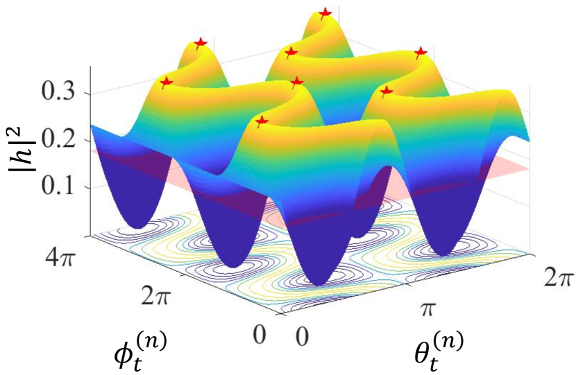
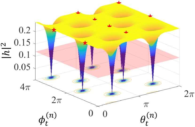
In the simulations, the positions of the antennas are set as , . The fixed antennas are oriented vertically upward, with a direction vector of . For visualization purposes, we vary the polar and azimuthal angles of the rotatable antennas over two periods, even though their actual values lie within a single period. The channel amplitude variations for the two scenarios are presented in Figs. 6(a) and 7(a), respectively.
For scenario 1 with a fixed receiving antenna, Fig. 6(a) shows that a randomly oriented transmitting antenna has only a probability of delivering at least half of the maximum possible energy to the user. Each period can yield two sets of maximum values due to the symmetry of the dipole antennas, where the collinear reverse sets of polar and azimuthal angles provide equivalent performance.
For scenario 2 with a fixed transmitting antenna, Fig. 7(a) shows that a randomly oriented receiving antenna has a probability of capturing at least half of the maximum energy. However, the remaining of orientations present a significant risk of receiving virtually no energy. This outcome highlights the critical importance of antenna orientation in ensuring reliable communication.
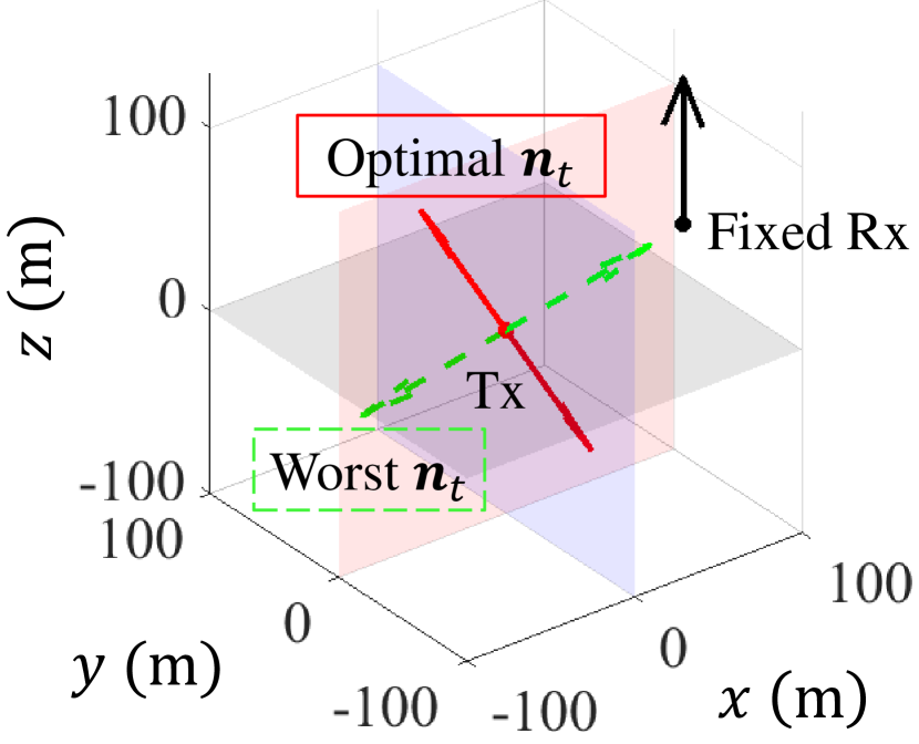
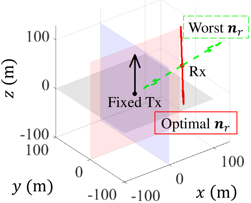
Figs. 6(b) and 7(b) depict the positions and orientations of the transmitting and receiving antennas for both scenarios. In these illustrations, fixed Antennas are shown with vertical black arrows; the optimal orientations of the rotatable antennas are shown with solid red arrows, indicating the directions that maximize the channel gain; the worst-case orientations of the rotatable antennas are shown with dashed green arrows, representing the directions that minimize the channel gain.
Proposition 4.
In a single-input single-output (SISO) PAMA system:
-
1.
Optimal orientation: The best channel gain is achieved when the transmitting and receiving antennas are oriented such that they, along with the propagation path, lie within the same plane.
-
2.
Worst orientation: The poorest channel gain occurs when one antenna points directly at the other.
When the electromagnetic field reaches the receiving antenna, it can be decomposed into three orthogonal components along: the direction of the receiving antenna ; the normal direction of the incident signal ; a direction perpendicular to both and , denoted by . This decomposition is illustrated in Fig. 8. The component along represents the horizontal polarization component, while the components along and represent the vertical polarization components.
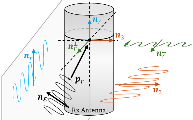
According to (14) and (15), we have , meaning that the horizontal polarization component has a smaller reflection coefficient, and thus a better matching efficiency, than the vertical component. Therefore, increasing the component along by adjusting antenna orientations enhances the channel gain. However, achieving complete horizontal polarization requires the polarization matching angle to be zero, which also corresponds to an incident angle of zero. Under this condition, the reflection coefficient increases, reducing the matching efficiency. Therefore, simply minimizing is suboptimal. Instead, we need to balance the horizontal and vertical polarization components to maximize the overall matching efficiency.
Since the polarization direction is perpendicular to the propagation direction, and is perpendicular to the antenna direction, the polarization matching angle satisfies . To increase the incident angle and reduce the reflection coefficient without introducing additional vertical polarization components along , it is optimal to maintain . For linearly polarized antennas, this configuration implies that the transmitting antenna, the receiving antenna, and the propagation path are all aligned within the same plane, confirming Proposition 4. It is important to note that lying in the same plane does not necessarily mean that the transmitting and receiving antennas are parallel, as depicted in Figs. 6(a) and 7(a).
Figs. 6(b) and 7(b) demonstrate that the worst-case orientation consistently occurs when one antenna is directed toward the other. This phenomenon is explained by:
-
•
For the transmitting antenna in Figs. 6(b), when the emission angle , meaning the transmitting antenna points directly at the receiver, the electric field intensity in that direction is effectively zero due to the dipole antenna’s radiation pattern.
-
•
For the receiving antenna in Figs. 7(b), when the incident angle , the reflection coefficients , indicating total reflection with no energy entering the antenna. Additionally, the polarization matching angle , indicating complete polarization mismatch and resulting in zero capturable energy.
V Optimization with PAMA
By incorporating polarization, we have redefined movable antennas and established more refined, polarization-aware channel models. This enhancement serves as a foundation for further optimizations, specifically tailored to harness the dynamic adjustments of antenna orientations and positions to maximize system performance. In this paper, we focus on the fundamental sum-rate optimization [13] to reveal the potential of PAMA.
V-A Sum-rate optimization
We consider a multi-user multiple input single output (MU-MISO) configuration where the BS serves users simultaneously, , using transmit beamforming. Let the source data symbols intended for the users be , where the symbol power is normalized such that , . The beamforming vector for the -th user is denoted by , with individual elements . A power scaling matrix, defined as , is employed to control the power distribution among the users. After beamforming, the signal transmitted from the BS antennas, denoted by , is written as
| (20) |
subject to the constraint , where denotes the total power constraint.
The symbols received by the users, denoted by , are given by
| (21) |
where is the channel matrix with the elements defined by (19); is the precoding matrix; is the additive white Gaussian noise (AWGN) vector, where .
At each user , the SINR is defined as
| (22) |
and the achievable rate is
| (23) |
The average achievable rate across all users is
| (24) |
with the equivalent total SINR for the system:
| (25) |
Our goal is to maximize the equivalent total SINR of the system by jointly optimizing the positions and orientations of the transmitting antennas, the orientations of the receiving antennas, beamforming matrix , and the power scaling matrix . The optimization problem is formulated as
| (P1): | (26a) | |||
| s.t. | (26b) | |||
| (26c) | ||||
| (26d) | ||||
In constraint (26c), a minimum separation of between any two antennas is imposed to prevent collisions. The term in (26d) represents the movable region of the transmitting antennas.
To solve (P1), we employ zero-forcing (ZF) beamforming, which can fully eliminate the inter-channel interferences [29]. The ZF beamformer is given by
| (27) |
Since ZF beamforming completely removes interferences, the power allocation matrix can be easily obtained by water-filling [30], yielding
| (28) |
where is the water level that can be determined iteratively to satisfy the total power constraint.
Next, we transform the non-convex feasible region of into a convex set by linearizing the non-convex constraint in (26c) [4]. During the -th iteration of the gradient descent, considering the position from the previous iteration and the position (, ), we linearize by determining the intersection of the displacement vector with the spherical boundary . The boundary point is given by
A hyperplane is then defined w.r.t. and the vector as
and the corresponding closed halfspace divided by this hyperplane is given by
which includes and any vector that forms an acute angle with the vector .
By setting in (V-A), the non-convex constraint (26c) can be approximated as the following linear inequality:
| (29) |
Thus, problem (P1) is redefined to a more tractable form
| (P2): | (30a) | |||
| s.t. | (30b) | |||
Problem (P2) can be solved efficiently using alternating optimization and projected gradient descent.
Remark 1 (Translation versus beamforming).
With ZF beamforming, the phase shifts introduced by antenna translation are entirely compensated. The equivalent channel matrix reduces to a diagonal form, with each diagonal element given by .
In this MU-MISO scenario, the effect of antenna translation can be fully replicated through precoding. Therefore, the optimization problem (P1) can be solved without considering the optimization of the antenna positions . The constraints (26c) and (26d) can also be omitted. This conclusion is supported by our simulations depicted in Fig. 10, which show that antenna translation brings no benefits during the optimization of (P2).
Remark 2 (Channel estimation in PAMA).
Channel estimation poses a significant challenge in MA systems because determining the optimal antenna position requires knowledge of the channel characteristics at every possible position and orientation within the movement region . This task is particularly complex in radio frequency bands with rich multipath environments.
However, within our PAMA framework operating in the mmWave band, channel estimation is considerably simplified due to the dominance of the LOS path. PAMA only requires information about user positions and antenna orientations. With this information, we can accurately infer the channel gains at any position and orientation using (19).
Remark 3 (The case).
ZF beamforming effectively eliminates inter-user interference only when the number of users does not exceed the number of transmit antennas . When , we can partition the users into groups of size up to and assign orthogonal resources to each group. Alternatively, exploring different optimization criteria, such as minimizing interference leakage [31], can lead to alternative beamforming designs.
V-B Numerical simulations
| Symbol | Description | Value |
| Carrier frequency | 30 GHz | |
| Wave length | 0.01 m | |
| Noise power | -20 dBm | |
| Signal power | 0.5 W | |
| Relative permittivity | 2 | |
| Permeability | ||
| Antenna factor | 1 | |
| Transmitter region | ||
| #transmitting antennas | 8 | |
| #users |
This section presents numerical simulations to evaluate the performance of our PAMA framework in the context of sum-rate optimization. In the simulations, we consider users uniformly distributed within a 3D coverage area – a cube with dimensions of meters by meters by meters – centered at the origin of the CCS. Unless specified otherwise, the simulation parameters used are summarized in Tab. III. The BS is equipped with antennas, and the number of users varies among .
V-B1 Impact of polarization matching
Our PAMA framework integrates polarization effects into MAs and reveals a significant advantage of MAs: the ability to achieve optimal polarization alignment between the transmitter and receiver. To validate this capability, we consider the following antenna configurations within the PAMA framework:
-
•
Configuration 1: Transmitting antennas are randomly positioned and oriented; receiving antennas have random orientations.
-
•
Configuration 2: Transmitting antennas have optimized positions but random orientations; receiving antennas have random orientations.
-
•
Configuration 3: Both the positions and orientations of the transmitting antennas are optimized; receiving antennas have random orientations.
-
•
Configuration 4: Transmitting antennas are randomly positioned and oriented; the orientations of the receiving antennas are optimized.
-
•
Configuration 5: Both the positions and orientations of the transmitting antennas are optimized; the orientations of the receiving antennas are also optimized.
In Configurations 1 and 2, there is no optimization of polarization matching in the system. In Configuration 3, polarization matching is optimized by adjusting the orientations of the transmitting antennas. In Configuration 4, polarization matching is optimized by adjusting the orientations of the receiving antennas. In Configuration 5, polarization matching is optimized by adjusting the orientations of both transmitting and receiving antennas.
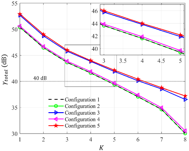
The simulation results for the configurations described above are illustrated in Fig. 10, where we evaluate the equivalent total SNR against the number of users, with the number of transmitting antennas set to . The following observations can be made:
-
•
As the number of users increases, the equivalent total system SNR decreases. With more users sharing the same transmission resources, each user receives less focused beamforming gain.
-
•
The performance curves of configurations 1 and 2 overlap, indicating that antenna translation does not provide any additional benefits. This occurs because the effect of antenna translation can be fully replicated through precoding, as explained in Remark 1.
-
•
When comparing configuration 3 to configuration 1, we find that optimizing polarization matching by rotating the transmitting antennas effectively enhances the equivalent SNR. The SNR gain increases with the number of users and averages around dB. If we aim for a target SNR of dB, the system can support one additional user by employing polarization matching through transmitting antenna rotation.
-
•
Comparing configuration 4 with configuration 1 reveals that optimizing polarization matching by rotating the receiving antennas provides minimal gain. This observation aligns with the analysis in Fig. 7, which shows that randomly oriented receiving antennas have approximately a probability of capturing at least half of the maximum signal energy. However, optimizing the orientation of the receiving antennas remains important for reducing outage probability, as there is still a small chance – less than – of complete signal loss without such optimization.
-
•
As expected, configuration 5 achieves the highest system gain and effectively mitigates the decline in equivalent SNR as the number of users increases. This outcome confirms the effectiveness of the PAMA framework in optimizing polarization matching between the transmitter and receiver, thereby enhancing overall system performance.
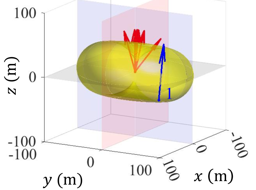
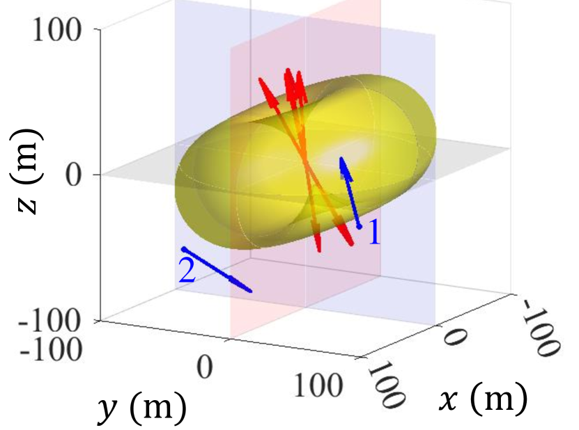
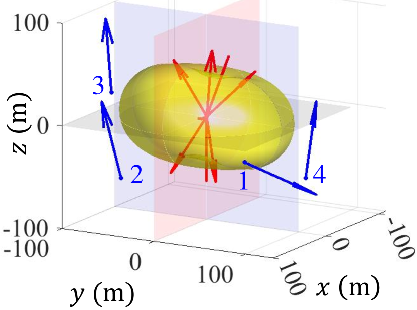
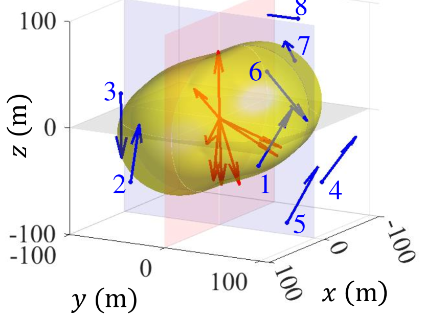
To provide a clearer understanding of the optimized PAMA in configuration 5, we present in Fig. 9 the optimal orientations of both the transmitting and receiving antennas as the number of users increases, along with the corresponding electric field isosurfaces.
-
•
In the single-user scenario illustrated in Fig. 9(a), all transmitting antennas are oriented to focus their maximum radiation patterns toward the target. The combined electric field distribution from the eight antennas resembles that of a single half-wavelength dipole antenna, forming a characteristic doughnut-shaped pattern.
-
•
As the number of users increases, the electric field distribution becomes more isotropic to effectively accommodate all users’ requirements.
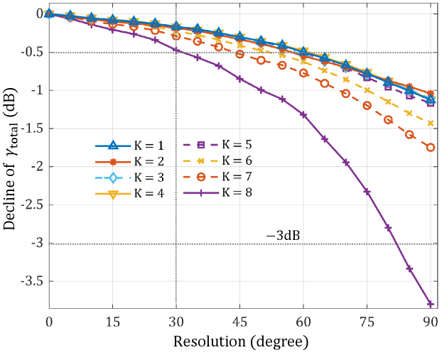
V-B2 Impact of antenna rotation granularity
Implementing PAMA in practice faces the challenge of precisely controlling the rotations of both transmitting and receiving antennas. While the simulation results in Fig. 10 assume infinite control precision, real-world systems are constrained by finite rotation granularity. To assess how rotation granularity affects system performance, we quantize the polar and azimuthal angles of the transmitting and receiving antennas, i.e., , , , and . We then evaluate the decline in the equivalent total SNR, , across different quantization levels. The simulation results are depicted in Fig. 11, where a resolution level of corresponds to the optimal orientation with infinite precision.
The findings show that the negative impact of reduced quantization precision on becomes more pronounced as the number of users increases. For example, with a rotation precision limited to , a system serving users experiences a dB decrease in . When the rotation resolution is improved to , the achievable stays within dB of the maximum possible gain. In this scenario, each angular dimension – both the polar and azimuthal angles – requires adjustments in only discrete directions. This significantly reduces the implementation complexity, as controlling antenna rotations becomes much more practical with a finite set of orientations. These results demonstrate that PAMA can perform effectively even with finite control precision, confirming that high-resolution rotational control is not necessary to achieve near-optimal performance.
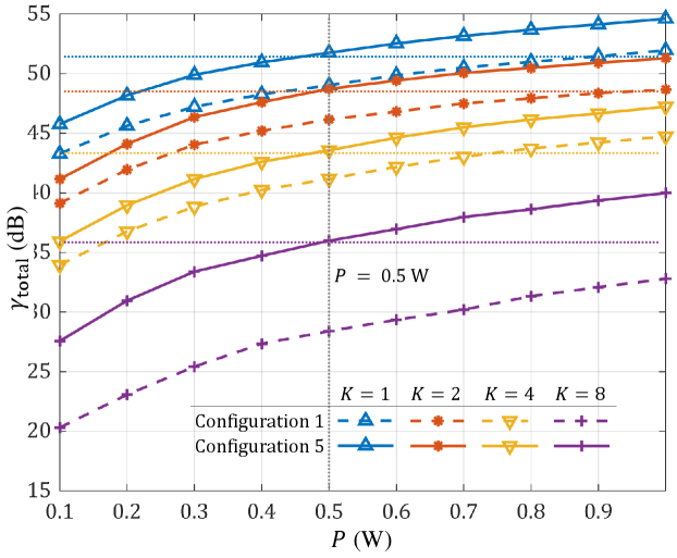
V-B3 Transmit power reduction and convergence behavior
Next, we examine how the equivalent total SNR varies with the total transmit power . The simulation results are shown in Fig. 12 and explained as follows.
-
•
For a fixed number of users, increasing leads to a higher , whereas increasing the number of users results in a lower .
-
•
With polarization matching through rotations of both transmitting and receiving antennas, the PAMA framework demonstrates greater power efficiency. To achieve the same total SNR, PAMA significantly reduces the required transmit power. This outcome aligns with expectations, as the transmitter can adjust its orientation to direct higher field intensity toward each user, while the receiver can optimize matching efficiency by rotating its antenna for optimal alignment.
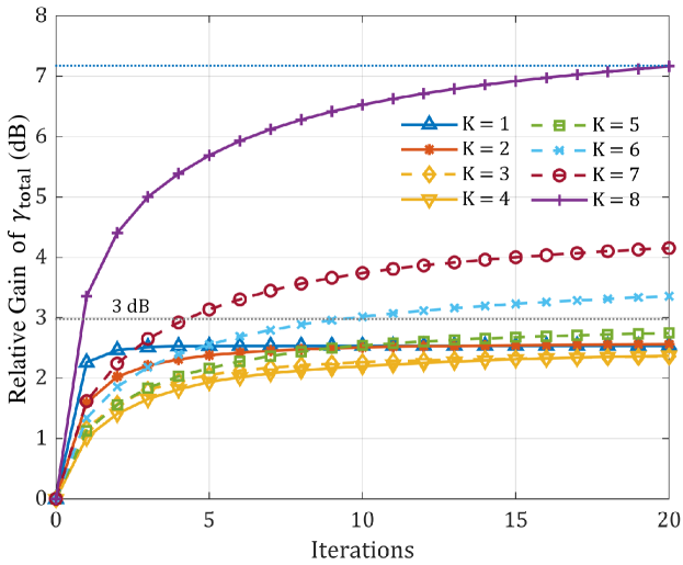
Finally, Fig. 13 illustrates the convergence behavior of our optimization algorithm by showing the relative gain in total SNR. The results reveal that:
-
•
The total SNR increases with each iteration across various values of . For , the algorithm typically converges within about iterations, achieving a gain of less than dB. However, when , more iterations are required for convergence.
-
•
Despite the increased number of iterations needed for larger , the additional receiving antennas introduce greater degrees of freedom, enabling higher gains within a reasonable number of iterations. For instance, with , the gain can reach up to dB within 20 iterations.
VI Conclusion
This paper presented the PAMA framework, which integrates polarization effects into the translation and rotation of antennas in wireless communication systems. By factoring in polarization, PAMA uncovers a defining advantage of MA: the ability to optimize polarization matching between the transmitter and receiver. This enhancement debunks the belief that MA is only effective in low-frequency multipath environments and extends the applicability of MA to higher frequency bands like the mmWave spectrum.
At mmWave frequencies, antennas are physically smaller, making them easier to move and rotate, which facilitates the practical implementation of PAMA systems. The dominance of LOS paths in the mmWave band simplifies channel estimation compared to traditional MA systems operating in environments with rich multipath. Additionally, PAMA achieves near-optimal performance with low rotation granularity. These factors collectively enhance the feasibility of deploying PAMA in real-world scenarios.
The insights from this work underscore the critical role of polarization in maximizing the performance of MA. Future research may focus on integrating PAMA with other advanced communication technologies, evaluating its performance in various high-frequency settings, and addressing practical implementation challenges such as antenna control mechanisms and mobility constraints. By advancing the understanding of how polarization can be harnessed in movable antenna systems, this work lays the foundation for developing more efficient and reliable wireless communication networks.
Appendix A Electric Field Radiation
As a preliminary, the appendix explains the derivation of (5), the radiation patterns of a half-wave dipole.
Maxwell’s equations can be written as
| (31) | |||
| (32) | |||
| (33) | |||
| (34) |
where
-
•
and refer to the electric field and magnetic field.
-
•
is the magnetic permeability of air, describing its ability to conduct magnetic field lines. is the permittivity, characterizing a material’s capacity to store electric charge.
-
•
and represent the source current density and source charge density, respectively.
-
•
is the angular frequency of the wave. The expression denotes the cross product; denotes the curl of ; denotes the dot product; denotes the divergence of , and is the Hamiltonian operator.
Since the divergence of in (34) is zero, the vector field has no sources or sinks; it only circulates. This allows us to define a magnetic vector potential so that can be described as the curl of :
| (35) |
Substituting (35) into (31) yields . In vector calculus, if the curl of a vector field is zero, that field can be expressed as the gradient of a scalar potential. Therefore, we can define an electric scalar potential such that
| (36) |
It is important to note that is always zero for any scalar potential .
Equations (35) and (36) show how and can be represented in terms of their potential functions. This means that once we find these potential functions, we can determine the corresponding field expressions. The next step is to solve for these potential functions.
First, substituting (35) into (32) gives
| (37) |
Next, we use the vector identity , where represents the Laplace operator, which calculates the divergence of the gradient. By applying (36), we can rewrite (37) as
| (38) |
After a simple rearrangement and using the Lorentz condition [21], we get
| (39) |
This equation is known as the vector wave equation. With this differential equation, if the current is known, we can solve for the vector potential . Once is determined, the magnetic field can be found using (35). Then, by using the Lorentz condition along with (36), the electric field can also be solved.
To solve for , we break down the vector wave equation in (39) into three separate scalar equations. Substituting these into (39), we obtain
| (40) |
where is the phase constant of the transmitted wave, representing the phase change per unit distance.
The three equations in (A) are structurally the same. Once we solve one of them, the solutions for the other two follow easily. To start, we find the solution for a point source. This solution, known as the unit impulse response, can be used to build a general solution by considering an arbitrary source as a combination of many point sources. The differential equation for a point source is
| (41) |
where represents the response to a point source located at the origin, and is the unit impulse function. Although a point source is infinitesimally small, the current it represents has a specific direction. In practical problems, the point source models a small segment of current with a defined direction. If we consider the point source current to be directed along the -axis, then .
Since the point source only exists at the origin and is zero everywhere else, (41) can be simplified to
| (42) |
The two solutions to this equation are , where is the distance from the point source to the observation point . These solutions represent waves moving outward and inward from the source, respectively. The physically relevant solution is the one that describes waves propagating outward from the point source. By determining the constant of proportionality, the solution for the point source becomes
| (43) |
For a current density directed along the -axis, the resulting vector potential will also be -directed. If we think of the source as a collection of point sources with a distribution given by , the response can be found by summing the responses of each point source using (43). This summation is represented by an integral over the source volume :
| (44) |
Similar integrals apply for the - and -components. The overall solution is the sum of all components, expressed as
| (45) |
where is the vector from the location of the point source to the observation point , hence is given by . Therefore, we arrive at the solution to the vector wave equation (39) as shown in (45).
In summary, when the current density is known, the steps to find the induced field are:
For a half-wave dipole located at the origin and placed along the -axis, the current density distribution is given by
| (46) |
where .
The magnetic vector potential can be derived from (45) as follows:
| (47) | |||
where (a) follows from in the far field; (b) follows because the polar angle of the observation point is the emission angel of the transmitting antenna when the dipole is oriented along the -axis; (c) follows from (46); (d) follows from , , and , .
Finally, the electric field induced at can be derived as
| (48) | |||||
Appendix B Proof of Corollary 3
Since the first multiplicative factor in (9) is a constant, the behavior of the magnitude is determined by the second term: . We analyze the derivative of with respect to (w.r.t) to examine its variation.
The derivative can be expressed as
| (49) |
where . To simplify the notations, we define and .
When , we have
Thus, is a monotonically decreasing function of from 1 to . The minimum value of occurs at or . Since
we have for . Therefore, , and
On the other hand, we have
is a monotonically decreasing function when , with and . Therefore, , implying that , and thus
Additionally, when . Overall, we have when .
Similarly, it can be shown that when . Since , both and the magnitude reach their maximum when , proving the corollary.
References
- [1] S. Dang, O. Amin, B. Shihada, and M.-S. Alouini, “What should 6G be?” Nature Electronics, vol. 3, no. 1, pp. 20–29, 2020.
- [2] C.-X. Wang, X. You, X. Gao, X. Zhu, Z. Li, C. Zhang, H. Wang, Y. Huang, Y. Chen, H. Haas et al., “On the road to 6G: Visions, requirements, key technologies, and testbeds,” IEEE Communications Surveys & Tutorials, vol. 25, no. 2, pp. 905–974, 2023.
- [3] L. Zhu, W. Ma, and R. Zhang, “Modeling and performance analysis for movable antenna enabled wireless communications,” IEEE Transactions on Wireless Communications, 2023.
- [4] X. Shao, Q. Jiang, and R. Zhang, “6D movable antenna based on user distribution: Modeling and optimization,” arXiv preprint arXiv:2403.08123, 2024.
- [5] X. Shi, X. Shao, and R. Zhang, “Capacity maximization for base station with hybrid fixed and movable antennas,” arXiv preprint arXiv:2405.07176, 2024.
- [6] B. Ning, S. Yang, Y. Wu, P. Wang, W. Mei, C. Yuen, and E. Björnson, “Movable antenna-enhanced wireless communications: General architectures and implementation methods,” arXiv preprint arXiv:2407.15448, 2024.
- [7] K.-K. Wong, A. Shojaeifard, K.-F. Tong, and Y. Zhang, “Fluid antenna systems,” IEEE Transactions on Wireless Communications, vol. 20, no. 3, pp. 1950–1962, 2020.
- [8] K.-K. Wong and K.-F. Tong, “Fluid antenna multiple access,” IEEE Transactions on Wireless Communications, vol. 21, no. 7, pp. 4801–4815, 2021.
- [9] K.-K. Wong, K.-F. Tong, Y. Shen, Y. Chen, and Y. Zhang, “Bruce Lee-inspired fluid antenna system: Six research topics and the potentials for 6G,” Frontiers in Communications and Networks, vol. 3, pp. 853–416, 2022.
- [10] K. K. Wong, A. Shojaeifard, K.-F. Tong, and Y. Zhang, “Performance limits of fluid antenna systems,” IEEE Communications Letters, vol. 24, no. 11, pp. 2469–2472, 2020.
- [11] M. Khammassi, A. Kammoun, and M.-S. Alouini, “A new analytical approximation of the fluid antenna system channel,” IEEE Transactions on Wireless Communications, vol. 22, no. 12, pp. 8843–8858, 2023.
- [12] T. Yoo and A. Goldsmith, “On the optimality of multiantenna broadcast scheduling using zero-forcing beamforming,” IEEE Journal on Selected Areas in Communications, vol. 24, no. 3, pp. 528–541, 2006.
- [13] D. Tse and P. Viswanath, Fundamentals of wireless communication. Cambridge university press, 2005.
- [14] W. Tang, M. Z. Chen, X. Chen, J. Y. Dai, Y. Han, M. Di Renzo, Y. Zeng, S. Jin, Q. Cheng, and T. J. Cui, “Wireless communications with reconfigurable intelligent surface: Path loss modeling and experimental measurement,” IEEE Transactions on Wireless Communications, vol. 20, no. 1, pp. 421–439, 2020.
- [15] Q. Wu and R. Zhang, “Intelligent reflecting surface enhanced wireless network via joint active and passive beamforming,” IEEE Transactions on Wireless Communications, vol. 18, no. 11, pp. 5394–5409, 2019.
- [16] L. Zhu, W. Ma, B. Ning, and R. Zhang, “Movable-antenna enhanced multiuser communication via antenna position optimization,” IEEE Transactions on Wireless Communications, 2023.
- [17] W. Ma, L. Zhu, and R. Zhang, “MIMO capacity characterization for movable antenna systems,” IEEE Transactions on Wireless Communications, 2023.
- [18] C. Psomas, P. J. Smith, H. A. Suraweera, and I. Krikidis, “Continuous fluid antenna systems: Modeling and analysis,” IEEE Communications Letters, 2023.
- [19] W. L. Stutzman and G. A. Thiele, Antenna theory and design. John Wiley & Sons, 2012.
- [20] M. Costa, A. Richter, and V. Koivunen, “DoA and polarization estimation for arbitrary array configurations,” IEEE Transactions on Signal Processing, vol. 60, no. 5, pp. 2330–2343, 2012.
- [21] Y. Huang, Antennas: from theory to practice. John Wiley & Sons, 2021.
- [22] R. U. Nabar, H. Bolcskei, V. Erceg, D. Gesbert, and A. J. Paulraj, “Performance of multiantenna signaling techniques in the presence of polarization diversity,” IEEE Transactions on Signal Processing, vol. 50, no. 10, pp. 2553–2562, 2002.
- [23] M. Kurum, M. Deshpande, A. T. Joseph, P. E. O’Neill, R. H. Lang, and O. Eroglu, “SCoBi-Veg: A generalized bistatic scattering model of reflectometry from vegetation for signals of opportunity applications,” IEEE Transactions on Geoscience and Remote Sensing, vol. 57, no. 2, pp. 1049–1068, 2018.
- [24] Y. Niu, Y. Li, D. Jin, L. Su, and A. V. Vasilakos, “A survey of millimeter wave communications (mmWave) for 5G: opportunities and challenges,” Wireless networks, vol. 21, pp. 2657–2676, 2015.
- [25] R. W. Heath, N. Gonzalez-Prelcic, S. Rangan, W. Roh, and A. M. Sayeed, “An overview of signal processing techniques for millimeter wave MIMO systems,” IEEE Journal of Selected Topics in Signal Processing, vol. 10, no. 3, pp. 436–453, 2016.
- [26] Study on channel model for frequencies from 0.5 to 100 GHz (3GPP TR 38.901 version 18.0.0 Release 18), 3GPP Std. 3GPP TR 38.901, 2024.
- [27] J. A. Stratton, Electromagnetic theory. John Wiley & Sons, 2007, vol. 33.
- [28] C. Parazzoli, R. Greegor, K. Li, B. Koltenbah, and M. Tanielian, “Experimental verification and simulation of negative index of refraction using snell’s law,” Physical Review Letters, vol. 90, no. 10, p. 107401, 2003.
- [29] O. Tervo, L.-N. Tran, and M. Juntti, “Optimal energy-efficient transmit beamforming for multi-user MISO downlink,” IEEE Transactions on Signal Processing, vol. 63, no. 20, pp. 5574–5588, 2015.
- [30] W. Yu, W. Rhee, S. Boyd, and J. M. Cioffi, “Iterative water-filling for gaussian vector multiple-access channels,” IEEE Transactions on Information Theory, vol. 50, no. 1, pp. 145–152, 2004.
- [31] M. Sadek, A. Tarighat, and A. H. Sayed, “A leakage-based precoding scheme for downlink multi-user MIMO channels,” IEEE Transactions on Wireless Communications, vol. 6, no. 5, pp. 1711–1721, 2007.