Polariton Localization and Dispersion Properties of Disordered Quantum Emitters in Multimode Microcavities
Abstract
Experiments have demonstrated that the strong light-matter coupling in polaritonic microcavities significantly enhances transport. Motivated by these experiments, we have solved the disordered multimode Tavis-Cummings model in the thermodynamic limit and used this solution to analyze its dispersion and localization properties. The solution implies that wave-vector-resolved spectroscopic quantities can be described by single-mode models, but spatially resolved quantities require the multimode solution. Nondiagonal elements of the Green’s function decay exponentially with distance, which defines the coherence length. The coherence length is strongly correlated with the photon weight and exhibits inverse scaling with respect to the Rabi frequency and an unusual dependence on disorder. For energies away from the average molecular energy and above the confinement energy , the coherence length rapidly diverges such that it exceeds the photon resonance wavelength . The rapid divergence allows us to differentiate the localized and delocalized regimes and identify the transition from diffusive to ballistic transport.
pacs:
Introduction.— The spatial confinement of the light field in microcavities gives rise to dispersive polaritons with outstanding spectroscopic properties [1] and establishes an alternative channel for charge and energy transport different from the short-range hopping. Recent experimental measurements of microcavities have found that transport can be enhanced by orders of magnitude [2, 3, 4, 5, 6, 7]. A thorough description is challenging because of the large number of light modes in the cavity and the energetic, spatial and orientational disorder.
Many theoretical models describe the light field by a single cavity mode, which is coupled to a macroscopic number of quantum emitters [8, 9, 10, 11, 12, 13, 14, 15, 16, 17, 18, 19, 20, 21, 22, 23, 24, 25, 26, 27]. Recent investigations have predicted an intriguing turnover of the transport, relaxation and the linewidth as a function of disorder [9, 8]. However, due to the all-to-all coupling structure in single-mode models, excitons can travel instantaneously between distant emitters and thus exceed the speed of light, potentially leading to an unphysical prediction for the transport efficiency.
Since the photonic dispersion relation ensures the speed of light, the light fields should be described as a continuum of cavity modes. For example, the impact of disorder on polaritons was investigated perturbatively [28, 29, 30, 31]. Exact diagonalization and integration [32, 33], mean-field based approaches [34, 35, 36, 37], Monte-Carlo methods [38] and density-functional theory [39] have been used to numerically investigate multimode models. Yet, a fully microscopic and analytical solution of the light-matter dynamics for disordered quantum emitters is still lacking.
In this Letter, we analytically and numerically solve the multimode disordered Tavis-Cumming model nonperturbatively. Our closed-form solution predicts a finite coherence length for all polariton energies. Away from the average molecular energy , the coherence length rapidly diverges and exceeds by far the typical length of realistic microcavities. This defines two transport regimes in the energy spectrum: one regime of strongly localized polaritons, where transport is diffusive, and one regime of delocalized polaritons, where the large coherence length can support ballistic transport. The coherence length exhibits a turnover as a function of disorder, which has no analog in the Anderson localization [40, 41, 42], but is reminiscent of noise-assisted transport [43, 44].
Multimode disordered Tavis-Cummings model.— As shown in Figs. 1(a) and 1(b), we consider a one-dimensional microcavity of length which contains quantum emitters representing atoms, molecules, NV centers or particle-hole pairs in semiconductors. For concreteness, we focus on molecules in the following. We adopt a multimode disordered Tavis-Cummings model, whose Hamiltonian is given as where
| (1) |
The molecules are described by bosonic operators . Here, the excitation energies are distributed according to a Gaussian function with center and disorder width . Yet, our findings also hold for arbitrary disorder distributions. The light field is quantized by the photonic operators labeled by . The photonic dispersion relation is , where is the speed of light, is the wave vector (specified below), and is the confinement energy depending on the geometry of the microcavity. As the total excitation number is conserved, we can restrict our analysis to the single-excitation manifold. The light-matter interaction in Eq. (1) is given by where is the position of molecule , is the wave vector dependent light-matter interaction, and are the photonic mode functions in one-dimensional space. We restrict the current investigation to energetic disorder, while spatial and orientational disorder will be considered elsewhere later.
For the numerical calculations we use an open boundary condition, such that the photonic modes are for the wave vectors with integer [45]. In the analytical calculation, we assume a periodic boundary condition such that the photonic modes are , where with integer . We note that in the limit, the boundary condition has a negligible effect.
Analytical solution. The Heisenberg equations of and are transformed into the Laplace space defined by for arbitrary operators . We find that the coupling between different cavity modes scales as and thus vanishes in the thermodynamic limit with constant density [45]. In other words, one can treat the system as a superpostion of uncoupled single-mode systems, which have been investigated in detail in Refs. [9, 46, 47]. The solution of the Heisenberg operators in this limit is
| (2) | |||||
where and denote the initial conditions of the time evolution. We have defined the renormalized photon energy by
| (3) |
where the dependence reflects a retardation effect. We have expressed the disorder average in terms of the density and the disorder-averaged Green’s function of the unperturbed molecules . Using Eq. (2), we can construct arbitrary retarded Green’s functions such as or . Performing the disorder average, the Green’s function for reads as
| (4) |
These Green’s functions are equivalent to the single-mode system when the sum over is neglected. The simple superposition of all modes reflects the mode decoupling in the thermodynamic limit, for which the matter system becomes homogeneous in a statistical sense.
Spectroscopy.— The wave-vector-resolved photon and molecule local density of states (LDOSs) are given as with and , respectively, and can be measured spectroscopically [9].
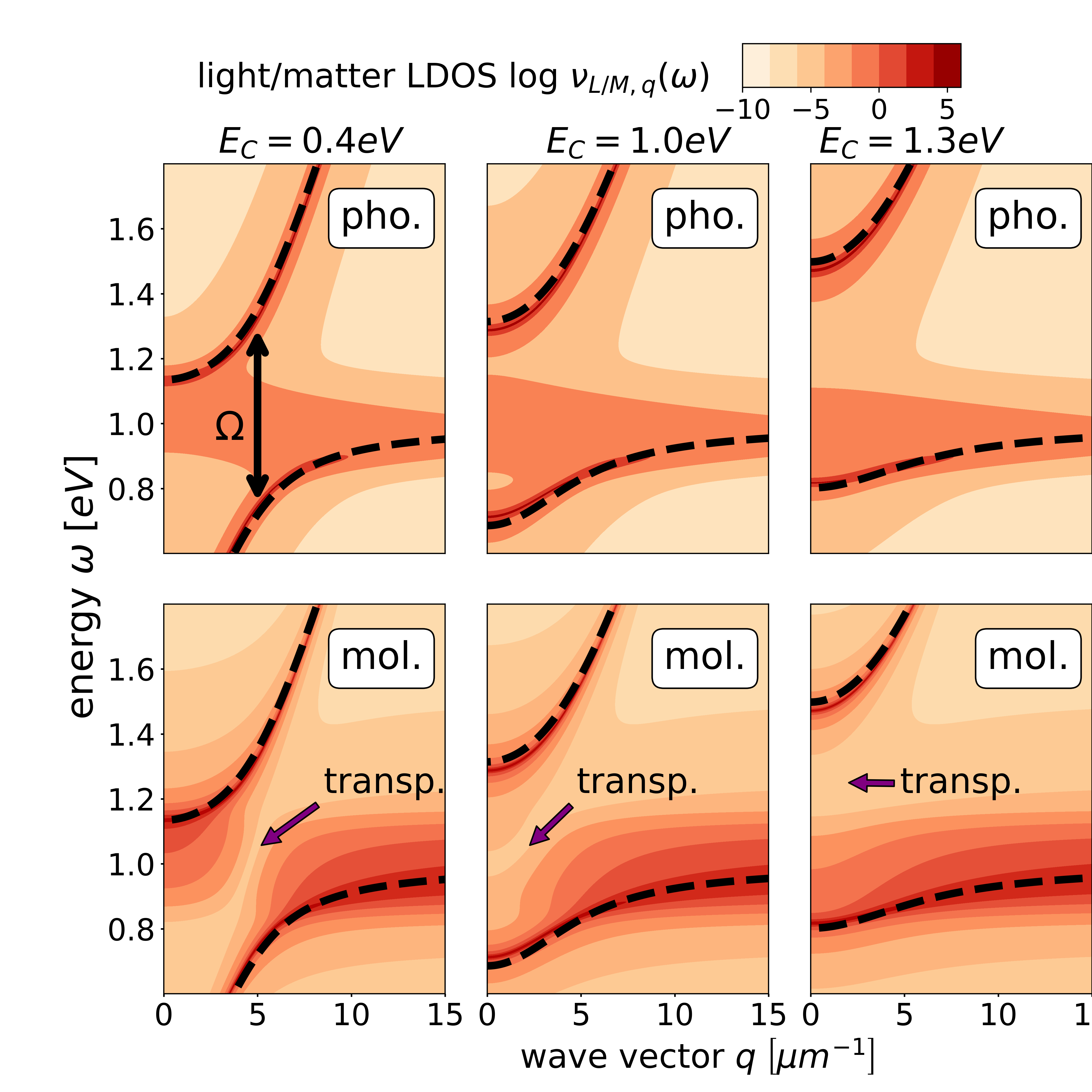
In Fig. 1(c), we investigate the LDOSs for . The LDOSs for and can be found in the Supplementary Materials [45]. The dashed lines depict the lower and upper polaritons for a vanishing disorder . Close to , where both dispersions would cross for , the lower and upper polaritons exhibit a Rabi splitting of . The photon and molecule LDOSs closely follow the photonic dispersion curves of the disorder-free systems (dashed). The photon LDOS accumulates close to the photon dispersion , but also around close to the polariton anticrossing, where light and matter are strongly mixed. The molecule LDOS accumulates around , where it resembles the original disorder distribution. Along and away from , the molecule LDOS is one order of magnitude smaller than the photon LDOS. Because of level repulsion, the molecule LDOS is suppressed for energies at the anticrossing (purple arrow), which resembles the electromagnetically induced transparency and related effects [48, 9, 49, 50]. As each photon mode interacts with a disordered ensemble, the level repulsion is smeared out in the photon LDOS.
The photon and molecule weights of a specific eigenstate with energy is given as , where , and is the photon (molecule) projection operator. The numerical calculation in Fig. 1 (d,e,f) verifies the analytical solution for various . (i) For , the photon weight vanishes around the resonance condition , as the molecules by far outnumber the photon modes in this energy region. The photon weight increases monotonically with increasing distance from the resonance condition. (ii) For , the photon weight does not monotonically increase with distance from . The peak around is a consequence of the polariton formation, causing the light field to be pushed down energetically. (iii) For , light and matter are energetically separated such that the mutual influence is rather weak. Motivated by Ref. [32], we define dark (bright) states as eigenstates with a photonic weight (), which accumulate in the dip of the photon weight in Fig. 1(d).
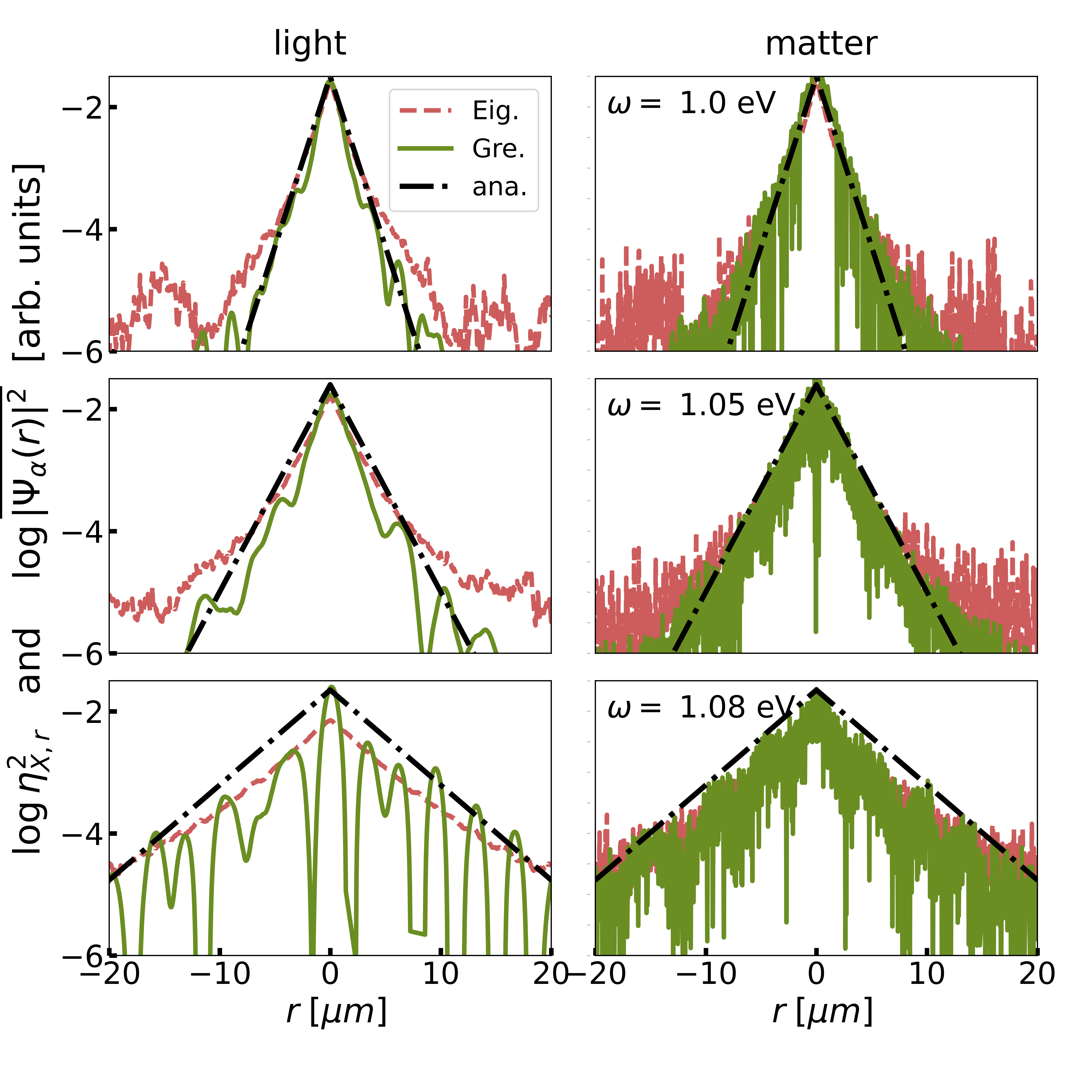
Polariton localization. Figure 2 (a) depicts the imaginary part of the Green’s function in position space,
| (5) |
where , for and three different energies . In this definition we have used the translational invariance of the Green’s function in the limit. The photon (molecule) Green’s function is depicted for (). Clearly, the amplitude of the Green’s function shows an exponential decay with increasing , where the coherence length depends on energy.
Figure 2(b) depicts the imaginary part of the Green’s function in wave vector space, i.e., for . Overall, we observe that the widths of the Green’s functions in position and wave vector space are related by the Heisenberg uncertainty principle. In contrast to the photon contribution, which converges to zero for large wave vectors , the molecule Green’s function converges to a finite value. This is reflected by strong spatial fluctuations of the molecule Green’s function in position space in Fig. 2(a), which are absent in the photon Green’s function.
From Eq. (4) we can determine the coherence length using functional analysis, which characterizes the localization of the polaritons [51, 45]: In the limit, we find
| (6) |
where and . Specifically, the Green’s function decays as , where is the largest value such that is analytic for all . has two types of non-analyticities, namely the roots of the denominator and the branch cuts along the imaginary axis due to the root in . As explained later, the branch cut has minor influence on , such that the coherence length is effectively determined by the root of , i.e.,
| (7) |
where is assumed for simplicity. Interestingly, the coherence length depends via the product (i.e., the Rabi frequency) on the light-matter coupling .
In Figs. 1(g)-1(i) we compare the analytical expression for with the numerical evaluation [45], which confirms the validity of the analytical solution. For large energies , we observe that the coherence length diverges. For realistic parameters and energies , the branch cuts starting at have a minor influence on the coherence length, as for a large , is significantly smaller than , while for small , the influence of the branch cut in the Fourier transformation in Eq. (6) is negligible and the Green’s function is still mainly determined by the pole of the Green’s function [45].
Analysis.— In Fig. 1 we demonstrate a correlation between the photon weight and the coherence length. As the interaction between the molecules is mediated via photons, the coherence length increases when photons can travel further without being scattered by molecules. The relation of coherence length and photon scattering can be understood by expanding the Green’s function in orders of , where destructive interference of distinct photon scattering paths decrease the coherence length for increasing [45]. A low scattering probability is reflected by a large photon weight in the Green’s function. The coherence length of the Green’s function can thus be identified with the absorption length for light traveling along the extended direction of the cavity according to Beer’s absorption law [45]. Dark states have a detrimental impact on the coherence length. In general, we find a clear relation of dark states with a localized Green’s function, and bright states with a delocalized Green’s function. The localized (delocalized) regimes are thereby described by (), where is the resonance wavelength of the molecular excitations.
In Fig. 3, we analyze the coherence length as a function of and for and . In Fig. 3(a) for small , we observe a clear linear dependence with slope for all energies . This can be explained by photon scattering, which consists of absorption () and reemission (). Interestingly, the coherence length for exhibits a dip for large , as the matter LDOS is strongly deformed and accumulates around , causing enhanced photon scattering.
The observations in Fig. 3(c) for and large are qualitatively similar to panel (a). The coherence length behaves very differently for small , where the photonic modes are absent for as . As for these energies eigenstates can be only formed with non-resonant photon modes, the coherence length for small is very small and almost independent of [45]. Interestingly, the coherence length increases over more than 1 order of magnitude for and because of the peak in the photon weight for small energies in Fig. 1(e).
Analyzing the coherence length as a function of disorder in Fig. 3(b), we observe a turnover as a function of . This is in contrast to the Anderson localization, where the coherence length monotonically decreases with disorder. Recent work has revealed a turnover of the steady-state flux as a function of disorder in the single-mode Tavis-Cummings model [9, 15, 8], which can be explained by the overlap of the photon LDOS and the molecule energy disorder distribution [9]. This interpretation can also be employed here. For small , the disorder distribution is strongly centered around . With increasing , the disorder distribution increases for , such that more molecules can resonantly scatter the photons with energy , which reduces the coherence length. For a large disorder, the molecule energies spread over a large energy regime, such that there are only few molecules in resonance with the photon modes close to , which enhances the coherence length. As the Gauss distribution becomes very flat close to the center for large , the coherence length becomes independent of for large . For , we do not observe a turnover, as the disorder distribution decreases monotonically for increasing . The turnovers can be also observed for in Fig. 3(d) for large , while overall the dependence on is more complicated because of the significant influence of the square root dispersion relation of close to .
Conclusions.— We have analytically and numerically solved the multimode disordered Tavis-Cummings model and predict its dispersion and localization properties. (i) The analytical solution is built on the mode decoupling and statistical self-averaging and is exact in the thermodynamic limit. Based on the solution, wave-vector-resolved properties such as broadened spectral line shape and dispersion can be predicted effectively within the single-mode treatment, whereas spatial-dependent properties such as transport and coherence length involve a wave vector summation and thus require the multimode formalism. (ii) A coherence length is introduced to characterize the finite size of the eigenstates as a function of the excitation energy and shows transitions from localized states around the molecular energy () to delocalized states away from . These transitions are strongly correlated with the photon weight and define a ballistic and a localized transport regime. (iii) Intriguingly, the coherence length is inversely proportional to the square of the Rabi frequency and can exhibit a turnover as a function of disorder. (iv) Both the dispersion and coherence length depend strongly on the cavity confinement energy : the number of available resonant photon modes and thus the light-matter coupling regime increase as the cavity changes from blueshifted (), resonance (), to redshifted (). The current investigation focuses on the one-dimensional system with energetic disorder, while higher-dimensional systems with spatial and orientational disorder will be considered elsewhere.
The coherence length crucially depends on the light-matter coupling and the disorder. For example, it can be enhanced by more than one order of magnitude with a slight increase of the light-matter interaction [cf. Fig. 3(c)]. Moreover, it can exhibit a turnover as a function of disorder, which contrasts the monotonically decreasing coherence length known from the Anderson localization, but is reminiscent of noise-assisted quantum transport [52, 53, 54, 55]. Arising from the overlap of the light LDOS and the disorder distribution, this turnover is induced by the same mechanism as the transport turnover previously predicted in the single-mode disordered Tavis-Cummings model [9]. Experimentally, this turnover can be investigated using a mixture of two molecular ensembles as in [18].
Noteworthy, the experiment in Ref. [7] has identified a transition from diffusive transport for small photonic weight to ballistic transport for large photonic weight. This observation is in perfect agreement with our analytical calculation, which predicts localized (i.e., diffusive) and delocalized (i.e., ballistic) eigenstates and a sharp transition as a function of excitation energy, as shown in Fig. 1. Theses findings reveal that the photonic weight explains the enhanced transport efficiency. In general, dark states with low photon weight correspond to localized states, while bright states with high photon weight correspond to delocalized states.
The experiment in Ref. [38] indicates that phonon-assisted coupling of diffusive eigenstates and ballistic eigenstates helps to overcome the localization. Extending our current model in Eq. (1) to incorporate phonon modes will quantitatively demonstrate this mechanism.
Moreover, as experimentally shown in [56], the detrimental impact of the cavity quality on transport properties can be modeled by a complex dispersion relation with . This will result in a complex energy shift in the coherence length in Eq. (7), leading to a suppression of transport. These and other experimental implications will be studied in future works.
G. E. gratefully acknowledges financial support from the Guangdong Provincial Key Laboratory of Quantum Science and Engineering (Grant No.2019B121203002); J. C. acknowledges support from the NSF (Grants No. CHE 1800301 and No. CHE1836913), the MIT sloan fund, and the Maria Curie FRIAS COFUND Fellowship Programme (FCFP) during his sabbatical in Germany.
References
- Garcia-Vidal et al. [2021] F. J. Garcia-Vidal, C. Ciuti, and T. W. Ebbesen, Manipulating matter by strong coupling to vacuum fields, Science 373, 0336 (2021).
- Lerario et al. [2017] G. Lerario, D. Ballarini, A. Fieramosca, A. Cannavale, A. Genco, F. Mangione, S. Gambino, L. Dominici, M. De Giorgi, G. Gigli, and D. Sanvitto, High-speed flow of interacting organic polaritons, Light: Sci. Appl. 6, e16212 (2017).
- Orgiu et al. [2015] E. Orgiu, J. George, J. A. Hutchison, E. Devaux, J. F. Dayen, B. Doudin, F. Stellacci, C. Genet, J. Schachenmayer, C. Genes, G. Pupillo, P. Samorì, and T. W. Ebbesen, Conductivity in organic semiconductors hybridized with the vacuum field, Nat. Mater. 14, 1123 (2015).
- Rozenman et al. [2018] G. G. Rozenman, K. Akulov, A. Golombek, and T. Schwartz, Long-range transport of organic exciton-polaritons revealed by ultrafast microscopy, ACS Photonics 5, 105 (2018).
- Hou et al. [2020] S. Hou, M. Khatoniar, K. Ding, Y. Qu, A. Napolov, V. M. Menon, and S. R. Forrest, Ultralong-range energy transport in a disordered organic semiconductor at room temperature via coherent exciton-polariton propagation, Adv. Mater. 32, 2002127 (2020).
- Krainova et al. [2020] N. Krainova, A. J. Grede, D. Tsokkou, N. Banerji, and N. C. Giebink, Polaron Photoconductivity in the Weak and Strong Light-Matter Coupling Regime, Phys. Rev. Lett. 124, 177401 (2020).
- Balasubrahmaniyam et al. [2023] M. Balasubrahmaniyam, A. Simkhovich, A. Golombek, G. Sandik, G. Ankonina, and T. Schwartz, From enhanced diffusion to ultrafast ballistic motion of hybrid light-matter excitations, Nat. Mater. 22, 338 (2023).
- Chávez et al. [2021] N. C. Chávez, F. Mattiotti, J. A. Méndez-Bermúdez, F. Borgonovi, and G. L. Celardo, Disorder-Enhanced and Disorder-Independent Transport with Long-Range Hopping: Application to Molecular Chains in Optical Cavities, Phys. Rev. Lett. 126, 153201 (2021).
- Engelhardt and Cao [2022] G. Engelhardt and J. Cao, Unusual dynamical properties of disordered polaritons in microcavities, Phys. Rev. B 105, 064205 (2022).
- Feist and Garcia-Vidal [2015] J. Feist and F. J. Garcia-Vidal, Extraordinary Exciton Conductance Induced by Strong Coupling, Phys. Rev. Lett. 114, 196402 (2015).
- Sommer et al. [2021] C. Sommer, M. Reitz, F. Mineo, and C. Genes, Molecular polaritonics in dense mesoscopic disordered ensembles, Phys. Rev. Res. 3, 033141 (2021).
- Spano [2015] F. C. Spano, Optical microcavities enhance the exciton coherence length and eliminate vibronic coupling in J-aggregates, J. Chem. Phys. 142, 184707 (2015).
- Shammah et al. [2017] N. Shammah, N. Lambert, F. Nori, and S. De Liberato, Superradiance with local phase-breaking effects, Phys. Rev. A 96, 023863 (2017).
- Botzung et al. [2020] T. Botzung, D. Hagenmüller, S. Schütz, J. Dubail, G. Pupillo, and J. Schachenmayer, Dark state semilocalization of quantum emitters in a cavity, Phys. Rev. B 102, 144202 (2020).
- Dubail et al. [2022] J. Dubail, T. Botzung, J. Schachenmayer, G. Pupillo, and D. Hagenmüller, Large random arrowhead matrices: Multifractality, semilocalization, and protected transport in disordered quantum spins coupled to a cavity, Phys. Rev. A 105, 023714 (2022).
- Zhang and Zhang [2021] Q. Zhang and K. Zhang, Collective effects of organic molecules based on the Holstein–Tavis–Cummings model, J. Phys. B 54, 145101 (2021).
- Gera and Sebastian [2022] T. Gera and K. L. Sebastian, Exact results for the Tavis-Cummings and Hückel Hamiltonians with diagonal disorder, J. Phys. Chem. A 126, 5449 (2022).
- Cohn et al. [2022] B. Cohn, S. Sufrin, A. Basu, and L. Chuntonov, Vibrational polaritons in disordered molecular ensembles, J. Phys. Chem. Lett. 13, 8369 (2022).
- Herrera and Spano [2016] F. Herrera and F. C. Spano, Cavity-Controlled Chemistry in Molecular Ensembles, Phys. Rev. Lett. 116, 238301 (2016).
- Houdré et al. [1996] R. Houdré, R. P. Stanley, and M. Ilegems, Vacuum-field Rabi splitting in the presence of inhomogeneous broadening: Resolution of a homogeneous linewidth in an inhomogeneously broadened system, Phys. Rev. A 53, 2711 (1996).
- Xiang et al. [2019] B. Xiang, R. F. Ribeiro, L. Chen, J. Wang, M. Du, J. Yuen-Zhou, and W. Xiong, State-selective polariton to dark state relaxation dynamics, J. Phys. Chem. A 123, 5918 (2019).
- Reitz et al. [2018] M. Reitz, F. Mineo, and C. Genes, Energy transfer and correlations in cavity-embedded donor-acceptor configurations, Sci. Rep. 8, 9050 (2018).
- Schäfer et al. [2019] C. Schäfer, M. Ruggenthaler, H. Appel, and A. Rubio, Modification of excitation and charge transfer in cavity quantum-electrodynamical chemistry, Proc. Natl. Acad. Sci. U.S.A. 116, 4883 (2019).
- Cao [2022] J. Cao, Generalized resonance energy transfer theory: Applications to vibrational energy flow in optical cavities, J. Phys. Chem. Lett. 13, 10943 (2022).
- Cui and Nitzan [2022] B. Cui and A. Nitzan, Collective response in light-matter interactions: The interplay between strong coupling and local dynamics, J. Chem. Phys. 157, 114108 (2022).
- Finkelstein-Shapiro et al. [2023] D. Finkelstein-Shapiro, P.-A. Mante, S. Balci, D. Zigmantas, and T. Pullerits, Non-Hermitian Hamiltonians for linear and nonlinear optical response: A model for plexcitons, J. Chem. Phys. 158, 104104 (2023).
- Zhang et al. [2023] Z. Zhang, X. Nie, D. Lei, and S. Mukamel, Multidimensional Coherent Spectroscopy of Molecular Polaritons: Langevin Approach, Phys. Rev. Lett. 130, 103001 (2023).
- Izrailev et al. [1998] F. M. Izrailev, S. Ruffo, and L. Tessieri, Classical representation of the one-dimensional Anderson model, J. Phys. A 31, 5263 (1998).
- Agranovich et al. [2003] V. M. Agranovich, M. Litinskaia, and D. G. Lidzey, Cavity polaritons in microcavities containing disordered organic semiconductors, Phys. Rev. B 67, 085311 (2003).
- Litinskaya and Reineker [2006] M. Litinskaya and P. Reineker, Loss of coherence of exciton polaritons in inhomogeneous organic microcavities, Phys. Rev. B 74, 165320 (2006).
- Litinskaya et al. [2004] M. Litinskaya, P. Reineker, and V. Agranovich, Fast polariton relaxation in strongly coupled organic microcavities, J. Lumin. 110, 364 (2004).
- Ribeiro [2022] R. F. Ribeiro, Multimode polariton effects on molecular energy transport and spectral fluctuations, Comm. Chem. 5, 48 (2022).
- Allard and Weick [2022] T. F. Allard and G. Weick, Disorder-enhanced transport in a chain of lossy dipoles strongly coupled to cavity photons, Phys. Rev. B 106, 245424 (2022).
- [34] J. Patton, V. Norman, R. Scalettar, and M. Radulaski, All-photonic quantum simulators with spectrally disordered emitters, arXiv:2112.15469.
- Ćwik et al. [2014] J. A. Ćwik, S. Reja, P. B. Littlewood, and J. Keeling, Polariton condensation with saturable molecules dressed by vibrational modes, Europhys. Lett. 105, 47009 (2014).
- Strashko et al. [2018] A. Strashko, P. Kirton, and J. Keeling, Organic Polariton Lasing and the Weak to Strong Coupling Crossover, Phys. Rev. Lett. 121, 193601 (2018).
- [37] I. Sokolovskii, R. H. Tichauer, J. Feist, and G. Groenhof, Enhanced excitation energy transfer under strong light-matter coupling: Insights from multi-scale molecular dynamics simulations, arXiv:2209.07309 .
- [38] D. Xu, A. Mandal, J. M. Baxter, S. W. Cheng, I. Lee, H. Su, S. Liu, D. R. Reichman, and M. Delor, Ultrafast imaging of coherent polariton propagation and interactions, arXiv:2205.01176.
- Alvertis et al. [2020] A. M. Alvertis, R. Pandya, C. Quarti, L. Legrand, T. Barisien, B. Monserrat, A. J. Musser, A. Rao, A. W. Chin, and D. Beljonne, First principles modeling of exciton-polaritons in polydiacetylene chains, J. Chem. Phys. 153, 084103 (2020).
- Anderson [1958] P. W. Anderson, Absence of diffusion in certain random lattices, Phys. Rev. 109, 1492 (1958).
- Abrahams et al. [1979] E. Abrahams, P. W. Anderson, D. C. Licciardello, and T. V. Ramakrishnan, Scaling Theory of Localization: Absence of Quantum Diffusion in Two Dimensions, Phys. Rev. Lett. 42, 673 (1979).
- Wang et al. [2020] Y. Wang, X. Xia, L. Zhang, H. Yao, S. Chen, J. You, Q. Zhou, and X.-J. Liu, One-Dimensional Quasiperiodic Mosaic Lattice with Exact Mobility Edges, Phys. Rev. Lett. 125, 196604 (2020).
- Cao and Silbey [2009] J. Cao and R. J. Silbey, Optimization of exciton trapping in energy transfer processes, J. Phys. Chem. A 113, 13825 (2009).
- Chuang et al. [2016] C. Chuang, C. K. Lee, J. M. Moix, J. Knoester, and J. Cao, Quantum Diffusion on Molecular Tubes: Universal Scaling of the 1D to 2D Transition, Phys. Rev. Lett. 116, 196803 (2016).
- [45] See Supplementary Material for more information about the solution of the TC model and the numerical calculations.
- Engelhardt et al. [2016] G. Engelhardt, G. Schaller, and T. Brandes, Bosonic Josephson effect in the Fano-Anderson model, Phys. Rev. A 94, 013608 (2016).
- Topp et al. [2015] G. E. Topp, G. Schaller, and T. Brandes, Steady-state thermodynamics of non-interacting transport beyond weak coupling, Europhys. Lett. 110, 67003 (2015).
- Fleischhauer et al. [2005] M. Fleischhauer, A. Imamoglu, and J. P. Marangos, Electromagnetically induced transparency: Optics in coherent media, Rev. Mod. Phys. 77, 633 (2005).
- Engelhardt and Cao [2021] G. Engelhardt and J. Cao, Dynamical Symmetries and Symmetry-Protected Selection Rules in Periodically Driven Quantum Systems, Phys. Rev. Lett. 126, 090601 (2021).
- Herrera and Litinskaya [2022] F. Herrera and M. Litinskaya, Disordered ensembles of strongly coupled single-molecule plasmonic picocavities as nonlinear optical metamaterials, J. Chem. Phys. 156, 114702 (2022).
- Reed and Barry [1975] M. Reed and S. Barry, Methods of Modern Mathematical Physics. II. Fourier Analysis, Self-Adjointness. (Academic Press, New-York-London, 1975) Section IX.3; Theorem IX.13.
- Wu et al. [2013] J. Wu, R. J. Silbey, and J. Cao, Generic Mechanism of Optimal Energy Transfer Efficiency: A Scaling Theory of the Mean First-Passage Time in Exciton Systems, Phys. Rev. Lett. 110, 200402 (2013).
- Lee et al. [2015] C. K. Lee, J. Moix, and J. Cao, Coherent quantum transport in disordered systems: A unified polaron treatment of hopping and band-like transport, J. Chem. Phys. 142, 164103 (2015).
- Engelhardt and Cao [2019] G. Engelhardt and J. Cao, Tuning the Aharonov-Bohm effect with dephasing in nonequilibrium transport, Phys. Rev. B 99, 075436 (2019).
- Chenu and Cao [2017] A. Chenu and J. Cao, Construction of Multichromophoric Spectra from Monomer Data: Applications to Resonant Energy Transfer, Phys. Rev. Lett. 118, 013001 (2017).
- Pandya et al. [2022] R. Pandya, A. Ashoka, K. Georgiou, J. Sung, R. Jayaprakash, S. Renken, L. Gai, Z. Shen, A. Rao, and A. J. Musser, Tuning the coherent propagation of organic exciton-polaritons through dark state delocalization, Adv. Sci. 9, 2105569 (2022).
Supplementary Materials
I Analytical calculations
I.1 System
We model an ensemble of disordered quantum emitters in a microcavity by the multimode disordered Tavis-Cummings Hamiltonian
| (1) |
where
| (2) |
Here, and label the quantum emitters and the photonic modes , respectively, both fulfilling a bosonic commutation relation. The quantum emitters can represent atoms, molecules or particle-hole pairs. For concreteness, we specify to molecules in this work. The excitation energies of the molecules are distributed according to a probability distribution . In this work, we mainly consider a Gaussian distribution,
| (3) |
with center and width , but our findings are also valid for arbitrary disorder models. We consider a one-dimensional translational-invariant system of length with a periodic boundary condition. The molecules are located at positions . The photonic dispersion relation is given by
| (4) |
with and integer . The confinement energy appears because of the spatial confinement of the light field in the transversal direction of the microcavity. The photonic mode functions are given by . The light-matter coupling is parameterized by . As the excitation number is an integral of motion, we focus on the single-excitation manifold for simplicity. In this work, we derive a closed-form expression for the Green’s function of the multimode Tavis-Cummings model in the thermodynamic limit, that we define by for a constant molecule density .
I.2 No disorder
Without disorder , all molecule energies are equal and the Hamiltonian can be easily diagonalized. Transforming the molecule operators into the wave-vector space, , we find that the Hamiltonian is block diagonal in and reads as
| (5) |
where we have assumed a constant for simplicity. For each , the two energies correspond to the lower and upper polaritons and are given as
| (6) |
where we have defined the Rabi splitting of the disorder-free system . The dispersion relations of the lower and upper polariton branches are depicted in Figs. 1 - 3 by dashed lines. The corresponding eigenstates are
| (7) |
where
| (8) |
with the Heaviside function .
Crucially, all molecule operators are coupled to the photonic operators with the same wave vector. Thus, in contrast to single-mode models, there are no dark states in the system. However, for very large , the photonic energy by far exceeds the molecule excitation energy such that and . In this limit, the photon modes and molecule modes are nearly decoupled such that the molecule mode can be considered as dark. We follow the approach suggested in Ref. [32] and classify an eigenstate according to its photon weight as dark or bright. Without disorder, the photon and molecule weights of the lower polariton are defined by
| (9) |
Accordingly, one can define the weights for the upper polariton. As suggested by Ref. [32], an eigenstate is classified as dark, when its photon weight is below a threshold value. In this work, we adopt the threshold value . For disordered systems, a general definition of the photon and molecule weights is given in Eq. (30).
I.3 Heisenberg equations of motion
The analytical solution for the system operators and can be obtained in Laplace space. This solution can then be used to construct arbitrary Green’s functions. The Heisenberg equations for the operators in the multimode Tavis-Cummings model read as
| (10) |
Transforming into the Laplace space defined by for arbitrary operators , the equations of motions become
| (11) |
where and denote the initial conditions of the operators at time . In general, this set of coupled linear equations can not be solved analytically for a large number of photonic modes. However, we can find an exact solution in the thermodynamic limit. To see this, we first resolve Eq. (I.3) and obtain
| (12) |
Inserting this into Eq. (11) and resolving for , we find
| (13) | |||||
where we have defined
| (14) | |||||
where will be denoted as self-energy. The third term in Eq. (13) represents an all-to-all coupling of the photonic modes, which cannot be solved in general. Fortunately, this term vanishes in the thermodynamic limit , as we explain in the following. To this end, we consider the factors
| (15) | |||||
In the second equality, we have inserted the parameterization . In the third line, we have introduced as a typical measure for . To explain the scaling of , we have excluded the cavity length normalizing the photonic mode functions .
Because of the energetic disorder, the real and imaginary parts and are samples of random variables and , respectively. According to the Gaussian law of large numbers, the means and the variances of the accumulated random variables scale as
| (16) |
Thus, the expectation values vanish except for , while the variances scale linearly with . Consequently, for we find . Thus, when approaching the thermodynamic limit while keeping the density constant, the terms with vanish.
I.4 Green’s function
Based on Eq. (17), one can directly obtain the retarded Green’s functions defined by
| (18) |
for photonic operators and molecule operators, respectively. As we consider bosonic operators in a non-interacting system, the expectation value in Eq. (18) does not depend on the initial condition, which we do not specify for this reason. Explicitly, the photonic and molecule Green’s functions read as
| (19) | |||||
Similarly, mixed light-matter Green’s functions can be constructed. Using the photonic mode functions, we can express the photon Green’s function in position space as
| (20) |
I.5 Disorder average
We define the disorder-averaged Green’s function as
| (21) |
where , and can label position or wave vector .
I.5.1 Self-energy
We observe that the photonic Green’s function in Eq. (19) depends on the disorder via the self energy in the renormalized frequencies in Eq. (14). Using , the self-energy becomes
| (22) | |||||
As the summation in the first line does not depend on the position, the sum over can be interpreted as an integral over the energy weighted by the disorder distribution for . Finally, we have introduced the disorder-averaged Green’s function of the uncoupled molecules
| (23) |
The key point in this derivation is that the self-energy term is self-averaging in the thermodynamic limit and thus does not require the external averaging operations defined in Eq. (21).
I.5.2 Disorder-averaged Green’s function
Given that the self energy is self averaging, it is now straight forward to perform the disorder average of the Green’s function in Eq. (19). Apart from , the photon Green’s function does not depend on the molecule energies such that the disorder-averaged Green’s functions coincides with the expressions in Eqs. (19) and (20) in position and wave vector space, respectively.
The disorder average of the matter function has the effect that the terms are replaced by in Eq. (23), i.e.,
| (24) | |||||
which in momentum space becomes
| (25) |
We emphasize that these Green’s functions are exact in the thermodynamic limit because of the self-averaging property of the self energy. Formally, the self average is equivalent to the celebrated coherent potential approximation (CPA). However, we emphasize that the CPA is exact for arbitrary disorder distributions for the model considered here. This is in contrast to nearest-neighbor and other short-range hopping models, where the CPA is only exact for the Lorentzian disorder model [55].
Noteworthy, the Green’s function in wave vector space in Eq. (19) and in Eq. (25) are identical to the Green’s function of the single-mode Tavis-Cummings model when replacing the photonic dispersion relation by the energy of the single cavity mode . The single-mode model with Lorentzian disorder has been investigated in detail in Ref. [9]. This shows that spectroscopic quantities, which can be wave-vector-resolved measured, can be correctly calculated using single-mode models. In contrast, the Greens’s functions in positions space given in Eq. (20) and (24) involve a summation of the wave vector. Therefore, we conclude that transport quantities and the coherence length cannot be accurately investigated in single-mode models. Thereby, the wave-vector summation in Eq. (20) and (24) ensures that the speed-of light is maintained as an upper bound in the dynamics.
I.6 Photon and molecule local density of states
In terms of the eigenstates and energies of the Hamiltonian in Eq. (1), we define the wave-vector-resolved photon and molecule local density of states (LDOS) via
| (26) |
with an infinitesimal . We note that the photon and molecule LDOS can be measured by angular-resolved spectroscopy. The diagonal elements of the Green’s function in Eq. (18) can be formally written as
| (27) |
where and are the eigenstates in wave vector representation. Using the Dirac identity , it is now straightforward to show that
| (28) |
for . For later purpose, we also define the total density of states
| (29) | |||||
where is the number of eigenstates in the energy interval having an infinitesimal width . The equality in the second line follows from the fact that in the single-excitation manifold.
In Fig. 1, we analyze the photon and molecule LDOSs for three confinement energies , and . For simplicity we assume a wave-vector-independent light-matter interaction . All three photon and molecule LDOSs look qualitatively similar. Yet, we find that the photon LDOS for has a significant smaller contribution for energies close to than the ones for and . In contrast, the matter LDOS for has a significant smaller contribution close to the photon dispersion than the ones for and .
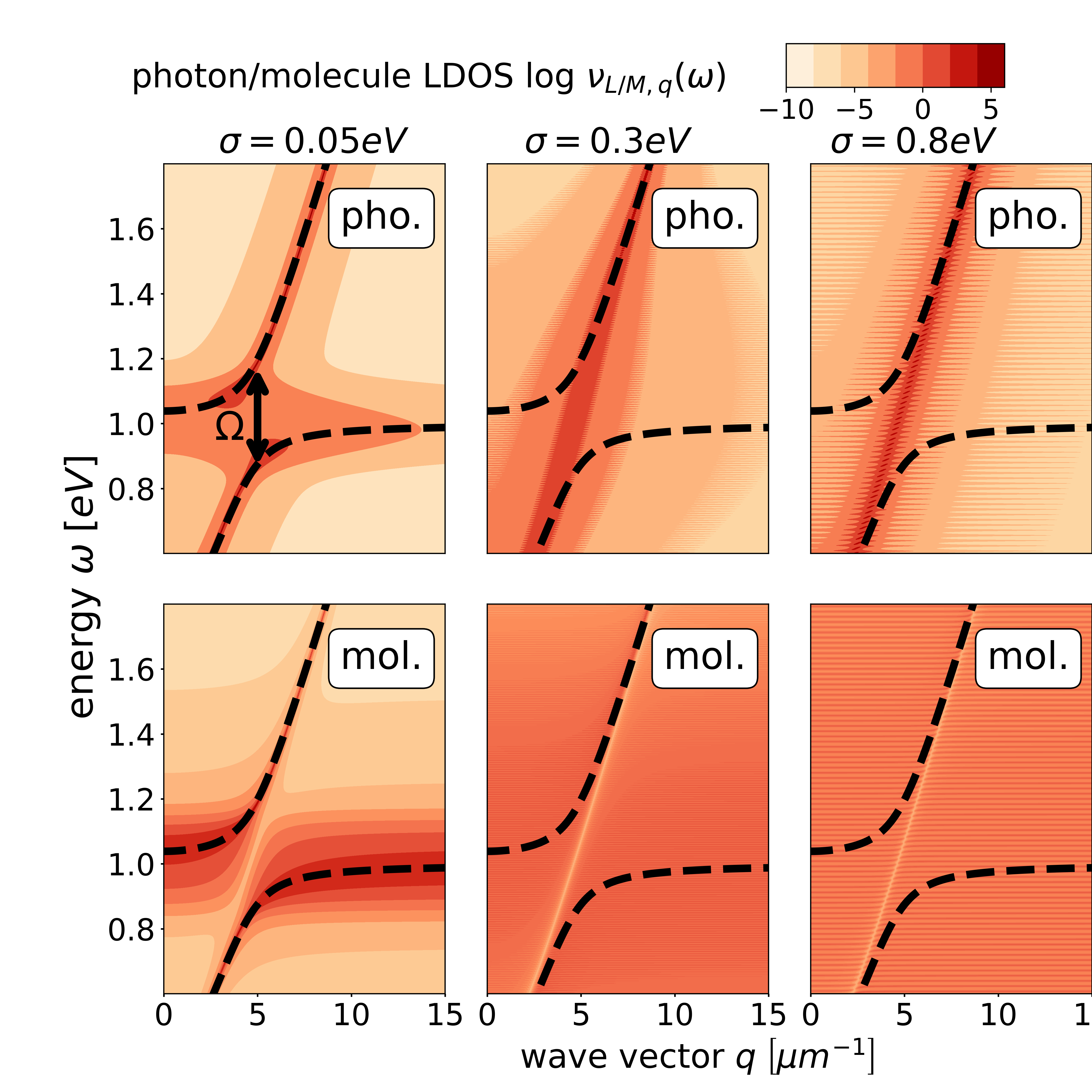
In Fig. 2, we analyze the LDOSs for the same parameters as in Fig. 1, but for a larger light-matter coupling. Accordingly, we see that now the Rabi splitting is significantly larger. Consequently, the transparency effect in the matter LDOS within the gap is better visible.
Next, we investigate the influence of disorder on the photon and molecule LDOSs, which is depicted in Fig. 3 for three different . For , we observe two separate polariton bands, that merge for . When further increasing to , the photon LDOS increasingly concentrates around the photon dispersion relation : for increasing , the molecular excitation energies are distributed over a larger energy range, which leads to an increasing decoupling of photonic and molecular systems, analog to the behavior in single-mode models [9].
I.7 Photon and molecule weights
The photon and molecule weights of a polariton determine its dynamical properties. In terms of the eigenstates of the multimode Tavis-Cummings Hamiltonian, these quantities are defined as
| (30) |
where . In the numerical calculations, we evaluate the averaged quantities
| (31) |
where is the number of eigenstates in the energy interval of width . Note that due to their definition, the photon and matter weights sum up to one, i.e., . Using the definitions of the wave-vector-resolved LDOS in Eq. (26) and the total density of states in Eq. (29), we find
| (32) |
Thus, the photon (molecule) weight is the photon (molecule) LDOS integrated over the wave vector and normalized by the total density of states. This expression can be numerically integrated using the analytical expression of the Greens’s functions in Eq. (19) and (25).
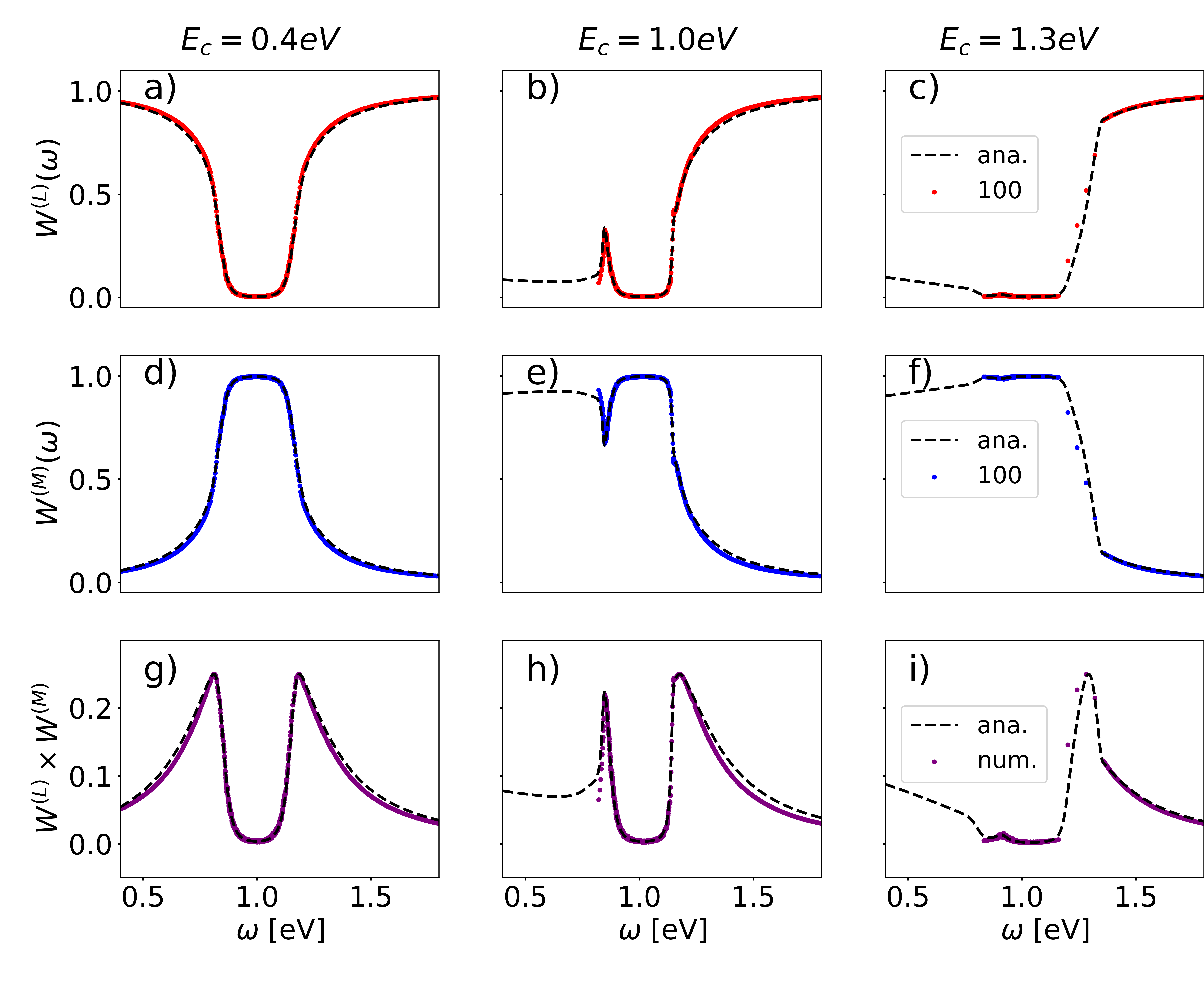
In Fig. 4 (a) - (c) we depict the photon weight as a function of energy for three different confinement energies . These plots serve also as a benchmark calculation of our analytical solution in Eqs. (19) and (25). Thereby, the weights have been numerically evaluated using Eq. (31), where the eigenstates have been obtained by numerical diagonalization of the Hamiltonian. In panels (a)- (c) we observe a significant dip in the photon weight for energies around . As the photon weight is less than , these eigenstates are classified as dark states according to the explanations in Sec. I.2. In panel (b) and (c) we find that the photon weight is larger than only for energies above , as the photonic dispersion relation is bounded by from below. The panels Fig. 4 (d) - (f) depict the corresponding matter weights. Moreover, we depict the light-matter mixing, which we define as the product . The peaks of this quantity clearly resembles the lower and upper polariton bands.
I.8 Asymptotic behavior in position space
Next, we are interested in the asymptotic behavior of the Green’s function in position space, i.e., we investigate for and large , where with infinitesimal . From Eqs. (19) and (20) we see that the molecule Green’s function is proportional to the photon Green’s function when changes only slowly with . We thus continue to investigate the latter. In the continuum limit , the photon Green’s function in position space [c.f., Eq. (20)] reads as
where we can replace as the poles of the Green’s function are not located on the real axes because of the complex-valued .
We can analyze the asymptotic behavior of the Green’s function using a theorem of functional analysis [51]:
Let be in (space of square-integrable functions). Then for all if and only if its Fourier transformation has an analytic continuation to the set with the property that for each with , and for any : .
Applied to the Fourier transformation in Eq. (LABEL:eq:photonGreensFunctionContLim), this theorem states that the asymptotic behavior of the Green’s function is determined by the poles and branch cuts of the integrand (i.e., the Green’s function in wave vector space), where is now interpreted as a complex variable.
For simplicity, we consider the case . In this case the integrand is nonanalytic at
| (34) |
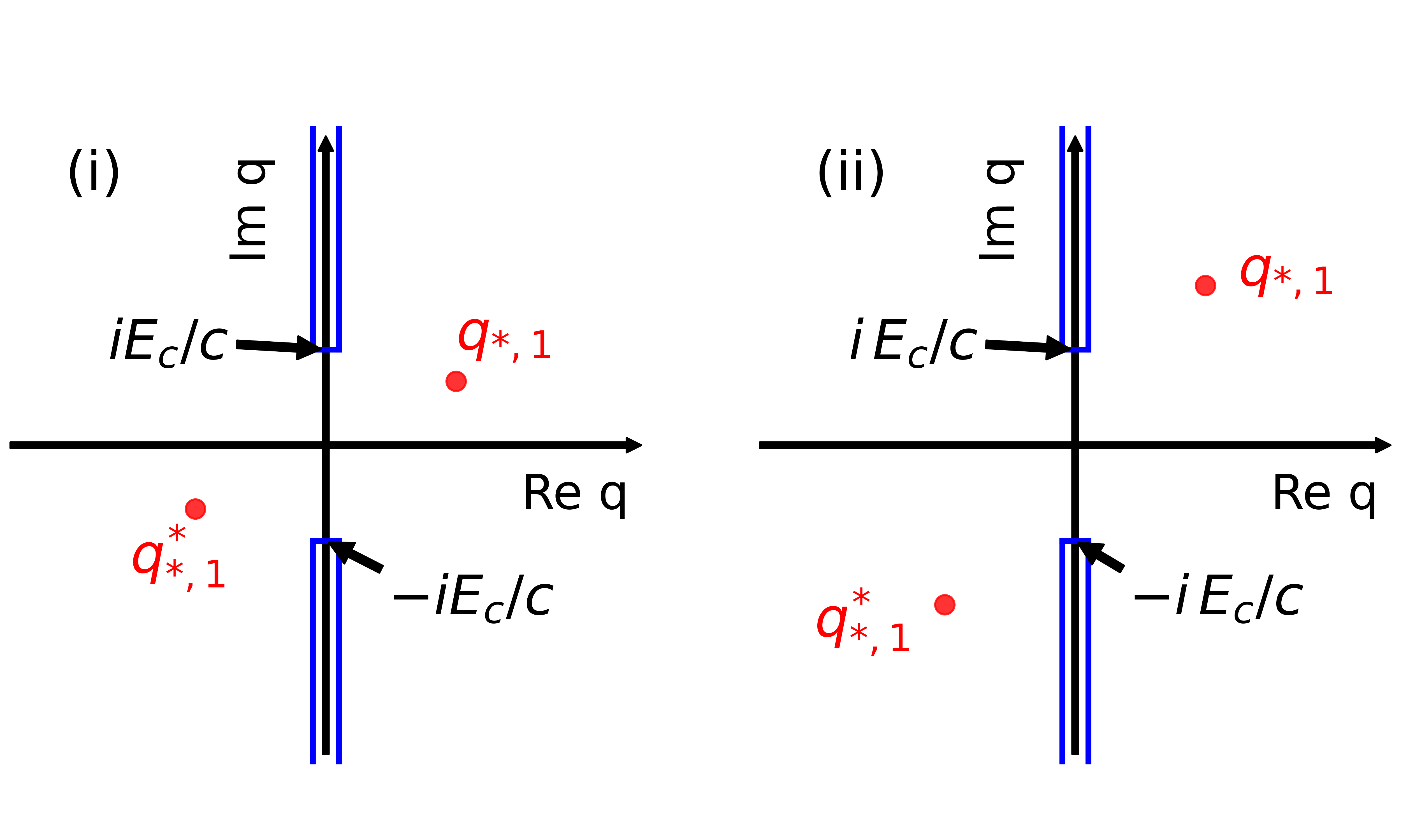
as well as the complex conjugate values. Thereby, appears because of the pole of the Green’s function , appears because of the branch cut induced by the photonic dispersion relation in Eq. (4). According to the above theorem, the asymptotic behavior is mainly determined by the nonanalyticity whose imaginary part is closer to zero.
In Fig. 5, we sketch two cases: (i) , and (ii) . In case (i), we find that the asymptotic decay is determined by the pole of the Green’s function. In this case, the coherence length depends on the light-matter interaction and other system parameters. In case (ii), the branch cut and, consequently, the ratio determines the asymptotic behavior. In short, the asymptotic behavior for large can be written as
| (35) |
where we have defined the coherence lengths
| (36) |
for . In the numerical calculations we find that the asymptotic behavior is accurately determined by , see Sec. II.2. For this reason, we assess that the coefficients fulfill , and we define the system’s coherence length as .
In the Letter, the coherence length for different values of the confinement energy is shown in Figs. 1(g)-(i). Comparing with the photon weight, we observe a clear correlation between both quantities, that will be explained in the next section. Consequently, the coherence length is very short in the energy range close to , that exhibits dark states. From this observation we conclude that dark states have an overall destructive impact on transport properties.
It is also instructive to investigate the coherence length for a small light-matter interaction. Taylor expansion of Eq. (34) up to first order in results in
| (37) | |||||
which exhibits a different behavior depending on the energy . For , the first term in Eq. (37) is real valued and the coherence length is essentially determined by the imaginary part of . This analysis thus reveals why the coherence length decreases with in Fig. 3(a) and (c) in the Letter for . As the imaginary part of is given by the molecular disorder distribution , the coherence length is proportional to the number of molecules having excitation energy . Noteworthy, for , the inverse coherence length
| (38) |
is proportional to Beer’s absorption length, which is consistent with the unraveling of the Green’s function in terms of scattering processes below in Sec. I.9.
For , the first term becomes imaginary and gives a constant contribution to . Now, the real part of determines the dependence on . Interestingly when the energy approaches from above, the coherence length increases. Formally for , the coherence length diverges, yet, we note that the Taylor expansion is invalid in this case. Thus, from Eq. (37) we cannot conclude that the coherence length is non-analytic at .
I.9 Interpretation
Interestingly, the coherence length is a function of the Rabi frequency . Analysis of the coherence length shows that it scales with for small , as can be seen in Figs. 3(a) and (c) in the Letter. In this section, we interpret this behavior in terms of photon scattering.
Expanding the photon Green’s function in position space in orders of , we obtain
| (39) | |||||
where
| (40) |
denote the free Green’s functions of photon mode and molecule , respectively. Thus, the full Green’s function is a sum of -dependent Green’s functions, that can be unraveled as a series of scattering processes. The first term (), describes the propagation of a photon without scattering events. The second term describes a single scattering at molecule . Both absorption and emission contribute one factor . Noteworthy, is proportional to the linear absorption of a two-level systems in dipole approximation. As there are molecules in the cavity, this terms scales overall with . Accordingly, the third term can be interpreted as two scattering events and scales with . Each term in Eq. (39) can be interpreted as a distinct path from to .
For increasing , more higher-order paths become relevant in the expansion in Eq. (39). Due to the random phase factors of , this leads to a destructive interference between different paths, which suppresses the probability that a photon can travel from to . This is reflected by a shorter coherence length of the Green’s function.
The disorder distribution of the molecular excitation energies thereby determines the number of molecules that can take part in this scattering process. Only molecules whose excitation energy exactly matches the energy of the eigenstate can resonantly scatter photons, which mediate the formation of the eigenstates. Thereby, the more a photon is scattered at molecules the smaller is the photon weight, which explains the close correspondence of photon weight and coherence length in Fig. 1 in the Letter. This analysis motivates to identify the coherence length as the absorption length known in Beer’s absorption law, which opens an alternative way for the experimental verification of the predictions in our work.
II Numerical calculations
II.1 Diagonalization
Before describing the details of the numerical calculations, we list here the overall parameters and procedures that are used unless stated differently. In the numerical calculations, we use an open boundary condition instead of a periodic one, as the corresponding mode functions with are real valued. This guarantees that all eigenstates are real, simplifying the disorder average. This is in contrast to the periodic boundary condition considered in the analytical calculations in Sec. I. Yet, away from the boundaries, the physical properties will be the same under both boundary conditions.
We consider a system with molecules and a cavity of length . Molecule is located at position . For reference, we define the resonance wavelength such that . For , we find that . Thus, expressed in units of , the cavity length is , and the particle density is . We quantize the photonic field with modes, such that the cut-off energy is . In total, we average over sample Hamiltonians.
In the diagonalization, the photon and molecule subsystems are represented in the wave vector basis and position basis, respectively. The construction of the Green’s function requires a transformation between these representations. We denote the elements of the photon subsystem of an eigenstates with energy by , and the molecule subsystem elements by . Using the photonic mode functions , we can transform the photon subsystem into the position representation via
| (41) |
The additional factor is required due to the discretization of the photon field in position space. It ensures that the photon weight remains unchanged in the transformation: . Accordingly, we can transform the matter subsystem into the wave vector representation:
| (42) |
II.2 Disorder-averaged Green’s function
In terms of eigenstates, the disorder-averaged Green’s function in position space can be written as
| (43) |
where and are the energies and the eigenstates of the -th sample Hamiltonian. In the following, we use that the Hamiltonian in Eq. (1) is time-reversal invariant, implying that there exist a gauge for which the eigenstates are real valued. For this reason, it is possible to express the imaginary part of the Green’s function as
In the wave vector representation, the Green’s function can be evaluated using
| (45) |
As the system is translational invariant in a stochastic sense, the disorder-averaged Green’s function is diagonal in the wave vector basis, i.e., .
II.3 Asymptotic behavior in position space
As the disorder-averaged Green’s function is translationally invariant, it can be expressed as the difference of two positions, i.e.,
| (46) |
where . Importantly, the asymptotic behavior of for large exhibits the same scaling as Eq. (35).
In Fig. 6, we depict for both as a function of position by a solid green line. The normalization is chosen such that the integral over the position is one. We depicted the squared function to allow for a better comparison with the disorder-averaged eigenstates defined later in Eq. (47).
The decay of the Green’s function with increasing separation is clearly visible for both photon and molecule Green’s functions. For comparison, we have added the exponential decay predicted by the analytical coherence length in Eq. (36) as a dash-dotted black line. We observe that the numerical and analytical calculations precisely agree, which is especially clearly visible for the molecule Green’s function. We thus conclude that the asymptotic behavior of the Green’s function is determined by and that in Eq. (35). This assessment is additionally confirmed by the agreement of the analytical and numerical calculations of the coherence length shown in Fig. 1 (g)-(i) in the Letter .
In Fig. 6, the photon Green’s function is more smooth than the matter contribution and exhibits a modulation as a function of separation . The modulation frequency is determined by the real part of the root in Eq. (34). We explain the deviation from a mononchromatic modulation by the finite energy integral, over which we average the Green’s function in Eq. (LABEL:eq:greensFctImaginaryPart).
II.4 Disorder-averaged eigenstates
We define the disorder-averaged eigenstates in position space for the eigenstates within a small energy interval as
| (47) |
where , is the number of eigenstates in the energy interval, and the center of each eigenstate is given by
| (48) |
Similarly, we can define the disorder-averaged eigenstates in wave vector space, which agrees with the Green’s function in Eq. (45) for .
Guided by the analytical and numerical calculations of the Green’s function, we anticipate that the exponential decay of the disorder-averaged wavefunction is dominated by one exponential term. Similar to the Green’s function in Eq. (35), we thus define the localization length such that
| (49) |
for large .
In Fig. 6, we depict the disorder-averaged eigenstates and observe that the photon contribution of the wave function exponentially decays with . The fluctuations are significantly less than the fluctuations in the Green’s function. Interestingly, we observe that the disorder-averaged eigenstates and the Green’s function exhibit the same decay behavior for small-to-intermediate , i.e., . We attribute this agreement to the photon-mediated long-range interaction between distant molecules, which protects their coherent phase relation.
For very large , the eigenstates decay significantly slower than the Green’s function. These deviations can have two distinct explanations: (i) the Green’s function is subject to significant destructive interference because of the average over the finite energy interval in Eq. (LABEL:eq:greensFctImaginaryPart). (ii) The numerical calculation suffers from a finite computational precision. Importantly, we have numerically checked that this slow decay is not determined by the branch-cut related value in Eq. (36), which would predict a significantly faster decay rate.
II.5 Numerical calculation of the coherence length
Because of the large fluctuations of the Green’s function, extracting the coherence length via fitting is numerically unstable. Instead, we determine the coherence length via comparison with the position variance of the normalized function as follows:
We start with a generic exponentially decaying function
| (50) |
whose integral over is one. In particular, we use . Here, we use , as the molecule Green’s function does not exhibit (almost) monochromatic smooth modulations like the photon Green’s function (c.f., Fig. 6). While for the monochromatic modulation of the photon Green’s function, must be multiplied by a cosine function with an unknown frequency, the high-frequent fluctuations of the molecule Green’s function simply average away. The position variance of evaluates to
| (51) | |||||
In the last step, we have inserted the coherence length .
This numerical approach assumes that there is only one exponentially decaying term, as opposed to the two terms predicted in Eq. (35). However, the analysis in Fig. 6 has shown that only the pole of the Green’s function substantially determines the decaying behavior, while the branch-cut term can be neglected. For this reason, the deployed numerical procedure provides a value for the coherence length related to the Green’s function pole. We emphasize that the precise agreement of the analytical and numerical calculations in Fig. 1(g)-(i) in the Letter justifies the numerical approach introduced here.