Further author information: (Send correspondence to J.N.A)
J.N.A.: E-mail: [email protected]
Poke: an open-source ray-based physical optics platform
Abstract
Integrated optical models allow for accurate prediction of the as-built performance of an optical instrument. Optical models are typically composed of a separate ray trace and diffraction model to capture both the geometrical and physical regimes of light. These models are typically separated across both open-source and commercial software that don’t interface with each other directly. To bridge the gap between ray trace models and diffraction models, we have built an open-source optical analysis platform in Python called Poke that uses commercial ray tracing APIs and open-source physical optics engines to simultaneously model scalar wavefront error, diffraction, and polarization. Poke operates by storing ray data from a commercial ray tracing engine into a Python object, from which physical optics calculations can be made. We present an introduction to using Poke, and highlight the capabilities of two new propagation modules that add to the utility of existing scalar diffraction models. Gaussian Beamlet Decomposition is a ray-based approach to diffraction modeling that allows us to integrate physical optics models with ray trace models to directly capture the influence of ray aberrations in diffraction simulations. Polarization Ray Tracing is a ray-based method of vector field propagation that can diagnose the polarization aberrations in optical systems. Poke has been recently used to study the next generation of astronomical observatories, including the ground-based Extremely Large Telescopes (TMT, GMT, ELT) and a 6 meter space telescope (6MST) early concept for NASA’s Habitable Worlds Observatory.
keywords:
Poke, Simulation, Polarization Ray Tracing, Gaussian Beamlet Decomposition, Thin films1 INTRODUCTION
Optical modeling is an integral engineering tool in instrument development. In imaging applications, the variety of optical modeling tools used by the industry typically fall into two categories:
-
•
Ray Tracers (e.g. CODE V111https://www.synopsys.com/optical-solutions/codev.html, OpticStudio222https://www.ansys.com/products/optics-vr/ansys-zemax-opticstudio) are used to optimize and tolerance the design of optical instruments. We use ray tracers to optimize the shapes of lens or mirror surfaces to minimize the scalar wavefront aberrations that limit image quality.
- •
Ray Tracers are one of the cornerstones of the optical engineering industry. Their ability to simulate and design real optical systems for accurate performance predictions makes them a necessity in any optical modeling pipeline. However, ray tracers have a limited capacity to perform diffraction simulation and the proprietary ray tracers (e.g. CODE V, Zemax) are more commonly used than some of the excellent packages in the open-source333ray-optics https://github.com/mjhoptics/ray-optics 444raypier https://github.com/bryancole/raypier_optics. This limits the use of industry-standard ray tracers to those who are able to afford a license.
Open-source Physical Optics Propagation Packages on the other hand are not as restricted. They are common in fields that require modeling of an optical system in the diffraction limit. Many were originally developed to support astronomical high-contrast imaging (e.g. POPPY, HCIPy, prysm[3]), but have been used in other fields since their inception. Their free and open source nature means that they are accessible to everyone and the algorithms used are transparent.
There is presently a disparity in the capabilities of open-source modeling packages and commercial ray tracers (see Table 1). A unified optical modeling pipeline would have the capability to perform ray traces, plane-to-plane diffraction simulation, and ideally be free and open source to ensure accessibility. However, the ubiquity of commercial ray tracers mean that models must be able to extract data from them. While the utility of commercial ray tracers is undeniable, it results in a permanent disconnect between ray tracers and open-source diffraction modeling packages.
| Code | Free and Open-Source | Ray tracing | PSF simulation | HCI toolkit | Polarization |
|---|---|---|---|---|---|
| CODE V | ✓ | ✓ | ✓ | ||
| ZEMAX | ✓ | ✓ | ✓ | ||
| FRED | ✓ | ✓ | ✓ | ||
| POPPY | ✓ | ✓ | ✓ | ||
| HCIPy | ✓ | ✓ | ✓ | ✓ | |
| prysm | ✓ | experimental | ✓ | ✓ | experimental |
Fortunately, the most popular commercial ray tracers have APIs that allow the user to interface with the raytracer using a programming language. Common among these is a Python API. Python is one of the most popular programming languages, particularly among scientists. Given the industry’s general fluency in the language, a software platform built in Python that interfaces with commercial ray tracing APIs and physical optics propagators has the potential to unite the disparate modeling regimes.
Poke (logo in Figure 1) is a Python 3.8+ package currently on Github[4] that aims to accomplish this goal. Poke was originally built as a polarization ray tracing (PRT) engine to simulate the influence of polariazation aberrations in astronomical telescopes [5]. We’ve recently generalized Poke to be compatible with the Zemax and CODE V ray tracers, and several physical optics propagation packages. By doing so, we anticipate that Poke can serve as a Pythonic bridge from ray tracers to diffraction modeling packages, alleviating the need for the user to learn commercial ray tracing Python API’s. In this manuscript we detail the basics of using Poke, and explore some of its current features.
In section 2 we discuss the core functionality of Poke. In section 3 we discuss the two ray-based physical optics modules developed in Poke to enhance integrated modeling of diffraction and polarization. In section 4 we showcase how Poke can be used to create integrated ray and wave based optical models. In section 5 we outline a path for Poke’s continued development.
2 The Rayfront Interface
Poke’s sole interface utilizes the Rayfront object, which contains the totality of the ray information needed for physical optics calculations. Rayfront is a portmanteau of “Ray” and “Wavefront”, encapsulating Poke’s mission to link ray tracing with wave propagation. The Rayfront is first established by initializing it with parameters of the optical system, such as number of rays, wavelength, aperture, and field of view (shown below).
We then define a list of surfaces that we want our Rayfront to save data for. In the example above, we care about the primary and secondary mirror. The surface data required of the user is specified using Python dictionaries, which acts like a low-level “user interface” to set up optical system data per-surface.
The trace_raysets method is called when we are ready to trace rays, and it is currently compatible with both CODE V and Zemax ray tracing packages. Running this method will run a ray trace dependent on the file extension of the lens path specified, and save the important ray data to the Rayfront.
Rayfronts can be written to and read from a binary file using the msgpack Python package which provides efficient data storage and fast serialization. Simply call the appropriate function from the writing module.
The read/write capability of the Rayfront provides a compact and useful way of distributing ray data that is strictly agnostic of the ray tracing engine used to generate it. This feature is core to the identity of Poke, because it effectively open-sources ray traces of optical systems. As long as one person in a given workforce can generate a Rayfront, it can be distributed to any interested investigator. Permanently saving the ray data also allows the user to save a “state” of the optical system, alleviating the need to re-run ray traces to perform analyses. The Rayfront can also hold multiple sets of rays, meaning that a raytrace can be performed for multiple field points, wavelengths, or misalignments.
2.1 Rayfront Attributes
From the Rayfront we have immediate access to data that describes the constituent rays. These attributes are shown in Table 2.
| Rayfront.attribute | Description |
|---|---|
| xData | ray position coordinate in x dimension |
| yData | ray position coordinate in y dimension |
| zData | ray position coordinate in z dimension |
| lData | ray direction cosine coordinate along x-axis |
| mData | ray direction cosine coordinate along y-axis |
| nData | ray direction cosine coordinate along z-axis |
| l2Data | surface normal direction cosine coordinate along x-axis |
| m2Data | surface normal direction cosine coordinate along y-axis |
| n2Data | surface normal direction cosine coordinate along z-axis |
| opd | Optical path length the ray experienced |
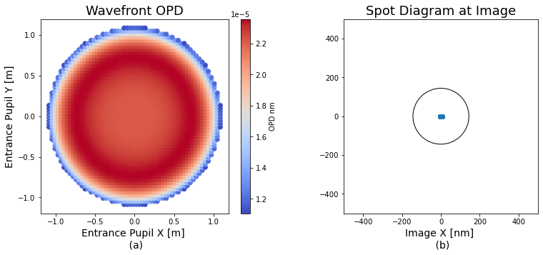
These data can be accessed directly from the Rayfront object. They are numpy arrays whose axes correspond to rayset, surface, and then ray (see the example in Listing 4). With the basic attributes, we can perform simple analyses such as spot diagrams or examining the OPD of the ray bundle at the exit pupil (shown in Figure 2.
We can access the coordinates at any surface in the optical system, which means that the totality of ray-based analyses can be built in Poke. However, Poke’s primary utility is to serve as a platform for ray-based physical optics. In the next section we illustrate two key physics modules built into Poke that can simulate diffraction and polarization from purely ray data.
3 Physical Optics Modules
Poke was developed with the intention of adding more open-source propagation physics to existing diffraction modeling packages. The two primary physics packages that use ray data are Gaussian Beamlet Decomposition and Polarization Ray Tracing.
3.1 Gaussian Beamlet Decomposition
Traditionally, physical optics propagators employ diffraction integrals derived from the Huygens-Fresnel principle. Plane-to-plane propagation is done with the Fresnel diffraction integral typically by using the angular spectrum method to model the transfer function of free space using a Fast Fourier Transformation. However, using these diffraction integrals imposes the scalar and paraxial assumption on the optical system of interest. This limits the scope of what the diffraction model can accurately determine.
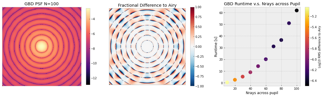
Gaussian Beamlet Decomposition (GBD) is an alternative method of physical optics propagation that has seen substantive implementation in commercial software. The operating principle of GBD is to decompose an arbitrary field into a finite sum of coherent Gaussian beamlets. The analytical propagation laws for these beamlets are known via ray transfer matrices, so they can be propagated along geometric ray paths. GBD doesn’t have an apparent presence in the open source. This is likely because a clear algorithm for its implementation is not present in the literature. We derived a method for its implementation and built it into Poke to study its suitability for high-contrast imaging[6]. The operating principle of GBD is exhaustively covered in the literature [7, 8, 9]. Because we know the analytic propagation laws of Gaussian beams, we can decompose an arbitrary wavefront into a finite sum of Gaussian beams and propagate them anywhere in a 3D non-paraxial optical system. In Figure 3 we show the ability of our poke.gbd module to reconstruct the analytical airy function. GBD requires that each beamlet is propagated to each point that we wish to know the field at. If we desire to propagate a field decomposed into to a plane that is in size, then the total number of propagations is equal to . This is a daunting challenge computationally, so careful consideration was built into the structure of our algorithm. All computation is vectorized, with the option to break it the simulation up into loops over the beamlet index should the simulation require more memory than a given computer has. We have also implemented accelerated computing options for computation on GPUs.
Optimizing the GBD technique is an active area of research for which Poke is a prime platform. It is ray tracer agnostic and can be studied by anyone with access to Python 3.8+. Furthermore, we believe this to be the first open-source implementation of the transfer-matrix method of GBD pioneered by Worku and Gross. Harvey et al [7] report on the complex ray tracing method implemented in FRED, which is the first known iteration of the technique. The transfer-matrix method generalizes the problem, enabling the propagation of any analytical solution to the general Collins’ integral[10, 6]. Consequently, we have the ability to alter the electric field profile of the Gaussian beamlets for higher-fidelity diffraction simulation.
3.2 Polarization Ray Tracing
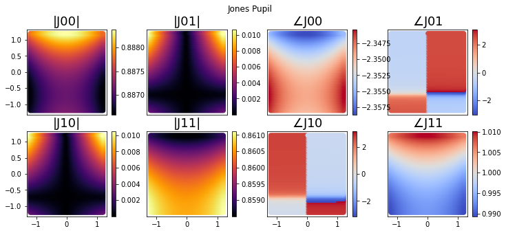
High-contrast imaging instruments in the next decade will be forced to contend with polarization aberrations[11]. The theory of polarization aberrations is described by McGuire and Chipman[12, 13], and Sasian[14]. These effects introduce low-order aberrations in even perfectly aligned optical systems, resulting from the polarized interaction of light with material interfaces. Yun[15, 16] outlined the basics of Polarization Ray Tracing (PRT), an algorithm by which polarization aberrations can be diagnosed. An exhaustive review of the technique is covered in Yun and Chipman, and will not be explained in detail here, but we refer the readers to Polarized Light and Optical Systems[17] for a tutorial. PRT propagates the effects of Fresnel Reflections through a 3D optical system to understand the total vector field behavior. Most notably, PRT gives us access to the Jones pupil. This is a critical data product for conducting diffraction modeling with consideration for polarization aberrations. PRT has been implemented in commercial design codes (CODE V, Zemax), and POLARIS-M555https://airyoptics.com/polaris-m-software/, which operates in Mathematica. However, there isn’t an apparent package with support in the open source community. To address this need, we built PRT into Poke to bring the technique into Python 3.8+. Users can retain their optical system ray traces in their preferred software, but load the PRT data directly into a Python environment. Using Poke, one can generate a Jones pupil using the following code. In this example, we illustrate the polarization aberrations of a Cassegrain telescope with a fold mirror[18].
Poke can decompose the elements of the Jones pupil into Zernike polynomials to re-sample them onto a regularly spaced grid. We can then leverage poke.interfaces to export the data to a physical optics propagator to perform diffraction analysis.
Poke provides us with the platform we need to democratize PRT, while still being useful for investigators with access to commercial ray tracing licenses.
3.3 Homogeneous Thin Film Stacks
Corollary to PRT is the need to simulate thin film multilayer stacks. Polarization in optical systems is frequently caused by the thin films deposited on the optics. To accurately model these effects in PRT, we built poke.thinfilms to be able to encompass the influence of arbitrary stacks of homogeneous, linear, and isotropic thin films. We do so via the characteristic matrix[19], but shown below in Equations 1 and 2
| (1) |
| (2) |
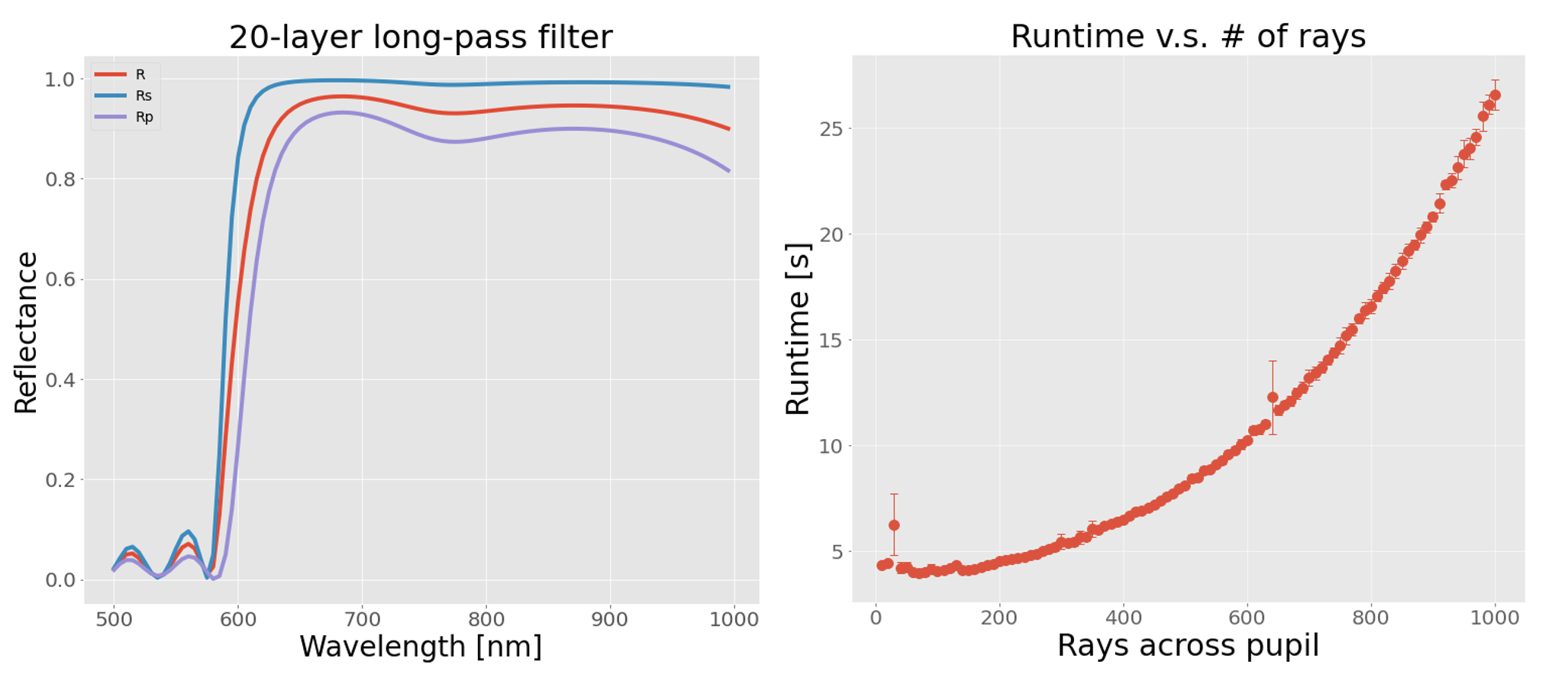
Equations 1 and 2 show the characteristic matrix from which the complex amplitude coefficients are readily derived. While this utility is useful in PRT simulations, it can be called independently to design thin film multilayer stacks. Below we show the design of a long pass filter using poke.thinfilms and scipy.minimize. This is an excellent example of the utility available to us by bringing these physical optics techniques into Python. In Figure 6 we illustrate a short-pass filter that was designed using the thin films module, and the runtime to compute a Jones pupil from this film data.
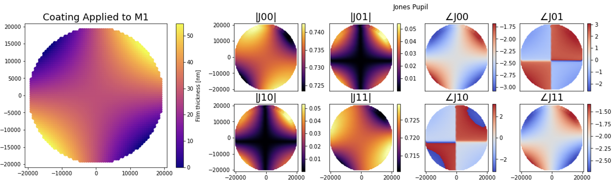
The thin film interface with optical surfaces is also compatible with spatially-varying thin films. This utility is critical in understanding how changes in film thickness can influence the Jones pupil of an optical system. In Figure 7 we apply an astigmatic coating to the primary mirror of the Extremely Large Telescope (ELT) and evaluate the Jones pupil. From these data, we are able to understand such a film’s influence on the amplitude and phase of our polarization state.
4 Integrated Modeling for Future Telescopes
Poke was inspired by the need to create a more integrated modeling pipeline for next-generation astronomical telescopes. Its capabilities to be an interface between commercial ray tracing codes and diffraction modeling software, while adding other ray-based utilities to the modeling pipeline, makes it a powerful design platform. Next-generation astronomical observatories include the 30m class ground-based Giant Segmented-Mirror Telescopes (GSMT’s) and the Astro2020-recommended Habitable Worlds Observatory (HWO).
4.1 Polarization Effect Modeling
Poke has already been used to model the nominal polarization aberrations present in the GSMT’s. In Anche et al [5] we discovered that the polarization aberrations due to the extremely large angles of incidence on the observatory mirrors lead to polarization aberration residuals that were greater than the desired contrast at the focal plane of ideal coronagraphic instrumentation. To achieve the baseline contrast proposed for these instruments, we must develop a method to mitigate the effect of polarization aberrations. In Ashcraft et al. in prep, we are developing an optimization-based method to design thin-film stacks to mitigate polarization aberrations.
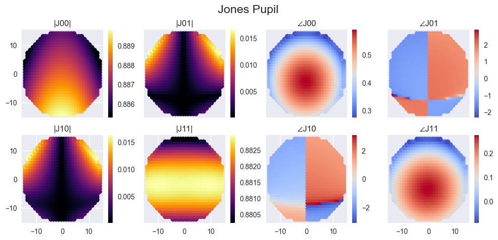
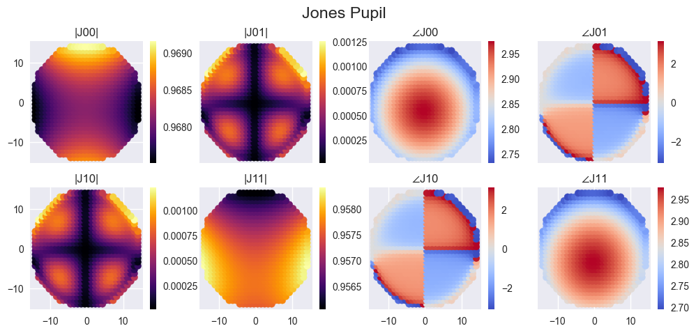
In Figures 8-9 we illustrate the results of using PRT with optimization routines in Python to design thin film stacks that can reduce the presence of polarization aberrations. This technique has potential implications for maximizing the achievable contrast near the inner working angle of coronagraphs for next-generation astronomical observatories.
4.2 High-performance Computing Options
Poke defaults to numpy for the vast majority of its numerical calculations. However, for high-fidelity simulations it is advantageous to employ Python packages with numpy-like API’s that grant the user more utility. Poke has adopted the interchangeable backend system of prysm (see section 4A of Dube et al[20]). Poke’s backend can be swapped from numpy to cupy for accelerated GPU-based computation, and jax to enable automatic differentiation.
cupy is an incredible Python package that allows users to scale their computations to GPUs without making significant changes to their code. It’s numpy-like API makes it trivial to implement in any codebase. GPUs are especially suited to large matrix multiplications, which are the fundamental operation of the physical optics modules discussed in Section 3.
jax is a Python package developed by Google that supports automatic differentiation (or autodiff). Autodiff enables the computation of analytic gradients without requiring the user to derive the analytic expression for gradient back-propagation. This is particularly useful for complex expressions, where the mathematics would grow unwieldy. jax makes Poke fully differentiable, enabling accurate computation of gradients for accelerated optimization.
5 Conclusions and Future Work
Poke is a new open-source ray-based physical optics engine written to further integrate the optical modeling pipeline. The availability of ray data in a Python environment democratizes the analysis done by ray tracing engines. The physics modules developed for Poke enhance the user’s simulation capabilities. This proceedings presents a brief overview of the utilities of Poke and their implications for modeling and design efforts in support of future astronomical observatories.
We are actively searching for collaborators to help build Poke. If you are interested in contributing, please contact the author or open an issue on our Github page666https://github.com/Jashcraf/poke[4] to start a discussion. Areas we are currently seeking to improve include:
-
1.
Interface with an open-source ray tracer
-
2.
Simulating the complex amplitude coefficients of liquid crystal thin films
-
3.
Simulating the complex amplitude coefficients of metasurfaces
-
4.
Exploring alternative beamlet profiles for more accurate beamlet decomposition techniques
-
5.
Contribution to examples in poke.readthedocs.io
-
6.
An active interface with commercial ray tracers for real-time interaction with optical system ray traces.
Acknowledgements.
Kian Milani and Kevin Derby contributed to the GPU compatibility. Brandon Dube wrote the function to read/write Rayfronts. Emory Jenkins wrote the Zernike polynomial generator. Ramya Anche and Trent Brendel contributed tests to the PRT and GBD modules, respectively. This work was funded by an NASA Space Technology Graduate Research Opportunity.References
- [1] Perrin, M., Long, J., Douglas, E., Sivaramakrishnan, A., Slocum, C., and others, “POPPY: Physical Optics Propagation in PYthon.” Astrophysics Source Code Library, record ascl:1602.018 (Feb. 2016).
- [2] Por, E. H., Haffert, S. Y., Radhakrishnan, V. M., Doelman, D. S., van Kooten, M., and Bos, S. P., “High Contrast Imaging for Python (HCIPy): an open-source adaptive optics and coronagraph simulator,” in [Adaptive Optics Systems VI ], Close, L. M., Schreiber, L., and Schmidt, D., eds., 10703, 1112 – 1125, International Society for Optics and Photonics, SPIE (2018).
- [3] Dube, B., “prysm: A python optics module,” Journal of Open Source Software 4(37), 1352 (2019).
- [4] Ashcraft, J. and hilltailor, “Jashcraf/poke: v1.0.1,” (May 2023).
- [5] Anche, R. M., Ashcraft, J. N., Haffert, S. Y., Millar-Blanchaer, M. A., Douglas, E. S., Snik, F., Williams, G., van Holstein, R. G., Doelman, D., Gorkom, K. V., and Skidmore, W., “Polarization aberrations in next-generation giant segmented mirror telescopes (GSMTs),” Astronomy and 672, A121 (apr 2023).
- [6] Ashcraft, J. N., Douglas, E. S., Kim, D., and Riggs, A., “Hybrid propagation physics for the design and modeling of astronomical observatories: A coronagraphic example,” SPIE Journal of Astronomical Telescopes, Instruments, and Systems (In Review).
- [7] Harvey, J. E., Irvin, R. G., and Pfisterer, R. N., “Modeling physical optics phenomena by complex ray tracing,” Optical Engineering 54(3), 1 – 12 (2015).
- [8] Worku, N. G. and Gross, H., “Propagation of truncated gaussian beams and their application in modeling sharp-edge diffraction,” J. Opt. Soc. Am. A 36, 859–868 (May 2019).
- [9] Greynolds, A. W., “Vector Formulation Of The Ray-Equivalent Method For General Gaussian Beam Propagation,” in [Current Developments in Optical Engineering and Diffraction Phenomena ], Fischer, R. E., Harvey, J. E., and Smith, W. J., eds., 0679, 129 – 133, International Society for Optics and Photonics, SPIE (1986).
- [10] Collins, S. A., “Lens-system diffraction integral written in terms of matrix optics,” J. Opt. Soc. Am. 60, 1168–1177 (Sep 1970).
- [11] Millar-Blanchaer, M. A., Anche, R. M., Nguyen, M. M., and Maire, J., “The polarization aberrations of the Gemini Telescope as seen by the Gemini Planet Imager,” in [Ground-based and Airborne Instrumentation for Astronomy IX ], Evans, C. J., Bryant, J. J., and Motohara, K., eds., 12184, 121843X, International Society for Optics and Photonics, SPIE (2022).
- [12] McGuire, J. P. and Chipman, R. A., “Polarization aberrations. 1. rotationally symmetric optical systems,” Appl. Opt. 33, 5080–5100 (Aug 1994).
- [13] McGuire, J. P. and Chipman, R. A., “Polarization aberrations. 2. tilted and decentered optical systems,” Appl. Opt. 33, 5101–5107 (Aug 1994).
- [14] Sasián, J., “Polarization fields and wavefronts of two sheets for understanding polarization aberrations in optical imaging systems,” Optical Engineering 53(3), 035102 (2014).
- [15] Yun, G., Crabtree, K., and Chipman, R. A., “Three-dimensional polarization ray-tracing calculus i: definition and diattenuation,” Appl. Opt. 50, 2855–2865 (Jun 2011).
- [16] Yun, G., McClain, S. C., and Chipman, R. A., “Three-dimensional polarization ray-tracing calculus ii: retardance,” Appl. Opt. 50, 2866–2874 (Jun 2011).
- [17] Chipman, R. A., Lam, W.-S. T., and Young, G., [Polarized light and optical systems ], CRC press (2018).
- [18] Breckinridge, J. B., Lam, W. S. T., and Chipman, R. A., “Polarization aberrations in astronomical telescopes: The point spread function,” Publications of the Astronomical Society of the Pacific 127(951), 445–468 (2015).
- [19] Peatross, J. and Ware, M., [Physics of Light and Optics ], optics.byu.edu (2015).
- [20] Dube, B. D., Riggs, A. J., Kern, B. D., Cady, E. J., Krist, J. E., Zhou, H., Nemati, B., Seo, B.-J., Steeves, J., Arndt, D., Mandić, M., Shields, J., Boussalis, D., Valverde, A., Rahman, Z., and Fathpour, N., “Exascale integrated modeling of low-order wavefront sensing and control for the Roman Coronagraph instrument,” Journal of the Optical Society of America A 39, C133 (Dec. 2022).