Poisson-Voronoi percolation in the hyperbolic plane
with small intensities
Abstract
We consider percolation on the Voronoi tessellation generated by a homogeneous Poisson point process on the hyperbolic plane. We show that the critical probability for the existence of an infinite cluster is asymptotically equal to as This answers a question of Benjamini and Schramm [9].
1 Introduction and statement of main result
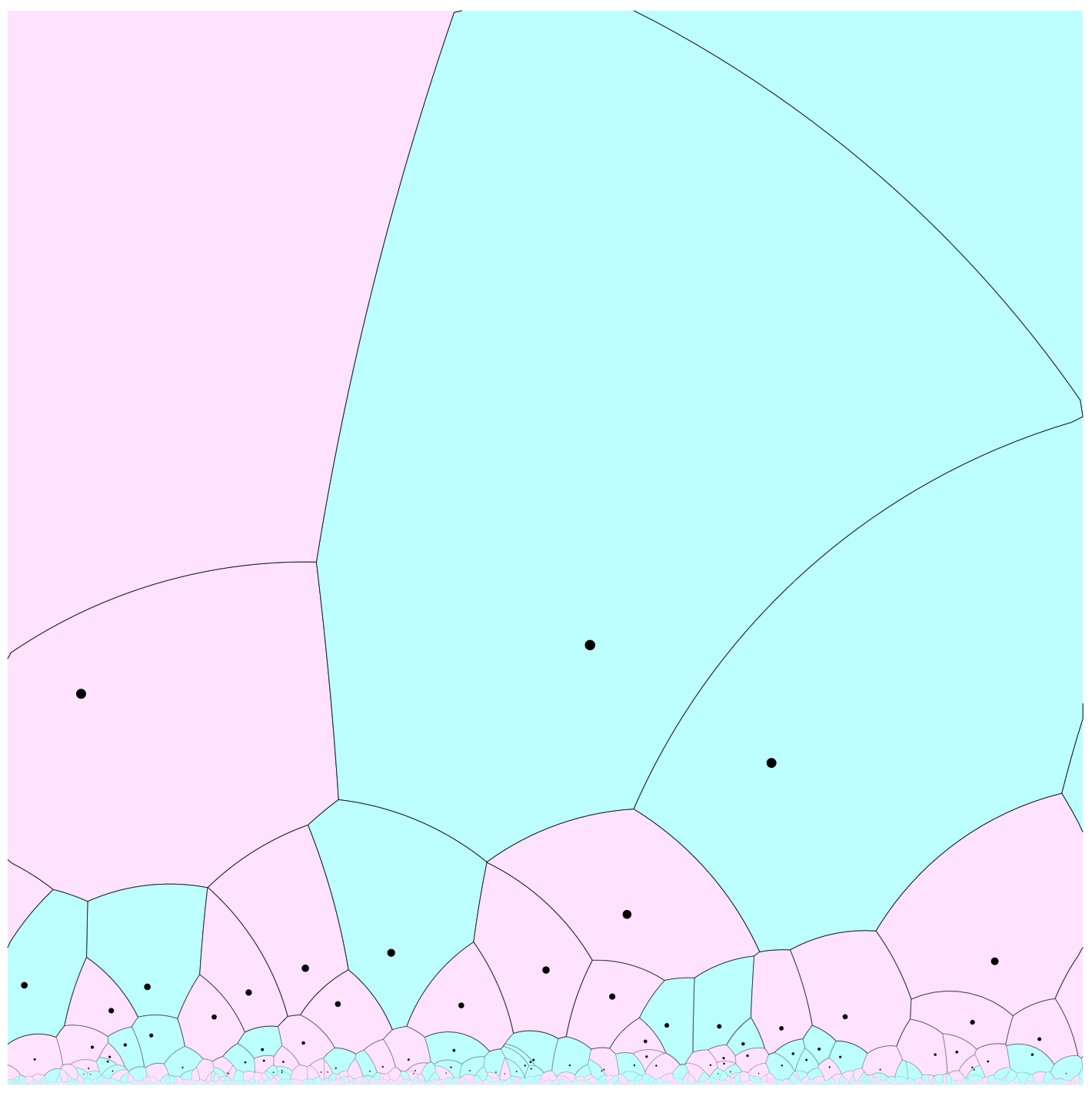
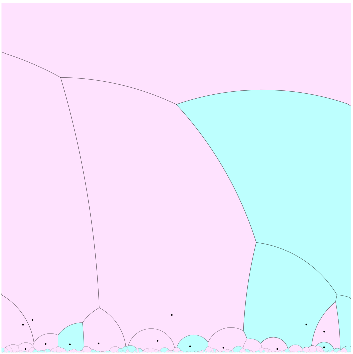
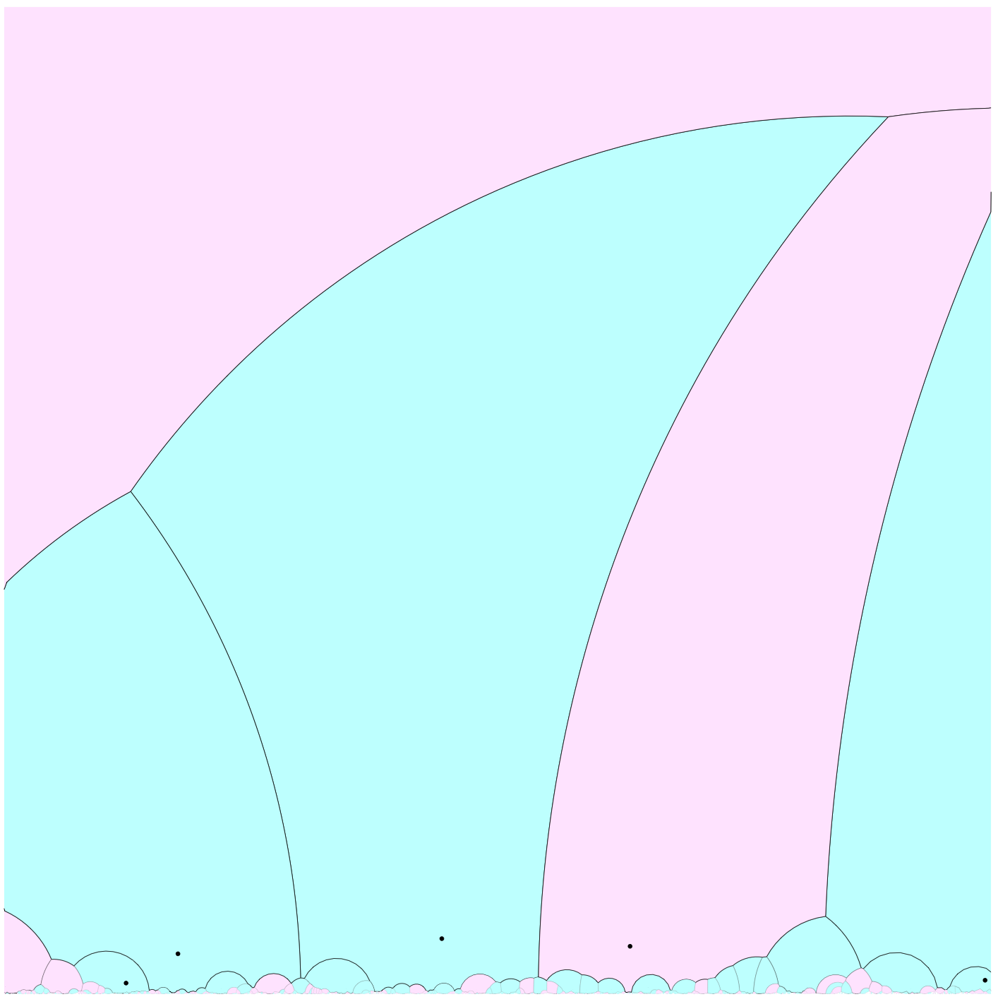
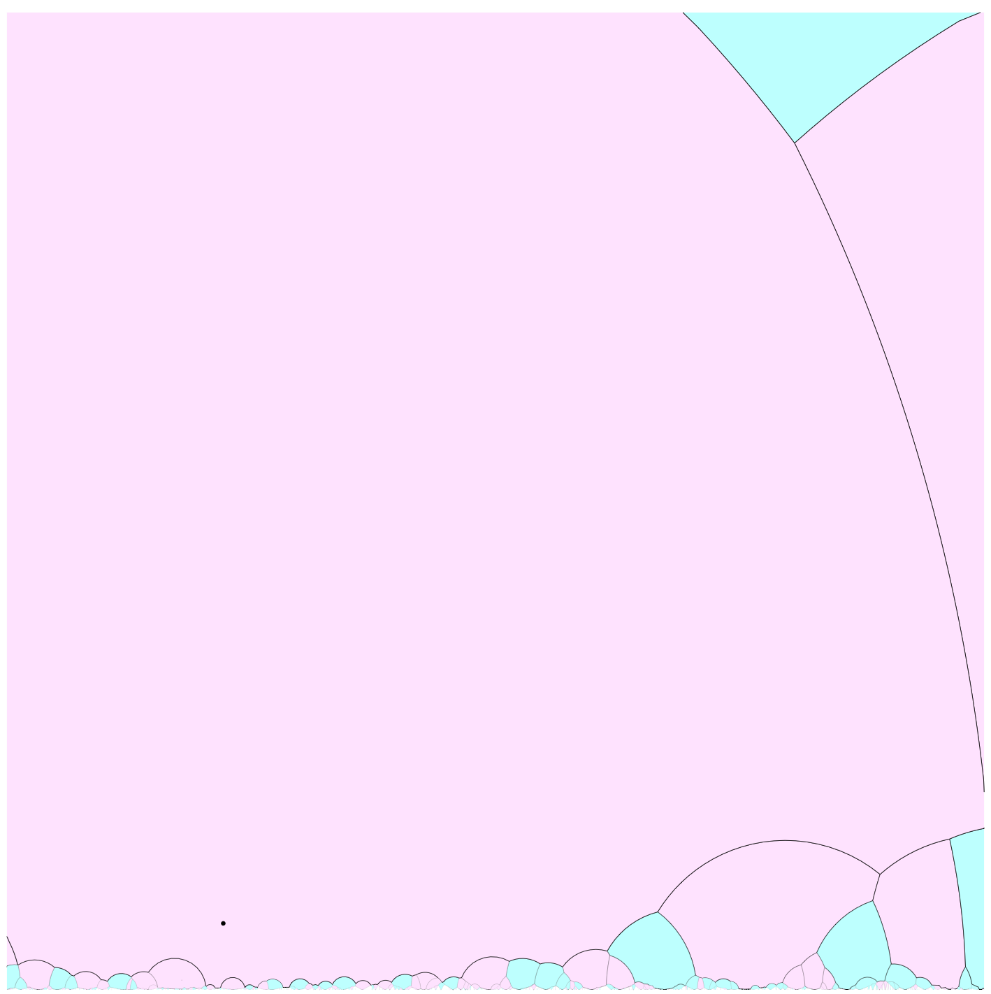
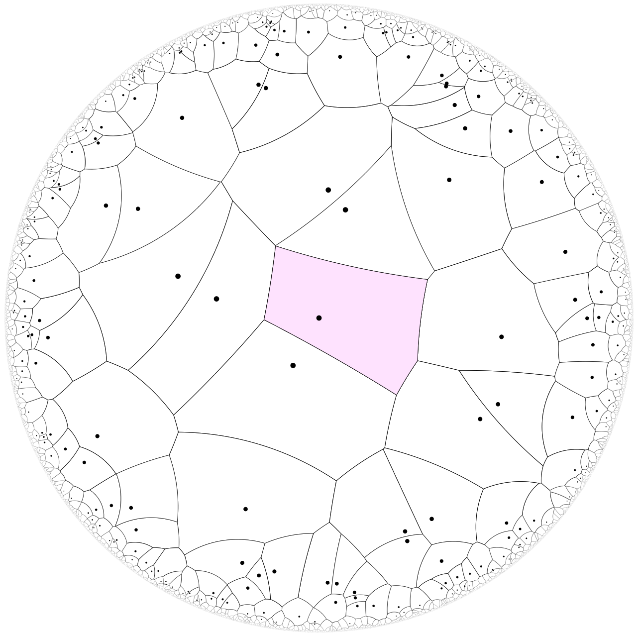
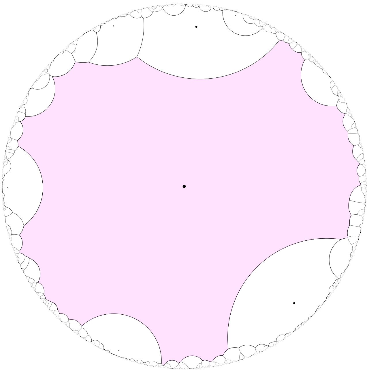
We will study percolation on the Voronoi tessellation generated by a homogeneous Poisson point process on the hyperbolic plane . That is, with each point of a constant intensity Poisson process on we associate its Voronoi cell – which is the set of all points of the hyperbolic plane that are closer to it than to any other point of the Poisson process – and we colour each cell black with probability and white with probability , independently of the colours of all other cells. See Figure 1 for a depiction of computer simulations of this process.
We say that percolation occurs if there is an infinite connected cluster of black cells. For each intensity of the underlying Poisson process, the critical probability is defined as
To the best of our knowledge, hyperbolic Poisson-Voronoi percolation was first studied by Benjamini and Schramm in the influential paper [9]. Amongst other things, they showed that for all ; that is a continuous function of ; and that as .
They also asked for the asymptotics of as , and specifically for “the derivative at ”. Here we answer this question, by showing:
Theorem 1
as
For comparison, Benjamini and Schramm gave an upper bound , whose asymptotics are as .
The results of Benjamini and Schramm highlight striking differences between Poisson-Voronoi percolation in the hyperbolic plane and Poisson-Voronoi percolation in the ordinary, Euclidean plane. For starters, in the latter case it is known [50, 10] that the critical probability equals for all values of the intensity parameter . More strikingly perhaps is the difference in the behaviour of the number of infinite, black clusters. In the Euclidean case there are no infinite black clusters when and precisely one infinite black cluster otherwise (almost surely). For the hyperbolic case, Benjamini and Schramm showed that if all black clusters are finite; if then there is precisely one infinite black cluster; but if then there are infinitely many, distinct, infinite, black clusters (almost surely).
Related work. Percolation theory is an active area of modern probability theory with a considerable history, going back to the work of Broadbent and Hammersley [12] in the late fifties. By now there is an immense amount of research articles, mostly centered on percolation on lattices. We direct the reader to the monographs [11, 22] for an overview.
Poisson-Voronoi tessellations (mostly in -dimensional, Euclidean space) are one of the central models studied in stochastic geometry. They are studied in connection with many different applications and have a long history going back at least to the work of Meijering [34] in the early fifties. For an overview, see the monographs [37, 39] and the references therein.
In the early nineties, Vahidi-Asl and Wierman [46] introduced first passage percolation (a notion related to, but distinct from percolation as we have defined it above) on planar, Euclidean Poisson-Voronoi tessellations. A few years later, Zvavitch [50] proved that in the Euclidean plane almost surely all black clusters are finite when (and arbitrary). About a decade after that Bollobás and Riordan were able to complement this result by showing that, almost surely, there exists an infinite black cluster when (and arbitrary) – thus establishing for planar, Euclidean Poisson-Voronoi percolation. Since then planar, Euclidean Poisson-Voronoi percolation, especially “at criticality”, has received a fair amount of additional attention. See e.g. [1, 2, 41, 49]. Poisson-Voronoi percolation on the projective plane was studied by Freedman [17], and Poisson-Voronoi percolation on more general two and three dimensional manifolds was studied by Benjamini and Schramm in [8]. Poisson-Voronoi percolation on higher dimensional Euclidean space has been studied as well, in [4, 3, 15].
Fuchsian groups can be seen as the analogue in the hyperbolic plane of lattices in the Euclidean plane. Lalley [29, 30] studied percolation on Fuchsian groups and amongst other things established that the critical probabilities for “existence” and “uniqueness” of infinite clusters are distinct. Works on continuum percolation models over Poisson processes in the hyperbolic plane include [5, 16, 42, 44, 45]. Aspects of hyperbolic Poisson-Voronoi tessellations besides percolation that have been studied include the (expected) combinatorial structure of their cells, random walks on them and anchored expansions – see for example [6, 7, 13, 19, 26, 27]. Percolation on hyperbolic Poisson-Voronoi tessellations was first studied specifically by Benjamini and Schramm in [9]. In the recent paper [24] the current authors showed that as for Poisson-Voronoi percolation on the hyperbolic plane, proving a conjecture from [9].
Comparing Theorem 1 with Isokawa’s formula (stated as Theorem 6 below), we see that our result can be rephrased as : as , the critical probability is asymptotic to the reciprocal of the “typical degree” (defined precisely in Section 2.3 below). A similar phenomenon happens in several Euclidean percolation models when one sends the dimension to infinity. The most well-known result in this direction is probably that for both site and bond percolation on , we have that , as was shown concurrently and independently by Gordon [21], Hara and Slade [25] and Kesten [28]. Prior to that there were non-rigorous derivations of the result in the physics literature and Cox and Durret [14] had proved the analogous result for oriented percolation (which is technically easier to analyze). Penrose [36] proved an analogous result for the Gilbert model on -dimensional Euclidean space as the dimension tends to infinity, and Meester, Penrose and Sarkar [33] extended this result to the random connection model. The analogous phenomenon was shown by Penrose [35] for spread out percolation in fixed dimension when the connections get more and more spread out.
Sketch of the main ideas used in the proof. The intuition guiding the proof is that when is small and is of the same order as then black clusters are “locally tree like”, in the sense that while there will be some short cycles in the black subgraph of the Delaunay graph, but these will be “rare”. (The Delaunay graph is the abstract combinatorial graph whose vertices are the Poisson points and whose edges are precisely those pairs of points whose Voronoi cells meet.) This is also the intuition behind the results on high-dimensional and spread-out percolation mentioned above. In fact, in several of the works cited it is in fact shown that if we scale as a constant divided by the degree (so that the origin has black neighbours in expectation) then the cluster of the origin behaves more and more like a Galton-Watson tree with a Poisson offspring distribution as the dimension grows.
Before going further, it is instructive to informally discuss in a bit more detail the situation for the high-dimensional Gilbert model analyzed by Penrose in [36]. In that model, we build a random graph on a constant intensity Poisson process on by joining any pair of Poisson points at distance by an edge. We seek the critical intensity such that there is a.s. no percolation for and there is a positive probability of percolation when . We consider the scenario where is large and the intensity is with the volume of the -dimensional unit ball and a fixed constant. We add the origin to the Poisson process (note that this a.s. does not change whether or not there is an infinite component), and think of “exploring” the cluster of the origin. We do this in an iterative fashion : we first add the neighbours of the origin to the cluster, then we consider each of these neighbours in turn and add their neighbours to the cluster, and so on. Of course the neighbours of the origin are precisely those Poisson points that fall inside the -dimensional unit ball . In particular their number follows a Poisson distribution with mean . Once we have already added some points to the cluster of the origin and we consider the neighbours of a previously added point , we add those Poisson points that fall inside the ball of radius one around from which we have removed the union of all radius one balls around points we have processed already. Because of the high-dimensional geometry, the volume of this set difference is typically very close to the volume of a unit radius ball with nothing removed – at least during the initial stages of the exploration. In other words, at least during the first few exploration steps, the number of new points that gets added in each exploration step is approximately distributed like a Poisson random variable with mean . This naturally leads to the aforementioned connection with Galton-Watson trees with Poisson offspring distribution. Essentially, the geometric reason why this works out is the “concentration of measure” for high dimensional balls (see for instance [32], Chapter 13) : in high-dimensional Euclidean space, the volume of the unit ball is concentrated near its boundary. From this one can derive that, in a sense that can be made precise, most pairs of points connected by an edge in the Gilbert graph will have distance close to one. Moreover, the mass of a -dimensional ball is also concentrated near its equator, from which one can derive that – in a sense that can be made precise – for most pairs of points with a common neighbour, their distance will be very close to and, more generally, most pairs with graph distance will have Euclidean distance close to (for fixed).
A similar phenomenon, but maybe even more extreme in a sense, happens in the hyperbolic plane for disks of large radius : The area of a hyperbolic disk of large radius is concentrated near its boundary; and if we take two points at random from then typically their distance is close to , the maximal possible distance between any two points in . In the current paper, we consider a Poisson point process on the hyperbolic plane with small intensity . We again include the origin and try to analyze the black cluster of the Voronoi cell of the origin in the Voronoi tessellation for , where the cell of the origin is coloured black and all other cells are each coloured black with probability and white with probability . By Isokawa’s formula (stated as Theorem 6 below) the expected number of cells that are adjacent to the cell of the origin is asymptotic to as tends to zero. Moreover, as can be seen either by looking more carefully at Isokawa’s computations or by reading some of our arguments below, it can be shown that most neighbours of the origin are at distance close to . Note that goes to infinity as . Now suppose we take with a constant and small, so that the expected number of black cells neighbouring the cell of the origin is close to . If we follow an exploration process analogous to the one described above for the Euclidean Gilbert model, the black cluster will have the property that most pairs of points at graph distance have distance close to in the hyperbolic metric.
For the upper bound, we will show that if and is sufficiently small (and is a fixed constant) then the size of the black cluster of the origin stochastically dominates the size of a supercritical Galton-Watson tree. We will use an exploration procedure similar to what we described above for the high-dimensional Gilbert model. During the exploration, when we consider some point that has already been added to the tree, we make sure to only add those black neighbours of whose distance to is within some large constant of . We also make sure to select a subset of these neighbours with the property that all angles are larger than some small constant, and moreover for each there is a ball of radius some large (but fixed) constant that contains no other Poisson points. Essentially because of the geometric phenomena described earlier, it will turn out that in this version of the exploration procedure, for sufficiently small , the subgraph of the cluster of the origin we obtain follows the distribution of a certain supercritical Galton-Watson process exactly. In contrast, in the high-dimensional Gilbert model the correspondence between the exploration process and a supercritical Galton-Watson process will eventually break down, after a (large) number of exploration steps that depends on the dimension, so that additional techniques and arguments were needed by Penrose [36].
For hyperbolic Poisson-Voronoi percolation the lower bound is technically more involved than the upper bound. This is probably the most novel contribution in our paper, and we believe it might inspire similar arguments applicable to other problems in percolation, notably for high-dimensional models. For percolation on and the Gilbert model, a trivial (and “sharp” up to lower order corrections when ) lower bound is given by a comparison to branching processes : in the former model, the cluster of the origin is stochastically dominated by a Galton-Watson distribution with mean offspring and in the latter with mean offspring . So the critical probability satisfies , respectively the critical intensity satisfies . (For percolation on this was in fact already observed by Broadbent and Hammersley [12] and for the Gilbert model by Gilbert [18].) In our case a similar argument does not seem feasible. In the Gilbert model, imagine we have explored part of the cluster of the origin and in doing so have revealed the status of the Poisson process in some region. We now wish to add those neighbours that are not yet part of the cluster of a point that we have previously added to in the cluster. The number of new points added is stochastically dominated by the number of new points we add at the very start of the exploration, when add the neighbours of the origin. In the Poisson-Voronoi percolation model there is no obvious monotonicity of this kind. Once we have revealed the status of the Poisson point process in some region this can make new edges both more and less likely. As a side remark, let us mention that using the methods in our paper it ought to be possible to show that when then, as , the size of black cluster of the origin will converge in distribution to the size of a Galton-Watson tree with Poisson offspring distribution. We do not pursue this here however as it does not appear useful for bounding : it will not exclude the possibility that – for any fixed, small – there is an extremely small, but positive probability that the origin is in an infinite component.
A naive approach that one might try is to compute the expected number of black paths of length starting at the origin (for small and ), and hope to show that this expectation tends to zero as . Unfortunately this approach does not seem feasible either. Long paths might revisit the same area many times which introduces dependencies that are difficult to deal with.
In order to circumvent this issue, we introduce what we call linked sequences of chunks. As we wish to show percolation does not occur, it suffices to show no infinite black cluster exists with a more generous notion of adjacency, in the form of what we call pseudo-edges, that makes the analysis simpler. With each pseudo-edge we associate a “certificate”, being the region of the hyperbolic plane that needs to be examined to verify it is indeed a pseudo-edge. We’ll say a pseudo-edge on a path is good if it has length close to and does not make a small angle with the previous pseudo-edge. Otherwise it is bad. A linked sequence of chunks is a sequence of paths such that: 1) on each path, every pseudo-edge except the last is good and the last is bad, and 2) for each , either the first point of is close to the certificate of some pseudo-edge of or the certificate of the first pseudo-edge of intersects one of the certificates of , and for every other pseudo-edge of its certificate is disjoint from all certificates of all pseudo-edges on . We’ll first show (Proposition 31 below) that if the cluster of the origin is infinite, then either there exists an infinite path all of whose edges are good, or there exists an infinite linked sequence of chunks starting from the origin. Unlike paths in general, it is technically feasible to give decent bounds on the expected number of good paths, respectively the number of linked sequences of chunks, of some given length . We are able to obtain bounds that tend to zero with , which implies no percolation occurs a.s.
Structure of the paper. In the next section, we collect some notations, definitions, facts and tools that we will need in our proofs. Section 3.1 contains some preparatory geometric observations needed in later sections. Section 3.2 contains the proof that for small enough (and fixed), and Section 3.3 contains the proof that for small enough . We end the paper by suggesting some directions for further work in Section 4.
2 Notation and preliminaries
2.1 Ingredients from hyperbolic geometry
The hyperbolic plane is a two dimensional surface with constant Gaussian curvature . There are many models, i.e. coordinate charts, for including the Poincaré disk model, the Poincaré half-plane model, and the Klein disk model. A gentle introduction to Gaussian curvature, hyperbolic geometry and these representations of the hyperbolic plane can be found in [38].
Even though we used the Poincaré half-plane model for the visualizations in Figure 1, from now on we will exclusively use the Poincaré disk model. (A computer simulation of Poisson-Voronoi percolation depicted in the Poincaré disk model can be found on the second page of our earlier paper [24].) We briefly recollect its definition and some of the main facts we shall be using in our arguments below, and refer the reader to [38] for proofs and more information.
The Poincaré disk model is constructed by equipping the open unit disk with an appropriate metric and area functional. For points the hyperbolic distance can be given explicitly by
where denotes the Euclidean norm. Straightforward calculations show that in particular, for , the Euclidean and hyperbolic distance to the origin are related via:
| (1) |
We will use the notations
for hyperbolic, respectively Euclidean, disks. A standard fact that we will rely on in the sequel is:
Fact 2
Every hyperbolic disk is also a Euclidean disk; and every Euclidean disk contained in the open unit disk is also a hyperbolic disk.
(But, the centre and radius of a disk with respect to the hyperbolic metric do not coincide with the centre and radius with respect to the Euclidean metric.)
For any measurable subset its hyperbolic area is given by
where
| (2) |
From the formulas for hyperbolic distance and hyperbolic area one can derive that:
| (3) |
The hyperbolic polar coordinates corresponding to a point are and is the (counterclockwise) angle between the positive -axis and the line segment . Put differently, and and are such that
| (4) |
In several computations in the paper we’ll use the change of variables to hyperbolic polar coordinates. By this we of course just mean applying the substitution (4). We will always apply it to integrals of the form with as given by (2) above, to obtain:
| (5) |
A hyperbolic geodesic or hyperbolic line segment between two points is the shortest path between and with respect to the hyperbolic metric. If there is a (Euclidean) line passing through and the origin , then the hyperbolic geodesic between and is just the (ordinary) line segment between them. Otherwise, the hyperbolic geodesic between can be constructed geometrically as follows. We let be the unique (Euclidean) circle with and such that it hits the boundary of the unit disk at right angles. The points divide into two circle segments. The hyperbolic geodesic between and is the one contained in .
A hyperbolic line is either the intersection of an Euclidean line through the origin with the open unit disk , or the intersection of with a circle hitting at right angles.
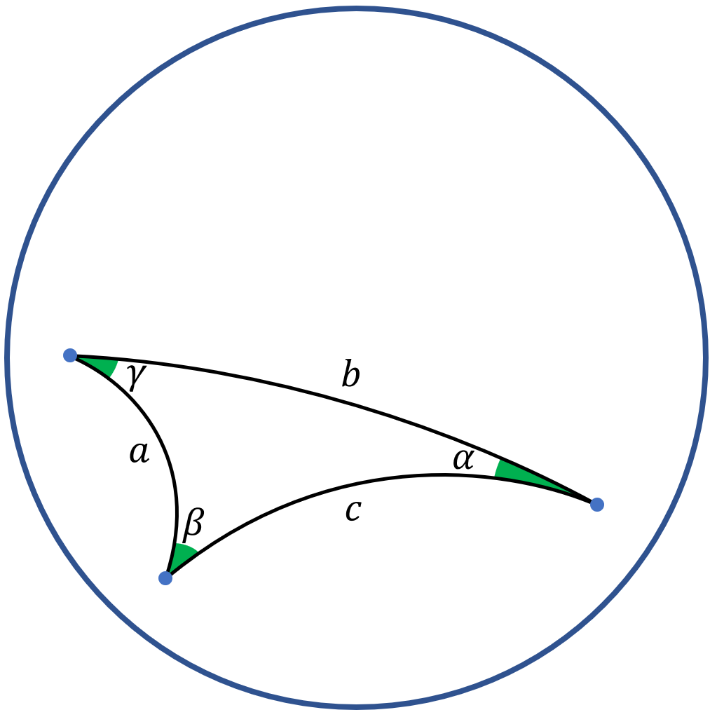
If then we use to denote the angle the hyperbolic line segment between and and the hyperbolic line segment between and make in the common point . (In general, when do not lie on a hyperbolic line, there will be two possible interpretations of this angle, one in and one in . As is usual, we shall always take the smaller of the two.) A hyperbolic triangle is the set of the three hyperbolic line segments defined by three (non-collinear) points . A critical tool is hyperbolic law of cosines. A proof of this result can for instance be found in [43] (page 81).
Lemma 3
For a hyperbolic triangle, with sides of length and respective opposite angles (see Figure 2):
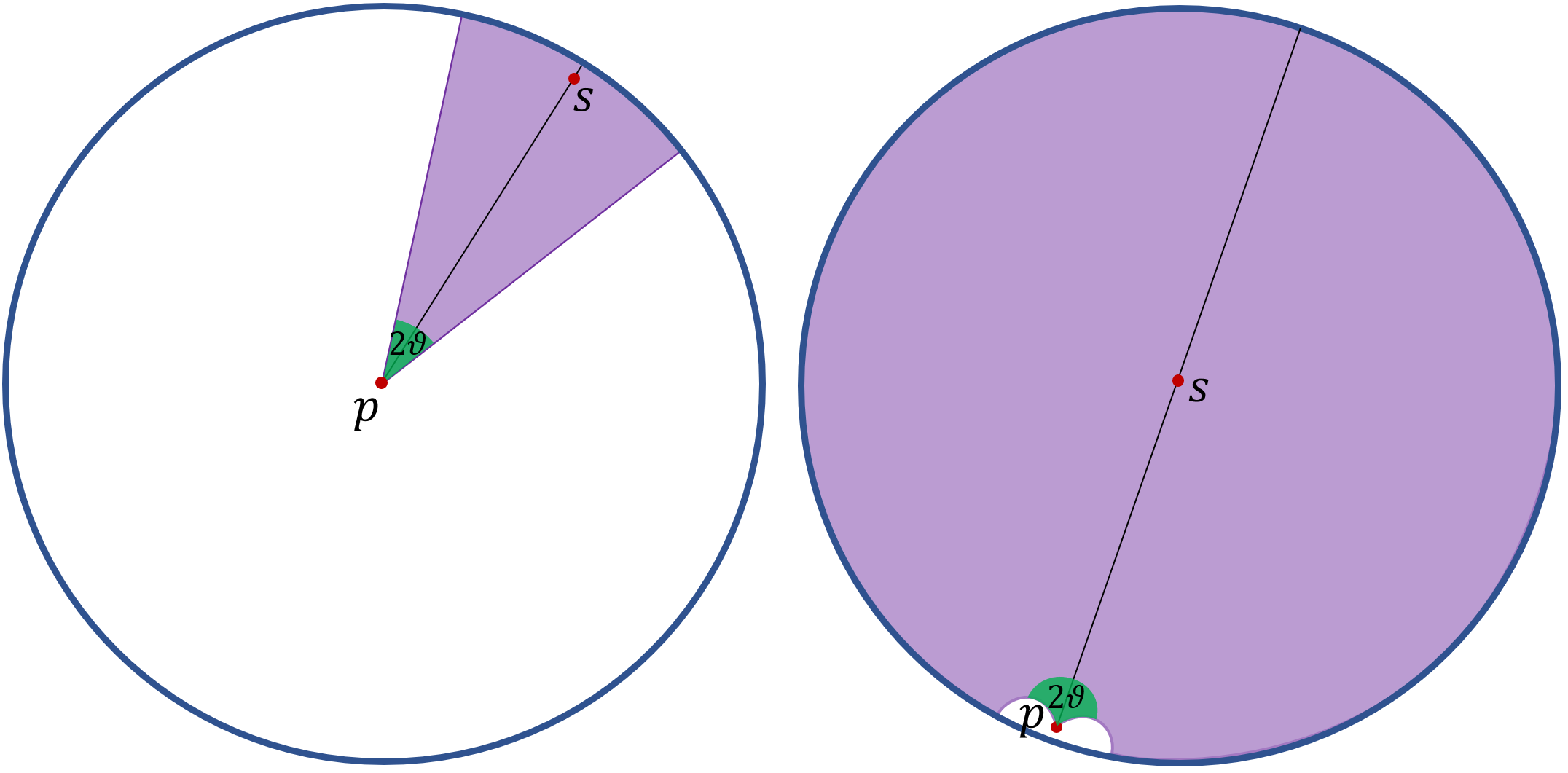
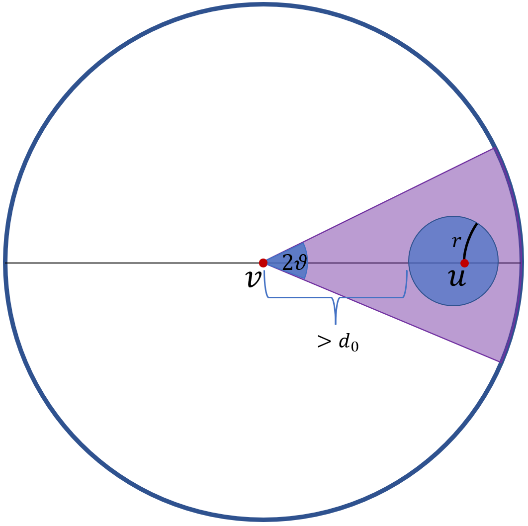
A hyperbolic ray is defined analogously to a ray in Euclidean geometry. That is, if is a hyperbolic line then any divides into two connected components. Each of these is a ray emanating from . For distinct and we let denote the set of all hyperbolic rays emanating from that make an angle of no more than with the ray emanating from through . In particular, in the Poincaré disk model, if is the origin then looks like a (Euclidean) disk sector of opening angle with bisector the ray emanating from through . See Figure 3. For any other , the set can be obtained by applying a suitable hyperbolic isometry to such a disk sector.
A hyperbolic isometry is a bijection that preserves hyperbolic distance, i.e. for all . For any two points in , there exists a unique hyperbolic line through and , and there exists a hyperbolic isometry such that is an open interval given by the line segment between and , is the origin and is on the positive x-axis. In addition to distance, hyperbolic isometries preserve angles, in the sense that if are curves (e.g. hyperbolic line segments, circles, …) that meet in the point at angle , then the curves meet in the point at the same angle . Hyperbolic isometries also preserve hyperbolic area. That is,
| (6) |
for all (measurable) and every hyperbolic isometry . What is more, if is a hyperbolic isometry then, for any (integrable) we have
| (7) |
with as defined by (2). (An easy way to see this is to first note it follows trivially from (6) when is the indicator function of some measurable . From this it easily follows for step-functions . Then it follows for an arbitrary measurable function, by approximating it arbitrarily closely by step functions.)
2.2 Hyperbolic Poisson point processes
In the rest of this paper will denote a homogeneous Poisson point process (PPP) on the hyperbolic plane. Analogously to homogeneous Poisson point processes on the ordinary, Euclidean plane, a homogeneous Poisson process of intensity on the hyperbolic plane is characterized completely by the properties that a) for each (measurable) set the random variable is Poisson distributed with mean , and b) if are (measurable and) disjoint then the random variables are independent. In the light of the formula for above, we can alternatively view as an inhomogeneous Poisson point process on the ordinary, Euclidean plane with intensity function
with given by (2) above.
Throughout the remainder, we attach to each point of a randomly and independently chosen colour. (Black with probability and white with probability .) We let denote the black points and the white points of . In the language of for instance [31], we can view as a marked Poisson point process, the marks corresponding to the colours.
We will rely heavily on a specific case of the Slivniak-Mecke formula, which is our weapon of choice for counting tuples of points satisfying a given property. Before stating it, we remind the reader that formally speaking a Poisson process on is a random variable that takes values in the space of locally finite subsets of , equipped with the sigma algebra generated by the family events of the form : a given Borel set contains precisely points.
Theorem 4 (Slivniak-Mecke formula)
Let be a homogeneous hyperbolic Poisson point process of intensity , and let Let be a nonnegative, measurable function. Then
with given by (2).
As mentioned above, the version we state here is a specific case of a more general result. The general version can for instance be found in [37], as Corollary 3.2.3. (The version we present here is the special case of Corollary 3.2.3 in [37] when the ambient space and the intensity measure has density with as in (2).) The Slivniak-Mecke formula is sometimes also called Mecke formula or Campbell-Mecke formula in the literature.
We shall be applying the following consequence of the Slivniak-Mecke formula, that is tailored to our situation where and membership in is determined via independent, -biased coin flips.
Corollary 5
For and , let be as above and let be a nonnegative, measurable function. Then
with given by (2).
Proof. Let us write
We imagine first “revealing” the locations of the Poisson points , but not yet the colours/coin flips. For any fixed, locally finite we have
while
This holds for every locally finite , which implies
The result now follows by applying the Slivniak-Mecke formula to .
2.3 Hyperbolic Poisson-Voronoi tessellations
For a countable point set and we will denote the corresponding hyperbolic Voronoi cell of by:
We will usually suppress the second argument, and just write for the Voronoi cell of ; and will usually be either a homogeneous hyperbolic Poisson process or , such a Poisson process with the origin added in.
The hyperbolic Delaunay graph for is the abstract combinatorial graph with vertex set and an edge if the Voronoi cells meet. So we can alternatively view hyperbolic Poisson-Voronoi percolation as site-percolation on the hyperbolic Poisson-Delaunay graph. We say that are adjacent if they share an edge in the Poisson-Delaunay graph (in other words, the Voronoi cells have at least one point in common). In this case we will also say that are neighbours.
We point out that if then it must hold that and . In other words are adjacent if and only if there is hyperbolic disk such that and . Although we shall not be using this in the present paper, it may be instructive to the reader to point out the following. By this last observation, Fact 2 and some relatively straightforward probabilistic considerations : if is a homogeneous, hyperbolic Poisson process then, almost surely, the Voronoi tessellations for with respect to the ordinary, Euclidean metric and the Voronoi tessellation with respect to the hyperbolic metric as defined above have the same combinatorial structure, in the sense that are adjacent in the Euclidean tessellation if and only if they are adjacent in the hyperbolic tessellation. See Lemma 5 in our previous paper [24].
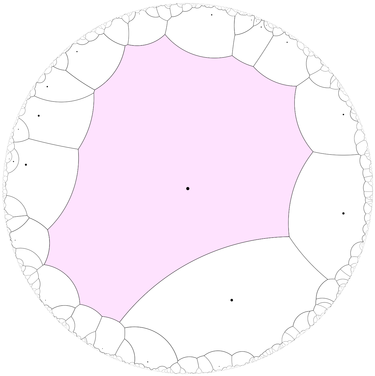
In many of our arguments below we will be considering the Voronoi tessellation for , a homogeneous, hyperbolic Poisson process with the origin added in. We refer to the origin as the typical point and to its Voronoi cell as the typical cell. See Figure 4 for computer simulations of the typical cell, shown in the Poincaré disk model, for various choices of .
We define the typical degree as
| (8) |
The typical degree for homogeneous, hyperbolic Poisson processes has previously been studied by Isokawa [27]. She gave the following exact formula for its expectation, valid for all values of the intensity parameter .
What is important for us is the asymptotics as . An independent, alternative derivation of these asymptotics, using conceptually simple arguments that are similar to the ones we will use in the present paper, is given in Chapter 3 of the doctoral thesis of the first author [23].
It may be instructive for the reader (but does not enter into the arguments in the present paper) to point out that as the expected typical degree tends to 6, the value for the expected typical degree in planar, Euclidean Poisson-Voronoi tessellations [34].
3 Proofs
3.1 Drawing trees in the hyperbolic plane
We will find it useful to consider graphs embedded in the hyperbolic plane. From now on every graph in the rest of the paper, has vertices that are points in the Poincaré disk, and we identify each edge with the (hyperbolic) geodesic line segment between and .
Definition 7
For we say that is a -tree if it is connected and
-
(i)
For every edge we have ;
-
(ii)
If the edges have a common endpoint , then the angle they make at is at least .
We will speak of a -path if the -tree is a path.
The following proposition verifies that we are justified in using the word “tree” : a -tree is also a tree in the graph theoretical sense, at least when the parameter is sufficiently large.
Proposition 8
For every there exists such that, for all , every -tree is acyclic.
We have to postpone the proof until some necessary preparations are out of the way. If is a -tree then clearly the hyperbolic distance between any two vertices is upper bounded by . Here and in the rest of the paper, denotes the graph distance, i.e. the number of edges on the (unique) -path in .
The following proposition shows that for sufficiently large this trivial upper bound is close to being tight.
Proposition 9
For every there exists and such that, for all , every -tree and for every two vertices :
Again we postpone the proof until we have made some additional observations.
If is a graph and then we denote by the connected component of that contains . In other words, is the subgraph induced on all nodes other than that can be reached from using a path that avoids .
The following observation is an important ingredient in the proof of our main result.
Proposition 10
For all there exist and such that, for all every -tree and every edge :
Again we have to postpone the proof until we have made some more preparatory observations. The next few Lemma’s in this section are technical (hyperbolic) geometric considerations that are intermediate steps in the proof of the three propositions above. When reading the paper for the first time, the reader may wish to only read the lemma statements and skip over the proofs.
We start with a relatively straightforward, but for us useful, consequence of the hyperbolic cosine rule.
Lemma 11
For every there exists such that the following holds for every hyperbolic triangle. Let the lengths of the sides be and and the respective opposing angles as in Figure 2. If then
Proof. We can assume without loss of generality that . For any hyperbolic triangle satisfying the hypothesis of the lemma, we have
The second line is the hyperbolic law of cosines (Lemma 3). The third line follows as and is decreasing on . The fourth line uses that and and (by assumption). Taking logs, we find
Next, we show that if are at least apart with a (large) constant and arbitrary then, from the point of view of (i.e. if we isometrically map to the origin of the Poincaré disk), a ball of large constant radius around will be contained in a sector of small opening angle.
Proof. We let be a large constant, to be determined in the course of the proof. Applying a suitable isometry if needed, we can assume without loss of generality that is the origin and lies on the positive -axis. We recall that is also a Euclidean disk. Its Euclidean center must lie on the -axis. (This is for instance easily seen by noting that the reflection in the -axis is a hyperbolic isometry that fixes , and hence leaves invariant.)
By the triangle inequality and the assumption that , we have
By (1), for each we have
where is a small constant to be determined shortly, and the final inequality holds provided we have chosen sufficiently large. Since is contained in the annulus , its Euclidean radius is no more than .
As its Euclidean centre lies on the -axis, it is clear that can be chosen so that .
Our next observation is another intermediate step in the proofs of Propositions 8, 9 and 10. It will be used only in the proof of Lemma 14 that immediately succeeds it in the text.
Lemma 13
Suppose the (Euclidean) circle intersects the unit circle at right angles, and intersects the -axis at an angle . If denotes the (Euclidean) radius of and denotes the intersection point of and the -axis that falls inside , then
Proof. Let denote the centre of . Since hits the unit circle at a right angle, we have . In the Euclidean triangle with corners , the angle at equals . See Figure 6.
Applying the Euclidean cosine rule to the triangle with corners we find
The claimed expression follows by reorganizing this last identity.
The next lemma makes the following perhaps rather counterintuitive observation. While looks “large” from the vantage point of (i.e. if we isometrically map to the origin of the Poincaré disk, the sector looks only like a small “slice”), provided are sufficiently far apart, from the vantage point of the set is actually contained in a small “slice”.
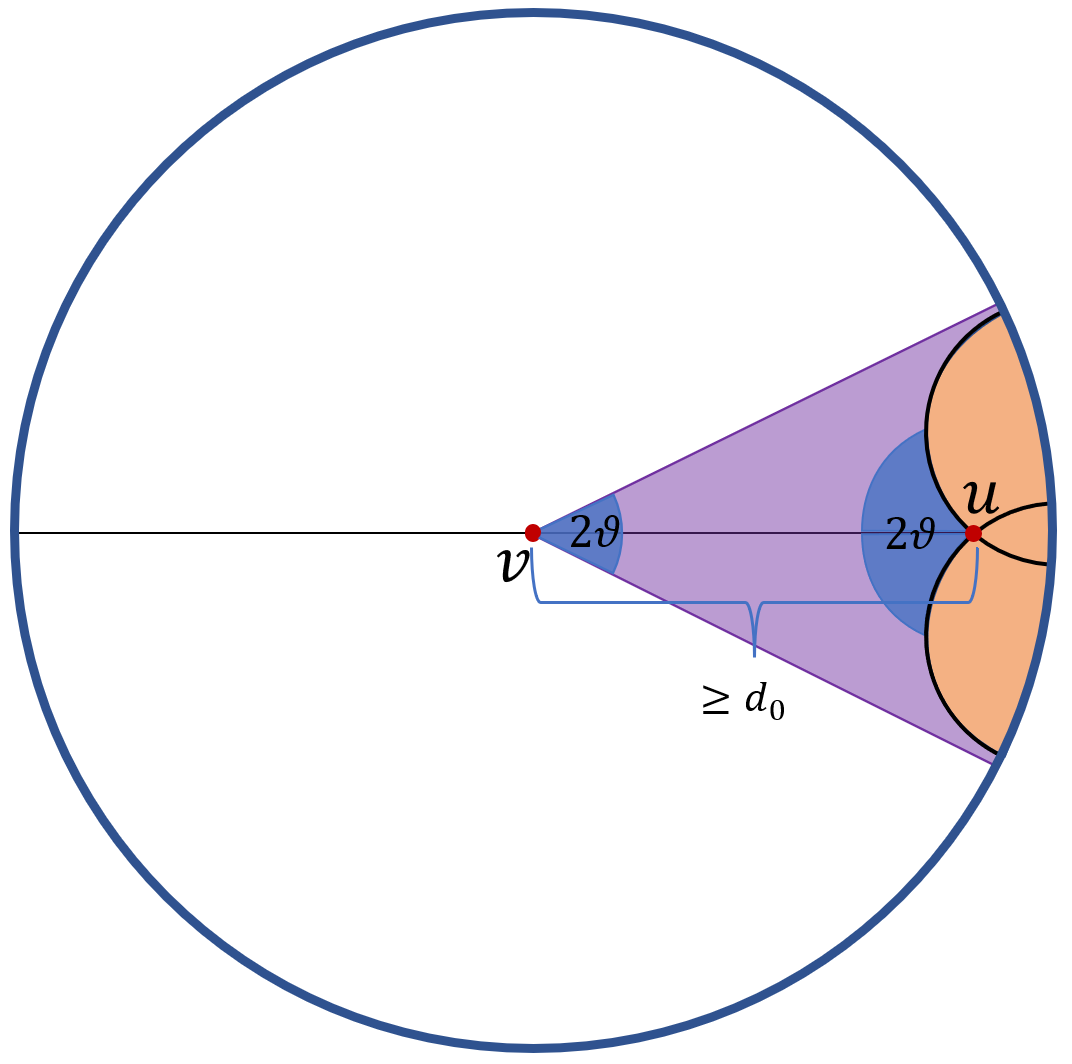
Proof. Applying a suitable isometry if needed, we can assume without loss of generality that is the origin and lies on the positive -axis.
The boundary of consists of two rays emanating from that each make an angle with the hyperbolic line through and at (and a circle segment that is part of the unit circle ). In Euclidean terms, these two rays are circle segments of circles that each meet the -axis in at an angle of , and intersect the boundary of the unit circle at right angles. (See Figure 7.) Let us call these circles . Both circles meet the -axis in at angle . Hence, by Lemma 13, both have Euclidean radius .
We have which approaches one as approaches infinity. In particular, for any constant , we can choose the constant so that both have Euclidean radius , and both intersect the -axis at a point within distance of . In other words, we’ll have
Clearly, if we take small enough, it now follows that , as desired.
As our final preparation for the proofs of Propositions 8 and 9, we show that if is a -tree and an edge then the vertices of are all contained in a small sector from the vantage point of , provided is chosen sufficiently large.
Lemma 15
For every there exists a such that, for every , every -tree and every edge :
Proof. We can and do assume, without loss of generality, that and ; and we set with as provided by Lemma 14.
We will use induction on the number of edges of . The statement is clearly true when . Let us thus assume that, for some , the statement holds for all -trees with edges, let be an arbitrary -tree with edges, and pick an arbitrary edge . If is a leaf then and the statement is trivial. So we can and do assume has at least two neighbours. Let us denote the neighbours of as and let denote the connected component of containing . By the induction hypothesis for . Since the line segments and make an angle , it follows that . In other words
where the last inclusion follows by Lemma 14 and our choice of . (Using that by choice of .)
Proof of Proposition 8. We let be a sufficiently large constant, to be determined during the course of the proof. Let be an arbitrary -tree for some , and suppose it contains a cycle . Observe that as is a connected subgraph of , it is also a -tree. Let be three vertices that are consecutive on . Clearly is just with and both incident edges removed. We let be a sufficiently small constant, to be determined more precisely shortly. By the previous lemma,
| (9) |
assuming we chose sufficiently large. By symmetry (considering ) we also have
| (10) |
Since , provided we chose sufficiently small, we have that
Proof of Proposition 9. We let be sufficiently large constants, to be specified more precisely during the course of the proof. We will use induction on .
The base case, when is trivial by definition of -tree – provided we chose .
Let us then assume the statement is true for and let be a -path in . By Proposition 8, having chosen sufficiently large, we know there is precisely one path between any pair of vertices. By the induction hypothesis
and by Lemma 15, assuming we chose sufficiently large, we have that
By definition of -tree we have . It follows that . Applying Lemma 11, we find
for some constant provided by Lemma 11. Hence,
assuming (without loss of generality) we have chosen .
The final ingredient we need for the proof of Proposition 10 is the following observation. It states that if the distance between and is between and , where is constant and arbitrary, then a ball of radius around is contained in the union of a ball of constant radius around and a sector of constant opening angle
Lemma 16
For every there exists such that for all and all with we have
Proof. Applying a suitable isometry if needed, we can assume without loss of generality is the origin and that lies on the positive -axis.
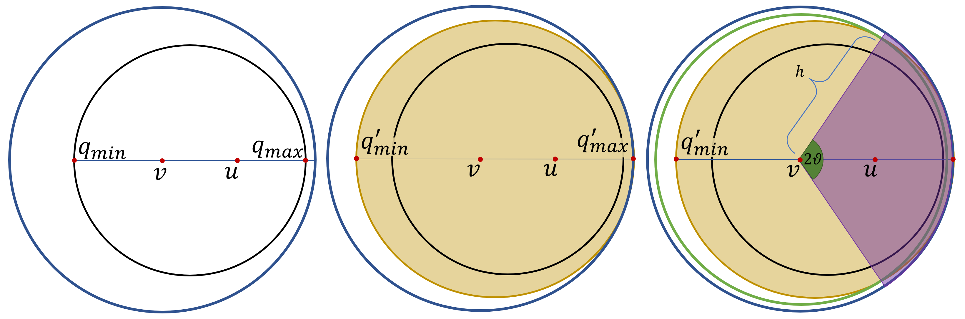
We recall that the hyperbolic disk is also a Euclidean disk . The Euclidean center must lie on the -axis (an easy way to see this is that reflection in the -axis is a -isometry that leaves invariant). Let and be the points where the circle intersects the -axis. See Figure 8, left. (So the Euclidean center of is the midpoint between these two points.) Since we have . As the points lie on the -axis, which is a hyperbolic line, we have
giving
By (1) it follows that . In other words, .
We set
and let
be the Euclidean disk with center and radius . Put differently, is the disk with on its boundary, that meets the -axis at a right angle at both points. This is not a hyperbolic disk (it is what is called a horocycle), but we do have that . See Figure 8, middle.
Let be the part of that is not contained in the sector . Then
since all points of are at least some positive Euclidean distance away from the boundary of the unit disk. See Figure 8, right. Evidently we have
as desired. (Note that depends only on and .)
Proof of Proposition 10. We let and be large constants, to be determined in the course of the proof. Let , be an arbitrary -tree, an arbitrary edge and an arbitrary vertex.
We first assume that . Then by Proposition 8, assuming without loss of generality we have chosen sufficiently large. And, assuming was chosen appropriately, by Proposition 9 we have
where is as provided by the proposition.
By Lemma 15, provided we chose appropriately, we have
Applying Lemma 12, provided we chose sufficiently large, we have
Let us thus consider the situation when . In this case we can apply Lemma 16 to show that, provided we chose and appropriately large,
This concludes the proof.
3.2 The upper bound
Here we will show the following proposition, which constitutes half of our main result.
Proposition 17
For every , there exists a such that for all , we have .
In order to prove this, we add the origin to the Poisson point process and colour it black, and consider the black component of in the Delaunay graph for . It suffices to show that, when and is sufficiently small, with positive probability the origin will be in an infinite black component. This is because all edges not involving the origin are also in the Delaunay graph for , and the origin a.s. has only finitely many neighbours (by Isokawa’s formula), so if the origin is in an infinite component then removing the origin may split its component into several components but at least one of these will be infinite.
For and we define the region
We choose to use the notation because the region is shaped like the letter C, at least for some choices of the parameters. See Figure 9.
Given and we define and by:
| (11) |
We point out that the probability distribution of does not depend on the choice of and (as long as they are distinct – otherwise the definition does not make sense).
Proposition 18
For every there exist and such that, for all and , the size of the black cluster of stochastically dominates the size of a Galton-Watson branching process with offspring distribution .
Proof. We can assume without loss of generality (otherwise by definition, and the theorem holds trivially). We set be a small constant to be determined during the course of the proof, let be as provided by Proposition 10, and we let be a large constant, to be determined more precisely during the course of the proof.
We consider an “exploration process” that iteratively constructs a -tree rooted at the origin. Recall that will be chosen larger than . At every iteration there will be a (finite) number of nodes, some of which are explored and some unexplored. The node having been explored means that all children of have already been added to the tree.
For each iteration , let denote the tree we have constructed at the end of iteration . We let denote the set of nodes of that have been explored at the end of iteration and be the set of nodes in that have not yet been explored; and we set .
If in any iteration there are no unexplored nodes, i.e. , then the construction of the tree stops and the final result is . Otherwise, if in each iteration we always have at least one unexplored node, then we continue indefinitely in which case of course .
In the first iteration we add the set defined above to the tree, as the children of the origin. To be more precise we define by . We set . In particular, the number of children of the origin will be .
In any subsequent iteration , assuming (otherwise the construction process will have finished), we pick an arbitrary unexplored node , and we denote by its parent in . The children of will be , and we let denote the number of children of . We update by defining via , and setting .
We point out that, since clearly is a -tree, it follows from Proposition 8 that we do not include any point twice (put differently that for all ), provided was chosen sufficiently large.
It remains to see that the size of the tree constructed via this process dominates the size of a Galton-Watson tree with offspring distribution . In order to do this, we will first establish that are independent, and then that are i.i.d. and finally that stochastically dominates .
We will consider, for each iteration , a (random) region that will be revealed by the exploration process during the -th iteration. Here we mean by “reveal” that the exploration process will use information about in order to determine , but – crucially – after the -th iteration the exploration process will not have uncovered any information on the status of the Poisson point process outside of .
We define by
setting so that the definition also applies for . We let be the tree on vertex set , rooted at and where the children of are for each . Clearly is also a -tree for each .
Given and , we can determine by revealing the status of the Poisson process inside . In order to now determine we need to determine, for each whether and there exists a disk such that and . Any such is contained in . Hence, given and , we can determine by revealing the status of the Poisson process inside the region
By Proposition 10 (applied to the tree consisting of a single edge ) and the choice of , we have
for all . It follows that
| (12) |
(We point out that the arguments giving (12) also apply to the case when , showing that is determined completely by .)
On the other hand, we also have
for every . Hence
| (13) |
where we apply Proposition 10 in the last line, and we assume we chose sufficiently large.
Moreover, for , by construction of the exploration process we have
Hence, for , given , the random set is completely determined by where
(For it might be the case that contains point of . So we cannot say that is completely determined by . It is however completely determined by .)
We consider an isometry satisfying and that lies on the positive -axis. Thus
and of course .
Since does not not intersect the areas revealed by previous iterations and it is isometric to for each , we find that are independent, and for in fact
(We write and not since .)
If were i.i.d. then would be a Galton-Watson tree with offspring distribution . In our case, we can describe the situation by saying the tree consists of a root attached to independent copies of a Galton-Watson tree with offspring distribution . We also point out that the sequence completely determines the size of the tree , via
(See for instance Sections 1.5 and 1.6 of [20]. Note that while the discussion there focuses on i.i.d., the above equation holds much more generally. See the remark following Definition 1.14 in [20].)
To conclude the proof, we note that, provided we chose sufficiently large, . Therefore, any point of in can only “prevent” the formation of edges between and some . In particular, for any we have
which gives
In other words, stochastically dominates . By Strassen’s theorem ([40]; an elementary proof of the version we need can for instance be found in Section 2.3 of [47]) there is a coupling of the sequence and an i.i.d. sequence such that for all and almost surely. The sequence can be used to generate a Galton-Watson tree with offspring distribution . We have . Hence, (under the coupling, almost surely) . In particular the size of the black cluster of the origin (which is at least ) stochastically dominates . This is what needed to be shown.
Having established Proposition 18, in order to prove Proposition 17 it suffices to show that, for sufficiently small and , there is a choice of such that ( with as specified in Proposition 18, and) . More specifically, we’ll keep (and ) constant, but we’ll let depend on .
We break the argument down in a series of relatively straightforward lemmas.
Lemma 19
For every and all the following holds, setting . Writing
we have
Proof. If then clearly almost and we are done. So we can assume . Clearly
using that for , and the choice of .
Lemma 20
For every and all the following holds, setting and letting be an arbitrary (fixed) point. Writing
we have
Proof. Clearly
as before using that and the choice of .
Lemma 21
For every and all the following holds, setting . Writing
we have
Proof. By Corollary 5:
where is as given by (2) and
In other words
using rotational symmetry of the hyperbolic area measure in the third line; that and the bound on in the fifth line; and the choice of in the last.
Lemma 22
For every and all the following holds, setting . Writing
we have
Proof. Applying Corollary 5 again, we have
where is given by (2) and this time
In other words
again using that and the choice of .
Lemma 23
There exists a such that, for all , all and all , the following holds, setting . Writing
we have
In the proof we’ll make use of the following definition and observations, that we’ll reuse later. For the Gabriel disk is the disk whose center is the midpoint of the hyperbolic line segment between and and whose radius is half the hyperbolic distance between and . Put differently, among all disks that have both and on their boundary, is the one of smallest hyperbolic radius.
The name “Gabriel disk” is in reference to the Gabriel graph, an object that has received some attention in the discrete and computational geometry literature. The Gabriel graph associated with a point set is the subgraph of the Delaunay graph whose edges are all pairs for which the Euclidean disk whose center is the midpoint between and and whose radius is half their distance contains no other points of .
The hyperbolic line segment between and splits into two parts of equal hyperbolic area. We shall denote by the part that is on the left as we travel from to along the hyperbolic line segment, and by the one that is on the right. See Figure 10.
We’ll repeatedly make use of the following straightforward observation.
-
()
For all and every disk such that , we have either or (or both).
(This is easily seen by applying a suitable isometry that maps to the -axis and their midpoint to the origin, so that are mapped to ordinary, Euclidean half-disks – as in Figure 10.)
In light of observation (), in order to prove Lemma 23 it suffices to prove the following statement, which we separate out as a lemma for convenient future reference.
Lemma 24
There exists a such that, for all , all and all , the following holds, setting . Writing
we have
Proof of Lemma 24. We let be a small constant, to be determined in the course of the proof. By Corollary 5
where is again given by (2) and
We have
where in the last line we use that was chosen sufficiently small; that as so that for sufficiently large; that ; and that .
Switching to hyperbolic polar coordinates (i.e. ) we find
using the substitution (so that ) in the third line
Lemma 25
There exists a such that for all , all and all the following holds, setting . Writing
we have
In the proof we’ll make use of the following definition and observations, that we’ll reuse later. For and with , there exist precisely two disks such that and . We let denote the union of these two disks. (The notation stands for “double disk”.) The hyperbolic line segment between and splits into two parts of equal hyperbolic area. We denote by the part that is on the left as we travel from to along the hyperbolic line segment between them, and by the part on the right. See Figure 11.
Another observation that we’ll use repeatedly is:
-
()
For all and and every hyperbolic disk such that and , we have either or (or both).
(Again this is easily seen by applying a suitable isometry that maps to the -axis and their midpoint to the origin, as in Figure 11. Fact 2 ensures that the image of the hyperbolic disk is a Euclidean disk with the images of on its boundary.)
In light of observation (), in order to prove Lemma 25 it suffices to prove the following statement, which we separate out as a lemma for convenient future reference.
Lemma 26
There exists a such that for all , all and all the following holds, setting . Writing
we have
where is as given by (2). Next we point out that, by symmetry
where the last inequality holds provided we chose sufficiently large, since and as .
Hence
using the choice of .
We are now ready to prove the following statement.
Proposition 27
For every there exist such that the following holds. For every there exists a such that, for all , setting and , we have that
(With as defined in (11).)
Proof. As pointed out right after the definition of , its probability distribution is the same for any choice of . For definiteness we take and . We let be an arbitrary constant. We let be large constants, and a small constant, to be determined in the course of the proof.
Let us denote by the number of black cells adjacent to the typical cell. (Recall that “typical cell” refers to the cell of the origin in the Voronoi tessellation for .) By Isokawa’s formula
using the choice of in the inequality. Next, we point out that
with – as defined in Lemmas 19–25. Applying these lemmas we see that, provided we chose sufficiently small,
where the second inequality holds provided we chose the constant sufficiently large and the constants sufficiently small. (To be more explicit : we can for instance first choose such that and then we choose such that and finally choose such that – and at the same time is small enough so that Lemma 23 and 25 apply.)
3.3 The lower bound
Here we will show the following proposition, which constitutes the remaining half of our main result.
Proposition 28
For every , there exists a such that for all , we have .
In the proof of Proposition 17 we could in a sense afford to “ignore” some adjacencies in the Voronoi tessellation. The supercritical Galton-Watson tree we constructed in the proof of Proposition 18 uses only adjacencies of convenient lengths and is such that if two edges share an endpoint, the angle they make is not too small.
Now we need to show that no infinite black component exists almost surely, for sufficiently small and . We cannot a priori exclude the possibility that an infinite component exists but every infinite connected subgraph contains (has to contain) “unusual” edges. In particular, a hypothetical infinite component might exist that does not contain an infinite -tree.
To make our life easier, we adopt a more generous notion of adjacency, in the form of pseudopaths.
Definition 29
Given parameters , we say a (finite or infinite) sequence of distinct points is a pseudopath (wrt. and ) if one of the following holds for each :
-
I
and one of the following holds. There exists a disk such that and , or; , or; .
-
II
;
-
III
and ;
-
IV
and either , or , (or both).
(Of course the demand that in I only applies when , and similarly the case III can only occur when .) The length of a finite pseudopath is , the number of points minus one, and we use the term pseudo-edge for a consecutive pair of points on a pseudopath. In particular pseudopaths of length one are pseudo-edges, but not all pseudo-edges are pseudopaths of length one (because of III which can only apply when the pseudopath has length ). As in the case of ordinary paths, we denote by the set of vertices of the pseudopath .
With each pair of points of a pseudopath we associate a “certificate” . This will be a region such that in order to verify that is a pseudo-edge, in addition to the location of the previous point of the pseudopath if is part of a pseudopath of length , only is relevant. Specifically, we set
(Note that if and is a disk with and then . Also note that if then .) For notational convenience we also set
for every sequence .
Pseudo-edges of type I will be called good, and all other types of pseudo-edges are bad. A pseudopath is good if all its pseudo-edges are good.
A finite pseudopath is called a chunk if the final pseudo-edge is bad and all other pseudo-edges are good. So a chunk can for instance consist of a single bad pseudo-edge.
Definition 30
A linked sequence of chunks is a (finite or infinite) sequence of chunks such that
-
(i)
if , and;
-
(ii)
For each , writing and , we have
and in addition one of the following holds:
-
a)
, or
-
b)
and , or
-
c)
and .
-
a)
We’ll say a linked sequence of chunks is infinite if the sum of the lengths of the chunks is infinite. In other words, an infinite linked sequence of chunks either consists of infinitely many finite chunks, or consists of finitely many chunks of which the last chunk has infinite length.
Proposition 31
For every and , almost surely, one of the following holds.
-
(i)
The black component of in the Voronoi tessellation for is finite, or;
-
(ii)
There is a black, infinite, good pseudopath, or;
-
(iii)
There is a black, infinite linked sequence of chunks starting from .
For clarity, we emphasize that the infinite pseudopath mentioned in item (ii) does not need to contain the origin .
Our strategy for the proof of Proposition 28 is of course to show, after having established Proposition 31, that there is a choice of such that, for all small enough and all , almost surely options (ii) and (iii) of Proposition 31 do not occur. This will imply that the black component of the origin in the Voronoi tessellation for is a.s. finite. A short argument will then show this also implies that, almost surely, all black components in the Voronoi tessellation for are finite.
For the proof of Proposition 31 we will use the following observation that is a straightforward consequence of the Slivniak-Mecke formula and Isokawa’s formula. We provide a proof for completeness.
Lemma 32
For every and , almost surely, every Voronoi cell is adjacent to a finite number of other Voronoi cells.
Proof. Let us write
By the Slivniak-Mecke formula
where is as given by (2) and with denoting the degree of in the Delaunay graph of . By symmetry considerations, for every (fixed) we have
where denotes the typical degree and we apply Isokawa’s formula. It follows that, for every :
Hence also , which implies that almost surely.
We’ll also need the following observation in the proof of Proposition 31.
Lemma 33
For every , almost surely, for every the number of pseudo-edges with for which is finite.
Proof. Fix an arbitrary . Clearly the number of pseudo-edges with for which and is bounded by where . Since , the random variable is finite almost surely.
Pseudo-edges not counted by must satisfy and hence and either or (or both). By symmetry considerations, it suffices to count
For each pair counted by there is an such that . We must also have that , since and .
Writing
we thus have
Applying the Slivniak-Mecke formula, we find that
where is as given by (2) and
For every have
for a suitably chosen small constant . (The last step in some more detail : for all for which , we have . Since as , there is an such that for all . We can now choose a small such that for all .) It follows that
and hence
So is finite almost surely.
We have now shown that for every fixed we have where
Since whenever we also have
which is what needed to be shown.
Proof of Proposition 31. We fix arbitrary and . Since the typical degree has finite expectation by Isokawa’s formula, almost surely, the cell of the origin in the Voronoi tessellation for is adjacent to at most finitely many other cells. For every point of , the number of cells it is adjacent to in the Voronoi tessellation for is at most one more than the number of cells it is adjacent to in the tessellation for . In particular, by Lemma 32, also in the Voronoi tessellation for , almost surely, each cell is adjacent to at most finitely many other cells.
We consider an arbitrary realization of the Poisson process (in other words, a locally finite point set , partitioned into two parts ) for which each Voronoi cell of is adjacent to finitely many others, and such that, for every , the ball intersects at most finitely many certificates of pseudo-edges. We will show that in such a realization either the black cluster of the origin is finite, or there exists an infinite, good, black pseudopath, or there exists an infinite linked sequence of chunks all of whose points are black (or more than one of the three options occurs).
Suppose thus that the origin lies in an infinite black component (otherwise we are done). Since each cell is adjacent to finitely many others, there must exist an infinite (ordinary) path with and (distinct). This is of course also a pseudo-path. If only finitely many pseudo-edges of are bad then we are done, as will contain a black, infinite, good pseudopath. Hence from now on we will assume that has infinitely many bad edges. In particular, we can find a such that the pseudo-edges are good and is bad. We set .
Let us say that an index interacts with a subpath of if one of the following holds: or or .
We now let be the largest index that interacts with . That exists (is finite) follows from the fact that
for some . Since contains infinitely many bad pseudo-edges, there exists a such that the pseudo-edges are good and is bad. We set . (A minor subtlety needs to be added here. When we say is bad, we mean that it is bad wrt. the path . We do this in order to handle the case where is a type III pseudo-edge of . If we took this single pseudo-edge as the path , then would not be a chunk but a good pseudopath.)
We now let be the largest index that interacts with . Again exists as is contained in for some . Since contains infinitely many bad edges, there exists such that the pseudo-edges are good and is bad (wrt. the path ). We set .
We continue defining and and analogously, producing an infinite linked sequence of chunks .
(We point out that the choice of guarantees that no index interacts with any of while interacts with but not . From this it easily follows that the demands (i), (ii) of Definition 30 are met.)
Since we considered an arbitrary realization of that satisfies two conditions that both hold almost surely, it follows that almost surely either the black cluster of the origin is finite or there exists an infinite linked sequence of chunks starting from the origin all of whose points are black.
The main thing that now remains, in order to prove Proposition 28, is to show that for a suitable choice of and for sufficiently small and with a small constant, almost surely there is no black, infinite, good pseudopath and no black, infinite linked sequence of chunks starting from .
As in the proof of the upper bound, from now on we will always take . The parameters will be constants that depend on and that we will choose appropriately in the end. We will use an inductive approach bounding the expected number of good pseudopaths, respectively linked sequences of chunks, of length starting from the origin. With this in mind, we will prove a number of lemmas designed to deal with the different ways in which an additional point can be added to an existing good pseudopath, respectively linked sequence of chunks, of length . But, first we need to derive some additional facts about hyperbolic geometry. Again, when reading the paper for the first time, the reader may wish to only read the definitions and lemma statements and skip over the proofs.
3.3.1 More geometric ingredients
Let us say that a sequence of points is a pre-chunk (wrt. ) if they are placed in such a way that they will form a chunk whenever the random point set turns out favourably. That is, is a pre-chunk if for and for all and in addition or or and . In particular, a pre-chunk is such that forms a -path with .
If and (in case ) for then we speak of a good pre-pseudopath.
The first geometric observation in this section will be helpful for the situation when we want to add a new pseudo-edge to an existing pseudopath, and will also be used by later proofs in this section. It tells us that if we want to add a new pseudo-edge to a good pre-pseudopath, then either the intersection of the certificate of the new pseudo-edge and the certificates of the existing path is contained in a ball of constant radius (and hence has rather small area), or the new edge makes a small angle with the last edge of the existing pseudo-path. This will translate into useful bounds once we start estimating the expected number of linked sequences of chunks later on.
Lemma 34
For every there are and such that the following holds for all . If is such that is a good pre-pseudopath wrt. then either
or
(or both).
Before giving the proof, we point out that by setting we obtain:
Corollary 35
For every there are and such that the following holds for all . If is a good pre-pseudopath (wrt. ) then
Proof of Lemma 34. We fix . For any , if is a pre-chunk wrt. then is a -path, setting . We also point out that, since is a good pre-pseudopath, for . By Proposition 10 there exist constants and such that, whenever , we have
Let us write . By Lemma 16 (applied with ), we can assume without loss of generality that the constant is such that:
Since , we have that if then . It follows that either or , as claimed.
Our next observation provides an upper bound on the number of edges in a pseudopath whose certificates intersect a given ball. This will be of use to us later on several times, for instance when we want to estimate or bound the expected number of pseudo-edges that can act as the start of a new chunk extending a given sequence of chunks.
Lemma 36
For every there exists such that, for every , every pre-chunk and every ball , it holds that
Proof. By Proposition 9 and the remark following the definition of pre-chunk, there exists an such that if and then
for all sufficiently large and all .
For , let us denote by the centers of the two disks whose union is . If then
(the second inequality holding for sufficiently large).
Now observe if and only if . So if and then
the first inequality holding provided was chosen sufficiently large. Rearranging, we find
This shows that the number of such that is at most . Including also , we obtain which is smaller than the bound in the statement of the lemma.
Using the previous lemma, we can now show that, for any ball whose radius is only a constant larger than (the radius of the two balls whose union is the certificate of a good pseudoedge), most of the area of the ball lies outside the certificate of any given pseudopath.
Lemma 37
For every there exists such that, for every , every good pre-pseudopath and every ball with radius , it holds that
Proof. We let be a large constant, to be chosen more precisely during the proof.
By Lemma 36, we have
As , we have, provided we chose sufficiently large, that . Hence
Since the RHS is decreasing in for , we have
provided we chose sufficiently large.
Next we present another observation that will be helpful for the situation when we want to add a new pseudo-edge to an existing pseudopath. It tells us that one of three things must happen, each of which will translate into useful bounds once we start estimating the number of linked sequences of chunks later on.
Corollary 38
For every there exists such that, for every and every pre-chunk wrt. we have that either
or
or
(or more than one of the above hold).
Proof. We let be a large constant, to be determined in the course of the proof and we let be arbitrary and we let be an arbitrary pre-chunk wrt. .
Of course there is nothing to prove if . If then has radius and we are done by Lemma 37 – assuming without loss of generality we chose larger that the bound provided in that lemma.
Let us thus assume . By Lemma 34, there are constants such that if then either
or
In the latter case we are clearly done. In the former case we note that
provided was chosen sufficiently large.
For some of the remaining proofs needed for the lower bound, we’ll use the following notion which may be of independent interest. For sets we let
The abbreviation stands for “asymmetric Hausdorff distance”. As the reader may already have recognized, the Hausdorff distance between equals .
The next two lemmas are a preparation for the third one, Lemma 41. That lemma allows us to bound the area of intersection of a given ball with the certificates of a given (pre-)pseudopath. This will be of use to us when we estimate the expected number of linked sequences of chunks later on.
Lemma 39
For every there exists an such that the following holds. Let be a disk and a hyperbolic circle such that . Then we have .
Proof. The statement is obviously true if . Similarly it is also true if and intersect in a single point (the common point would line on the line joining and ). So from now on we can assume this is not the case.
Let denote the two intersection points of the circles and . It suffices to show that, provided and is sufficiently large, . For convenience we write . We next point out that
(To see this we first note that by the triangle inequality for all . In other words, for all . Applying a suitable isometry if needed, we can assume without loss of generality that is the origin and lies on the negative -axis. The point satisfies , as lies on the -axis which is a hyperbolic line.)
By the hyperbolic law of cosines,
Hence
The statement follows by taking .
Lemma 40
We have
Proof. It suffices to show that for every there exists such that implies that . We thus let be a large constant, to be determined in the course of the proof, and we let be arbitrary disks with .
If then and are disjoint and we are done. For the remainder of the proof, we therefore assume .
Each of the circles with satisfies . Applying Lemma 39, having chosen sufficiently large, we can assume that for all . It follows that
Next we note that, by rotational symmetry of the hyperbolic area measure
| (14) |
We also have
| (15) |
where the second inequality follows from the fact that is decreasing in for and the last inequality holds provided we chose sufficiently large, and uses that as .
provided we chose sufficiently large. This clearly implies the statement of the lemma.
Lemma 41
For every there exist such that, for every pre-chunk and every disk with we have
Proof. We fix a large constant , to be determined more precisely during the course of the proof. For convenience we’ll write and . We let be the balls that feature in the definition of . That is each is either or a disk of diameter with for some . In particular and .
By Lemma 40 we can take the constant such that the assumption that implies that for each .
We set . If then the statement clearly holds. For the remainder of the proof we thus assume .
By Lemma 36, assuming was chosen sufficiently large, we have (each certificate is either a single ball or the union of two balls). Hence, provided we chose and sufficiently large, implies . We have
the last inequality holding assuming we have chosen and sufficiently large. Next we point out that
provided and were chosen sufficiently large, using in the second line that as ; in the third line that is decreasing for ; and in the last line that as (for every ). It follows that if then also
as claimed.
We conclude this subsection, with two lemmas giving conditions under which hyperbolic angles are small. Again, we will use these when estimating the expected number of linked sequences of chunks later on.
Lemma 42
There is a universal constant such that the following holds. If and are such that then either or .
Proof. Let be as provided by Lemma 11. For notational convenience we write and .
The disks and intersect if and only if . If then Lemma 11 tells us that . It follows that if and then .
Let us then assume . If then the hyperbolic cosine rule gives
where we have used that for all . Rearranging and taking square roots gives .
We’ll use another rather straightforward consequence of the hyperbolic cosine rule:
Lemma 43
For all we have
Proof. For notational convenience, write and . It suffices to show that .
If then the hyperbolic cosine rule gives that
(Using that for in the third line.)
If on the other hand then similarly
3.3.2 Counting good pseudopaths
The next point of order is to bound the expected number of black, good pseudopaths starting from the origin. We plan to use an inductive approach and begin with a couple of lemmas designed for the situation where we add a good pseudo-edge to an existing, good pseudo-path.
Lemma 44
For every and there exist such that the following holds for all and all , setting .
Let be an arbitrary good pre-pseudopath and, writing , define
We have
Before proceeding with the proof, let us clarify that in the above lemma we also allow . In that case the demand of course does not apply.
Proof. We let be a small constant to be determined in the course of the proof, and take an arbitrary and . Once again we apply Corollary 5 to find that
where is again as given by (2) and this time
By Corollary 35, assuming was chosen sufficiently small, if is such that then .
Applying a suitable isometry if needed (which leaves the distribution of invariant), we can assume without loss of generality that is the origin. Recall that any disk satisfying and satisfies . So if is such that and then
where if is an edge of the Delaunay graph for and otherwise. It follows that
where the second line follows by Isokawa’s formula (and the Slivniak-Mecke formula to phrase the typical degree as an integral).
Since is a constant we have as . So, provided we chose sufficiently small, we have
as claimed.
Lemma 45
For every there exists a such that the following holds for all and all , setting .
Let be an arbitrary good pre-pseudopath and, writing , define
We have
Proof. The proof is nearly identical to the proof of the previous lemma. Reasoning as the proof of Lemma 44, there is a constant such that
for all sufficiently small , where is as in Lemma 26.
Since provided we chose sufficiently small, the result follows from Lemma 26
These last two lemmas allow us to prove the following statement using an inductive approach. Here and in the rest of the paper we write
Lemma 46
For every and there exists a such that the following holds for all and all , setting .
Proof. By Corollary 5 we have
| (16) |
where is as given by (2) and is the indicator function of the event that form a good pseudopath (wrt. the parameters and the point set ). We note that
| (17) |
where
Next, we note that if is not a good pre-pseudopath then and whenever is a good pre-pseudopath then
| (18) |
as and are independent; and the former determines the value of , while the latter determines .
| (19) |
for every such that is a good pre-pseudopath.
If is not a good pre-pseudopath then
.
Combining (16)–(19), we see that
The lemma follows by iterating the recursive inequality.
The previous lemma immediately gives that, provided we chose a sufficiently large constant (how large we need to take it depends on ), for all sufficiently small intensities , almost surely, there are no infinite, black, good pseudopaths starting from the origin. In fact something slightly stronger holds:
Corollary 47
For every there exists a such that for all and the following holds.
There exists a such that, when and , setting , almost surely there are no infinite, black, good pseudopaths.
Proof. As pointed out earlier, we can choose such that for all and there is a such that, whenever when and , almost surely there is no infinite, black, good pseudopath starting from the origin.
Let be arbitrary and write
By Corollary 5
where is given by (2) as usual and if and and there is an infinite, black, good, pseudopath (wrt. and the point set ) starting from ; and otherwise. If then by definition of , and if then
since the distribution of is invariant under the action of isometries of the Poincaré disk ( if is an isometry), and in particular under an isometry that maps to ; and we know that the origin a.s. is not on any infinite, back, good, pseudopath as remarked just before the statement of the lemma. It follows that and hence also a.s., for each separately. Thus
as whenever .
Recall that our strategy for the proof that for small is to prove that almost surely no black, infinite, good pseudopath and no black, infinite, linked sequence of chunks starting from the origin will exist (for an appropriate choice of and ). In the light of the last corollary, we now turn our attention to linked sequences of chunks.
3.3.3 Counting chunks starting from the origin
Next, we bound the number of black chunks starting from the origin. We will exploit our results on good pseudopaths, using that a chunk is just a good pseudopath with a single bad pseudo-edge stuck to the end. We begin with a few lemmas designed for adding a last, bad edge to an existing good pseudopath. The names of the random variables described by the lemmas are with some subscript, where stands for “last” and the subscript corresponds to the type of edge under consideration.
Lemma 48
For all there exist such that the following holds for all and all , setting .
Let be arbitrary, and set and
We have
for all .
Proof. We let be a small constant to be determined in the course of the proof, and take an arbitrary and . Without loss of generality (applying a suitable isometry if needed) we can assume is the origin.
If satisfies and then of course also
using that
(the term referring to the situation where tends to zero) and assuming that we have chosen sufficiently small (so that is large). Analogously we also have
for all such . By Corollary 5 and this last observation:
with given by (2).
Applying a change to hyperbolic polar coordinates to we find
Applying the substitution (so that ), we find
Corollary 49
For all there exist such that the following holds for all and all , setting .
Let be an arbitrary good pre-pseudopath, and set and
We have
for all .
Proof. We let be small constants to be determined in the course of the proof, and take an arbitrary and . Without loss of generality (applying a suitable isometry if needed) we can assume is the origin.
Since , by Corollary 38 with and , assuming we have chosen sufficiently small, we have
where is as defined in Lemma 48 above and
setting .
In particular if . In this case we are clearly done by Lemma 48.
To prove it also for , we also need to bound . Lemma 20 shows that
having chosen sufficiently small for the second inequality. (To be precise, having chosen .)
Adding the bounds on and proves the result for .
We will denote
and, for all :
Recall that denotes the number of black, good, pseudopaths starting from the origin of length .
Corollary 50
For every there exists a such that the following holds for all and , setting .
We have
| (20) |
| (21) |
and
| (22) |
for all .
where is given by (2) and is the indicator function that is a chunk (wrt. the point set ), whose last pseudo-edge is of type II.
Let denote the indicator function that is a good pseudo-path wrt. the point set . We have
It follows that
The proof of (21) is analogous, using the indicator function in place of , replacing with (for arbitrary) and using Lemma 20 in place of Lemma 19.
For the proof of (22), we use that if denotes the indicator function that form a chunk (wrt. ) whose last pseudo-edge has length then
where
Since and are independent for any choice of , we have
If do not form a good pre-pseudopath then . Otherwise we can apply Corollary 49 (and Corollary 5) to show that
In other words,
as desired.
3.3.4 Counting linked sequences of chunks
Next, we turn attention to counting the number of linked sequences of chunks. The first few lemmas are designed for dealing with the first pseudo-edge of a new chunk that will be linked to an existing chunk. The names of the random variables described in these lemmas are with some subscript, where stands for “first” and the subscript corresponds to the type of the new pseudo-edge to be added and the type of link under consideration. (The link types being a, b, c corresponding to the cases listed in part (ii) of Definition 30.)
Lemma 51
For every there exist such that the following holds for all and , setting .
Let be an arbitrary pre-chunk and define
Then we have
Proof. We can write with and balls whose radii are either or .
For we define
Observe that if then either equals or . In particular we have .
We see that
We can thus focus on bounding the individual expectations . For the moment, we pick some . Without loss of generality (applying a suitable isometry if needed) the center of is the origin . Applying Corollary 5 and a (double) switch to hyperbolic polar coordinates:
where
Note that implies that . Applying Lemma 43, we see that implies that . (Here and elsewhere for .) Therefore
It follows that
| (23) |
By symmetry considerations
(We have an inequality and not an equality to account for the possibility that .) Filling this back into (23), we obtain
using in the last line that , the diameter of , is either or . Adding the bounds on and using the inequality gives
as claimed in the lemma statement.
Lemma 52
For every there exist such that the following holds for all and , setting .
Let be an arbitrary pre-chunk and define
Then we have
Proof. As usual, we let be a small constant, to be determined in the course of the proof. As in the previous proof, we write with and balls whose radii are either or . Let us write . By Corollary 5
where is the “typical degree” as given by (8), is as defined in Lemma 19 and as defined in Lemma 26, and; we apply Isokawa’s formula (Theorem 6) and Lemmas 19 and 26 and we use that and that for all to obtain the fourth line. In the fifth line we use that and in the last line that we chose sufficiently small (so that is large).
Lemma 53
For every there exist such that the following holds for all and , setting .
Let be an arbitrary pre-chunk and write and
Then we have
for all .
Proof. The demand that implies that
as well. Provided is sufficiently small (so that is sufficiently large), Lemma 41 (with ) implies that
The result now follows from immediately Lemma 48.
Lemma 54
For every there exist such that the following holds for all and , setting .
Let be an arbitrary pre-chunk and write and
Then we have
for all .
Proof. As usual, we let be a small positive constant, to be determined during the course of the proof, and we fix an arbitrary , and .
We can write with and balls whose radii are either or .
For we define
and we point out that
In particular it suffices to bound each expectation separately. For the moment we fix . Applying a suitable isometry if needed, we assume without loss of generality that the center of is the origin.
By Corollary 5:
with given by (2) and
Applying a change to hyperbolic polar coordinates to we find
| (24) |
Next, we consider the inner integral for some (fixed for the moment) satisfying . Let be a hyperbolic isometry that maps to the origin and to the negative -axis. (So that .) Note that
where
We point out that if then it must certainly hold that . By Lemma 42, using that by assumption, we must also have that
We see that
Since , we certainly have
Assuming was chosen sufficiently small, we can apply Lemma 41 to see that
and hence
where the last inequality holds assuming we chose sufficiently small, and assuming that (and using ). Completely analogously, as well.
We see that
Applying (7), we find
Changing to hyperbolic coordinates, i.e. gives
We next apply the substitution (so that ) to obtain
using in the last line that and .
Filling this back into (24) we find
using that and in the third line.
Now
| (25) |
using that .
We also have
| (26) |
using the substitution in the second line, the substitution in the third line and that . Adding (25) and (26) and multiplying by gives the result.
Lemma 55
For every there exist such that the following holds for all and , setting .
Let be an arbitrary pre-chunk and write and
Then we have
for all .
Proof. As usual, we let be a small constant, to be chosen appropriately during the course of the proof. Writing and applying Corollary 5, we have
applying Lemma 24. Next we remark
the last inequality holding provided we chose sufficiently small.
Recall that denote the number of black chunks starting from the origin, with length and final pseudo-edge of type II, respectively type III, respectively type IV and final pseudo-edge of length .
We now need to introduce analogous notations to deal with linked sequences of chunks. We set
We let and be defined analogously. Of course
| (27) |
In particular, Corollary 50 provides bounds on the expectations and when . The next lemma provides a system of recursive inequalities that will allow us to also bound these expectations for . From now on, it will be convenient to assume the parameter is an integer. Note that so far the only result that puts any restrictions on the value of is Corollary 47 which just states it has to be taken sufficiently large.
Lemma 56
For every and there exists a such that for all and , setting , the following holds.
For all , writing
we have
and
for one of or with , and for all when and all otherwise.
Proof. We’ll need to introduce even more notation. We let
denote the possible types of the final pseudo-edges of chunks, respectively types of links between consecutive chunks – corresponding to the cases described in part (ii) of Definition 30.
For and we write for the number of black, linked sequences of chunks starting from , such that has length and final pseudo-edge of type (for all ), and such that the link between and corresponds to case of part (ii) of Definition 30 (for ). Clearly we can write for each and :
| (28) |
We will first derive the last inequality claimed in the lemma statement. Let us fix and such that either in case or in case . We pick vectors satisfying and .
The parameters determine the number of vertices in any of the linked sequences of pseudopaths counted by . For any such sequence of pseudopaths we have with and . (To be precise as for all but every time the last vertex of coincides with the first vertex of .) By Corollary 5 we can write, for as determined by the parameters
where is given by (2) and is the indicator function that form a linked sequence of pseudopaths of the required kind wrt. the point set .
The vertices of are . If then is both the first vertex of and also the last vertex of . Recall that needs to be disjoint from (and this set is completely determined by ), otherwise will equal zero. So, provided we can write, for every :
| (29) |
where is the indicator function that forms a chunk of length and with final edge of type (with respect to the point set ). Here we use that unless the position of is such that for ; and if are such that all these intersections are empty then the event that and the event that are independent.
We can write
| (30) |
For every fixed , applying an isometry that maps to and Corollary 5, we have
| (31) |
Of course, for every fixed , we have
by Lemma 20. It follows that:
| (32) |
(Provided .)
If then , the first vertex of , does not lie on and we need that and intersects . So instead of (29) we can now write
| (33) |
For any fixed we have that if is not a pre-chunk then and otherwise we can apply Lemma 51 to get
where if and otherwise is determined via . (That is, if for some then .) We conclude that if then
| (34) |
If then we replace (33) with
| (35) |
| (36) |
(Provided .)
establishing the last inequality in the lemma statement.
The first inequality (the case when and ) follows analogously, replacing in (29), (33), (35) by and applying Lemma 20 to the innermost integral in the analogues of (30).
The second inequality (the case when and ) follows in the same way, now using the indicator function that and and applying Lemma 21.
For the case when and we replace by the indicator function corresponding to from Lemma 53 in case ; by the indicator function corresponding to from Lemma 54 in case ; and the indicator function corresponding to form Lemma 55 in case ; and then apply Lemma 53, respectively Lemma 54, respectively Lemma 55 to the innermost integral in the analogues of (30).
Lemma 57
For every and there exist and such that and for all and , setting , almost surely there are no infinite, black, linked sequences of chunks starting from the origin .
Proof. We will make use of the bounds provided by Lemma 46, Corollary 50 and Lemma 56. We will choose the integer so large that . So in particular, for sufficiently small, the expected number of good, black pseudopaths starting from the origin satisfies
The recursive relations given by Lemma 56 show that for all :
For the sake of the presentation, we introduce an additional small constant . Without loss of generality we can assume chose large enough so that
We can also assume are such that . Filling these bounds into the bound on gives
the last line holding because we have chosen appropriately.
To recap, we can choose in such a way that for all ; and . In particular as .
Let us denote by the total number of black, linked sequences of chunks starting from the origin and consisting of precisely chunks. Obviously
But then we also have that
It follows that, almost surely, there are is no infinite, black, linked sequence of chunks starting from .
Corollary 58
For every there is a such that for all and all , almost surely, the black cluster of in the Voronoi tessellation for is finite.
Proof of Proposition 28. This follows from Corollary 58 by a near verbatim repeat of the proof of Corollary 47. We only mention the changes that need to be made. Now, we let be the number of that are part of an infinite black component of the Voronoi tessellation, and we let be the indicator function that and that lies in an infinite, black cluster in the Voronoi tessellation for .
4 Suggestions for further work
Our Theorem 1 states that as , answering a question of Benjamini and Schramm [9]. A natural direction for research is to try and find more terms in the expansion.
Problem 59
Determine a constant such that as , or show no such constant exists.
In our proofs we have either taken , for the upper bound on , or , for the lower bound. We have always taken constant in our paper and have not made any effort to see how fast we can send to zero as a function of before our proof technique breaks down. Of course many of our bounds are rather crude and it seems likely that more fine-grained proof techniques will need to be developed.
As mentioned in the introduction, the critical value for percolation in for high dimension is related, at least on an intuitive level, to our result. And, as also mentioned, a trivial comparison to branching processes shows the critical value for bond percolation on satisfies , the reciprocal of the degree. (It was in fact shown by Van der Hofstad and Slade [48] that . So we even have for large enough .) Inspired by this, and the fact that the typical degree is actually strictly larger that , we offer the following conjecture:
Conjecture 60
There exists a such that for all .
Of course the answer to Problem 59 is likely to also tell us whether this conjecture holds or not. But, perhaps Conjecture 60 can be settled via a different route.
We reiterate a natural conjecture of Benjamini and Schramm.
Conjecture 61 ([9])
is strictly increasing.
Another natural conjecture in the same vein is:
Conjecture 62
is differentiable.
We were tempted to write “smooth” in place of “differentiable”, but opted against it to give whoever attempts to prove the conjecture the best chances.
Of course Poisson-Voronoi percolation can also be defined on -dimensional hyperbolic space , and we expect that the main result of the current paper will generalize. In two dimensions, the typical degree is the same as the number of -faces of the typical cell. In -dimensions the relevant corresponding quantity is the number of -faces of the typical cell.
Conjecture 63
For every , as the intensity , the critical value for Poisson-Voronoi percolation on is asymptotically equal to the reciprocal of the expected number of -faces of the typical cell.
It might be possible to leverage some of the existing work on the expected -vectors of the typical cell in [13, 19, 26]. But, of course it might also be possible to prove or disprove the conjecture without knowing the expected number of -faces precisely.
In a recent separate paper, we proved the conjecture of Benjamini and Schramm that as for planar, hyperbolic Poisson-Voronoi percolation. It seems natural to expect that this result generalizes to arbitrary dimensions.
Conjecture 64
For every , as the intensity , the critical value for Poisson-Voronoi percolation on tends to the critical value for Poisson-Voronoi percolation on .
Acknowledgements
We thank the anonymous referee for many helpful comments that have greatly improved the paper.
References
- [1] D. Ahlberg and R. Baldasso. Noise sensitivity and Voronoi percolation. Electron. J. Probab., 23:Paper No. 108, 21, 2018.
- [2] D. Ahlberg, S. Griffiths, R. Morris, and V. Tassion. Quenched Voronoi percolation. Adv. Math., 286:889–911, 2016.
- [3] P. Balister and B. Bollobás. Bond percolation with attenuation in high dimensional Voronoĭ tilings. Random Structures Algorithms, 36(1):5–10, 2010.
- [4] P. Balister, B. Bollobás, and A. Quas. Percolation in Voronoi tilings. Random Structures Algorithms, 26(3):310–318, 2005.
- [5] I. Benjamini, J. Jonasson, O. Schramm, and J. Tykesson. Visibility to infinity in the hyperbolic plane, despite obstacles. ALEA Lat. Am. J. Probab. Math. Stat., 6:323–342, 2009.
- [6] I. Benjamini, Y. Krauz, and E. Paquette. Anchored expansion of Delaunay complexes in real hyperbolic space and stationary point processes. Probab. Theory Relat. Fields, to appear. Available from https://doi.org/10.1007/s00440-021-01076-y.
- [7] I. Benjamini, E. Paquette, and J. Pfeffer. Anchored expansion, speed and the Poisson-Voronoi tessellation in symmetric spaces. Ann. Probab., 46(4):1917–1956, 2018.
- [8] I. Benjamini and O. Schramm. Conformal invariance of Voronoi percolation. Comm. Math. Phys., 197(1):75–107, 1998.
- [9] I. Benjamini and O. Schramm. Percolation in the hyperbolic plane. Journal of the American Mathematical Society, 14(2):487–507, 2001.
- [10] B. Bollobás and O. Riordan. The critical probability for random Voronoi percolation in the plane is 1/2. Probability theory and related fields, 136(3):417–468, 2006.
- [11] B. Bollobás and O. Riordan. Percolation. Cambridge University Press, 2006.
- [12] S.R. Broadbent and J.M. Hammersley. Percolation processes. I. Crystals and mazes. Proc. Cambridge Philos. Soc., 53:629–641, 1957.
- [13] P. Calka, A. Chapron, and N. Enriquez. Poisson-Voronoi tessellation on a Riemannian manifold. Int. Math. Res. Not. IMRN, (7):5413–5459, 2021.
- [14] J.T. Cox and R. Durrett. Oriented percolation in dimensions : bounds and asymptotic formulas. Math. Proc. Cambridge Philos. Soc., 93(1):151–162, 1983.
- [15] H. Duminil-Copin, A. Raoufi, and V. Tassion. Exponential decay of connection probabilities for subcritical Voronoi percolation in . Probab. Theory Related Fields, 173(1-2):479–490, 2019.
- [16] L. Flammant. Hyperbolic radial spanning tree. Preprint, available from arXiv:2012.03467.
- [17] M.H. Freedman. Percolation on the projective plane. Math. Res. Lett., 4(6):889–894, 1997.
- [18] E. N. Gilbert. Random plane networks. J. Soc. Indust. Appl. Math., 9:533–543, 1961.
- [19] T. Godland, Z. Kabluchko, and C. Thäle. Beta-star polytopes and hyperbolic stochastic geometry. Preprint, available from arXiv:2109.01035.
- [20] C. Goldschmidt. A short introduction to random trees. Mongolian Mathematical Journal, pages 53–72, 2016.
- [21] D.M. Gordon. Percolation in high dimensions. J. London Math. Soc. (2), 44(2):373–384, 1991.
- [22] G. Grimmett. Percolation, volume 321 of Grundlehren der mathematischen Wissenschaften [Fundamental Principles of Mathematical Sciences]. Springer-Verlag, Berlin, second edition, 1999.
- [23] B.T. Hansen. Hyperbolic Voronoi percolation. PhD thesis, University of Groningen, 2021. Available from https://doi.org/10.33612/diss.178634667.
- [24] B.T. Hansen and T. Müller. The critical probability for Voronoi percolation in the hyperbolic plane tends to 1/2. Random Structures and algorithms, to appear.
- [25] T. Hara and G. Slade. Mean-field critical behaviour for percolation in high dimensions. Comm. Math. Phys., 128(2):333–391, 1990.
- [26] Y. Isokawa. Poisson-Voronoi tessellations in three-dimensional hyperbolic spaces. Adv. in Appl. Probab., 32(3):648–662, 2000.
- [27] Y. Isokawa. Some mean characteristics of Poisson-Voronoi and Poisson-Delaunay tessellations in hyperbolic planes. Bulletin of the Faculty of Education, Kagoshima University. Natural science, 52:11–25, 2000.
- [28] H. Kesten. Asymptotics in high dimensions for percolation. In Disorder in physical systems, Oxford Sci. Publ., pages 219–240. Oxford Univ. Press, New York, 1990.
- [29] S.P. Lalley. Percolation on Fuchsian groups. Ann. Inst. H. Poincaré Probab. Statist., 34(2):151–177, 1998.
- [30] S.P. Lalley. Percolation clusters in hyperbolic tessellations. Geom. Funct. Anal., 11(5):971–1030, 2001.
- [31] G. Last and M.D. Penrose. Lectures on the Poisson process, volume 7. Cambridge University Press, 2017.
- [32] J. Matoušek. Lectures on discrete geometry, volume 212 of Graduate Texts in Mathematics. Springer-Verlag, New York, 2002.
- [33] R. Meester, M.D. Penrose, and A. Sarkar. The random connection model in high dimensions. Statist. Probab. Lett., 35(2):145–153, 1997.
- [34] J.L. Meijering. Interface area, edge length, and number of vertices in crystal aggregates with random nucleation. Philips Res. Rep. 8, 1953.
- [35] M.D. Penrose. On the spread-out limit for bond and continuum percolation. Ann. Appl. Probab., 3(1):253–276, 1993.
- [36] M.D. Penrose. Continuum percolation and Euclidean minimal spanning trees in high dimensions. Ann. Appl. Probab., 6(2):528–544, 1996.
- [37] R. Schneider and W. Weil. Stochastic and integral geometry. Probability and its Applications (New York). Springer-Verlag, Berlin, 2008.
- [38] J. Stillwell. Geometry of surfaces. Springer Science & Business Media, 2012.
- [39] D. Stoyan, W.S. Kendall, and J. Mecke. Stochastic geometry and its applications. Wiley Series in Probability and Mathematical Statistics: Applied Probability and Statistics. John Wiley & Sons, Ltd., Chichester, 1987. With a foreword by D. G. Kendall.
- [40] V. Strassen. The existence of probability measures with given marginals. Ann. Math. Statist., 36:423–439, 1965.
- [41] V. Tassion. Crossing probabilities for Voronoi percolation. Ann. Probab., 44(5):3385–3398, 2016.
- [42] C. Thäle. Hausdorff dimension of visible sets for well-behaved continuum percolation in the hyperbolic plane. Braz. J. Probab. Stat., 28(1):73–82, 2014.
- [43] W.P. Thurston. Three-dimensional geometry and topology. Princeton university press, 1997.
- [44] J. Tykesson. The number of unbounded components in the Poisson Boolean model of continuum percolation in hyperbolic space. Electron. J. Probab., 12:no. 51, 1379–1401, 2007.
- [45] J. Tykesson and P. Calka. Asymptotics of visibility in the hyperbolic plane. Adv. in Appl. Probab., 45(2):332–350, 2013.
- [46] M.Q. Vahidi-Asl and J.C. Wierman. First-passage percolation on the Voronoĭ tessellation and Delaunay triangulation. In Random graphs ’87 (Poznań, 1987), pages 341–359. Wiley, Chichester, 1990.
- [47] R. van der Hofstad. Random graphs and complex networks. Vol. 1. Cambridge Series in Statistical and Probabilistic Mathematics, [43]. Cambridge University Press, Cambridge, 2017.
- [48] R. van der Hofstad and G. Slade. Expansion in for percolation critical values on the -cube and : the first three terms. Combin. Probab. Comput., 15(5):695–713, 2006.
- [49] H. Vanneuville. Annealed scaling relations for Voronoi percolation. Electron. J. Probab., 24:Paper No. 39, 71, 2019.
- [50] A. Zvavitch. The critical probability for Voronoi percolation. MSc. thesis, Weizmann Institute of Science, 1996, available from http://www.math.kent.edu/~zvavitch/master_version_dvi.zip.