Pointer-Machine Algorithms for Fully-Online Construction of
Suffix Trees and DAWGs on Multiple Strings
Abstract
We deal with the problem of maintaining the suffix tree indexing structure for a fully-online collection of multiple strings, where a new character can be prepended to any string in the collection at any time. The only previously known algorithm for the problem, recently proposed by Takagi et al. [Algorithmica 82(5): 1346-1377 (2020)], runs in time and space on the word RAM model, where denotes the total length of the strings and denotes the alphabet size. Their algorithm makes heavy use of the nearest marked ancestor (NMA) data structure on semi-dynamic trees, that can answer queries and supports insertion of nodes in amortized time on the word RAM model. In this paper, we present a simpler fully-online right-to-left algorithm that builds the suffix tree for a given string collection in time and space, where is the maximum number of in-coming Weiner links to a node of the suffix tree. We note that is bounded by the height of the suffix tree, which is further bounded by the length of the longest string in the collection. The advantage of this new algorithm is that it works on the pointer machine model, namely, it does not use the complicated NMA data structures that involve table look-ups. As a byproduct, we also obtain a pointer-machine algorithm for building the directed acyclic word graph (DAWG) for a fully-online left-to-right collection of multiple strings, which runs in time and space again without the aid of the NMA data structures.
1 Introduction
1.1 Suffix trees and DAWGs
Suffix trees are a fundamental string data structure with a myriad of applications [9]. The first efficient construction algorithm for suffix trees, proposed by Weiner [19], builds the suffix tree for a string in a right-to-left online manner, by updating the suffix tree each time a new character is prepended to the string. It runs in time and space, where is the length of the string and is the alphabet size.
One of the most interesting features of Weiner’s algorithm is a very close relationship to Blumer et al.’s algorithm [2] that builds the directed acyclic word graph (DAWG) in a left-to-right online manner, by updating the DAWG each time a new character is prepended to the string. It is well known that the DAG of the Weiner links of the suffix tree of is equivalent to the DAWG of the reversal of , or symmetrically, the suffix link tree of the DAWG of is equivalent to the suffix tree of . Thus, right-to-left online construction of suffix trees is essentially equivalent to left-to-right construction of DAWGs. This means that Blumer et al.’s DAWG construction algorithm also runs in time and space [2].
DAWGs also support efficient pattern matching queries, and have been applied to other important string problems such as local alignment [5], pattern matching with variable-length don’t cares [13], dynamic dictionary matching [10], compact online Lempel-Ziv factorization [21], finding minimal absent words [7], and finding gapped repeats [17], on the input string.
1.2 Fully online construction of suffix trees and DAWGs
Takagi et al. [16] initiated the generalized problem of maintaining the suffix tree for a collection of strings in a fully-online manner, where a new character can be prepended to any string in the collection at any time. This fully-online scenario arises in real-time database systems e.g. for sensor networks or trajectories. Takagi et al. showed that a direct application of Weiner’s algorithm [19] to this fully-online setting requires to visit nodes, where is the total length of the strings and is the number of strings in the collection. Note that this leads to a worst-case -time construction when .
In their analysis, it was shown that Weiner’s original algorithm applied to a fully-online string collection visits a total of nodes. This means that the amortization argument of Weiner’s algorithm for the number of nodes visited in the climbing process for inserting a new leaf, does not work for multiple strings in the fully-online setting. To overcome difficulty, Takagi et al. proved the three following arguments: (1) By using nearest marked ancestor (NMA) structures [20], one can skip the last part of the climbing process; (2) All the NMA data structures can be stored in space; (3) The number of nodes explicitly visited in the remaining part of each climbing process can be amortized per new added character. This led to their -time and -space fully-online right-to-left construction of the suffix tree for multiple strings.
Takagi et al. [16] also showed that Blumer et al.’s algorithm applied to a fully-online left-to-right DAWG construction requires at least work as well. They also showed how to maintain an implicit representation of the DAWG of space which supports fully-online updates and simulates a DAWG edge traversal in time each. The key here was again the non-trivial use of the aforementioned NMA data structures over the suffix tree of the reversed strings.
As was stated above, Takagi et al.’s construction heavily relies on the use of the NMA data structures [20]. Albeit NMA data structures are useful and powerful, all known NMA data structures for (static and dynamic) trees that support (amortized) time queries and updates [8, 11, 20] are quite involved, and they are valid only on the word RAM model as they use look-up tables that explicitly store the answers for small sub-problems. Hence, in general, it would be preferable if one can achieve similar efficiency without NMA data structures.
1.3 Our contribution
In this paper, we show how to maintain the suffix tree for a right-to-left fully-online string collection in time and space, where is the maximum number of in-coming Weiner links to a node of the suffix tree. Our construction does not use NMA data structures and works in the pointer-machine model [18], which is a simple computational model without address arithmetics. We note that is bounded by the height of the suffix tree. Clearly, the height of the suffix tree is at most the maximum length of the strings. Hence, the term can be dominated by the term when the strings are over integer alphabets of polynomial size in , or when a large number of strings of similar lengths are treated. To achieve the aforementioned bounds on the pointer-machine model, we reduce the problem of maintaining in-coming Weiner links of nodes to the ordered split-insert-find problem, which maintains dynamic sets of sorted elements allowing for split and insert operations, and find queries, which can be solved in a total of time and space.
As a byproduct of the above result, we also obtain the first non-trivial algorithm that maintains an explicit representation of the DAWG for fully-online left-to-right multiple strings, which runs in time and space. By an explicit representation, we mean that every edge of the DAWG is implemented as a pointer. This DAWG construction does not require complicated table look-ups and thus also works on the pointer machine model.
2 Preliminaries
2.1 String notations
Let be a general ordered alphabet. Any element of is called a string. For any string , let denote its length. Let be the empty string, namely, . Let . If , then , , and are called a prefix, a substring, and a suffix of , respectively. For any , let denote the substring of that begins at position and ends at position in . For any , let denote the th character of . For any string , let denote the set of suffixes of , and for any set of strings, let denote the set of suffixes of all strings in . Namely, . For any string , let denote the reversed string of , i.e., . For any set of strings, let .
2.2 Suffix trees and DAWGs for multiple strings
For ease of description, we assume that each string in the collection terminates with a unique character that does not appear elsewhere in . However, our algorithms work without symbols at the right end of strings as well.
A compacted trie is a rooted tree such that (1) each edge is labeled by a non-empty string, (2) each internal node is branching, and (3) the string labels of the out-going edges of each node begin with mutually distinct characters. The suffix tree [19] for a text collection , denoted , is a compacted trie which represents . The string depth of a node of is the length of the substring that is represented by . We sometimes identify node with the substring it represents. The suffix tree for a single string is denoted .


has at most nodes and thus nodes, since every internal node of is branching and there are leaves in . By representing each edge label with a triple of integers such that , can be stored with space.
We define the suffix link of each non-root node of with and , by . For each explicit node and , we also define the reversed suffix link (a.k.a. Weiner link) by , where is the shortest string such that is a node of . is undefined if is not a substring of strings in . A Weiner link is said to be hard if , and soft if .
See the left diagram of Figure 1 for an example of and Weiner links.
The directed acyclic word graph (DAWG in short) [2, 3] of a text collection , denoted , is a (partial) DFA which represents . It is proven in [3] that has at most nodes and edges for . Since each DAWG edge is labeled by a single character, can be stored with space. The DAWG for a single string is denoted .
A node of corresponds to the substrings in which share the same set of ending positions in . Thus, for each node, there is a unique longest string represented by that node. For any node of , let denote the longest string represented by . An edge in the DAWG is called primary if , and is called secondary otherwise. For each node of with , let , where is the longest suffix of which is not represented by .
Suppose . It is known (c.f. [2, 3, 4]) that there is a node in iff there is a node in such that . Also, the hard Weiner links and the soft Weiner links of coincide with the primary edges and the secondary edges of , respectively. In a symmetric view, the reversed suffix links of coincide with the suffix tree for .
See Figure 1 for some concrete examples of the aforementioned symmetry. For instance, the nodes and of correspond to the nodes of whose longest strings are and , respectively. Observe that both and have 19 nodes each. The Weiner links of labeled by character correspond to the out-going edges of labeled by . To see another example, the three Weiner links from node in labeled , , and correspond to the three out-going edges of node of labeled , , and , respectively. For the symmetric view, focus on the suffix link of the node of to the node . This suffix link reversed corresponds to the edge labeled from the node to the node in .
We now see that the two following tasks are essentially equivalent:
-
(A)
Building for a fully-online right-to-left text collection , using hard and soft Weiner links.
-
(B)
Building for a fully-online left-to-right text collection , using suffix links.
2.3 Pointer machines
A pointer machine [18] is an abstract model of computation such that the state of computation is stored as a directed graph, where each node can contain a constant number of data (e.g. integers, symbols) and a constant number of pointers (i.e. out-going edges to other nodes). The instructions supported by the pointer machine model are basically creating new nodes and pointers, manipulating data, and performing comparisons. The crucial restriction in the pointer machine model, which distinguishes it from the word RAM model, is that pointer machines cannot perform address arithmetics, namely, memory access must be performed only by an explicit reference to a pointer. While the pointer machine model is apparently weaker than the word RAM model that supports address arithmetics and unit-cost bit-wise operations, the pointer machine model serves as a good basis for modeling linked structures such as trees and graphs, which are exactly our targets in this paper. In addition, pointer-machines are powerful enough to simulate list-processing based languages such as LISP and Prolog (and their variants), which have recurrently gained attention.
3 Brief reviews on previous algorithms
To understand why and how our new algorithms to be presented in Section 4 work efficiently, let us briefly recall the previous related algorithms.
3.1 Weiner’s algorithm and Blumer et al.’s algorithm for a single string
First, we briefly review how Weiner’s algorithm for a single string adds a new leaf to the suffix tree when a new character is prepended to . Our description of Weiner’s algorithm slightly differs from the original one, in that we use both hard and soft Weiner links while Weiner’s original algorithm uses hard Weiner links only and it instead maintains Boolean vectors indicating the existence of soft Weiner links.
Suppose we have already constructed with hard and soft Weiner links. Let be the leaf that represents . Given a new character , Weiner’s algorithm climbs up the path from the leaf until encountering the deepest ancestor of that has a Weiner link defined. If there is no such ancestor of above, then a new leaf representing is inserted from the root of the suffix tree. Otherwise, the algorithm follows the Weiner link and arrives at its target node . There are two sub-cases:
-
(1)
If is a hard Weiner link, then a new leaf representing is inserted from .
-
(2)
If is a soft Weiner link, then the algorithm splits the incoming edge of into two edges by inserting a new node as a new parent of such that (See also Figure 2). A new leaf representing is inserted from this new internal node . We also copy each out-going Weiner link from with a character as an out-going Weiner link from so that their target nodes are the same (i.e. = ). See also Figure 3. Then, a new hard Weiner link is created from to with label , in other words, an old soft Weiner link is redirected to a new hard Weiner link . In addition, all the old soft Weiner links of ancestors of such that in have to be redirected to new soft Weiner links in . These redirections can be done by keeping climbing up the path from until finding the deepest node that has a hard Weiner link with character pointing to the parent of in .


In both Cases (1) and (2) above, new soft Weiner links are created from every node in the path from to the child of .
The running time analysis of the above algorithm has three phases.
-
(a)
In both Cases (1) and (2), the number of nodes from leaf for to is bounded by the number of newly created soft Weiner links. This is amortized per new character since the resulting suffix tree has a total of soft Weiner links [2], where .
-
(b)
In Case (2), the number of out-going Weiner links copied from to is bounded by the number of newly created Weiner link, which is also amortized per new character by the same argument as (a).
-
(c)
In Case (2), the number redirected soft Weiner links is bounded by the number of nodes from to . The analysis by Weiner [19] shows that this number of nodes from to can be amortized .
Wrapping up (a), (b), and (c), the total numbers of visited nodes, created Weiner links, and redirected Weiner links through constructing by prepending characters are . Thus Weiner’s algorithm constructs in right-to-left online manner in time with space, where the term comes from the cost for maintaining Weiner links of each node in the lexicographically sorted order by e.g. a standard balanced binary search tree.
Since this algorithm correctly maintains all (hard and soft) Weiner links, it builds for the reversed string in a left-to-right manner, in time with space. In other words, this version of Weiner’s algorithm is equivalent to Blumer et al.’s DAWG online construction algorithm.
We remark that the aforementioned version of Weiner’s algorithm, and equivalently Blumer et al.’s algorithm, work on the pointer machine model as they do not use address arithmetics nor table look-ups.
3.2 Takagi et al.’s algorithm for multiple strings on the word RAM
When Weiner’s algorithm is applied to fully-online right-to-left construction of , the amortization in Analysis (c) does not work. Namely, it was shown by Takagi et al. [16] that the number of redirected soft Weiner links is in the fully-online setting for multiple strings. A simpler upper bound immediately follows from an observation that the insertion of a new leaf for a string in may also increase the depths of the leaves for all the other strings in . Takagi et al. then obtained the aforementioned improved upper bound, and presented a lower bound instance that indeed requires work. It should also be noted that the original version of Weiner’s algorithm that only maintains Boolean indicators for the existence of soft Weiner links, must also visit nodes [16].
Takagi et al. gave a neat way to overcome this difficulty by using the nearest marked ancestor (NMA) data structure [20] for a rooted tree. This NMA data structure allows for making unmarked nodes, splitting edges, inserting new leaves, and answering NMA queries in amortized time each, in the word RAM model of machine word size . Takagi et al. showed how to skip the nodes between to in amortized time using a single NMA query on the NMA data structure associated to a given character that is prepended to . They also showed how to store NMA data structures for all distinct characters in total space. Since the amortization argument (c) is no more needed by the use of the NMA data structures, and since the analyses (a) and (b) still hold for fully-online multiple strings, the total number of visited nodes was reduced to in their algorithm. This led their construction in time and space, in the word RAM model.
Takagi et al.’s bound also applies to the number of visited nodes and that of redirected secondary edges of for multiple strings in the fully-online setting. Instead, they showed how to simulate secondary edge traversals of in amortized time each, using the aforementioned NMA structures. We remark that their data structure is only an implicit representation of in the sense that the secondary edges are not explicitly stored.
4 Simple fully-online constructions of suffix trees and DAWGs on the pointer-machine model
In this section, we present our new algorithms for fully-online construction of suffix trees and DAWGs for multiple strings, which work on the pointer-machine model.
4.1 Right-to-left suffix tree construction
In this section, we present our new algorithm that constructs the suffix tree for a fully-online right-to-left string collection.
Consider a collection of strings. Suppose that we have built and that for each string we know the leaf that represents .
In our fully-online setting, any new character from can be prepended to any string in the current string collection . Suppose that a new character is prepended to a string in the collection , and let be the collection after the update. Our task is to update to .
Our approach is to reduce the sub-problem of redirecting Weiner links to the ordered split-insert-find problem that operates on ordered sets over dynamic universe of elements, and supports the following operations and queries efficiently:
-
Make-set, which creates a new list that consists only of a single element;
-
Split, which splits a given set into two disjoint sets, so that one set contains only smaller elements than the other set;
-
Insert, which inserts a new single element to a given set;
-
Find, which answers the name of the set that a given element belongs to.
Recall our description of Weiner’s algorithm in Section 3.1 and see Figure 2. Consider the set of in-coming Weiner links of node before updates (the left diagram of Figure 2), and assume that these Weiner links are sorted by the length of the origin nodes. After arriving the node in the climbing up process from the leaf for , we take the Weiner link with character and arrive at node . Then we access the set of in-coming Weiner-links of by a find query. When we create a new internal node as the parent of the new leaf for , we split this set into two sets, one as the set of in-coming Weiner links of , and the other as the set of in-coming Weiner links of (see the right diagram of Figure 2). This can be maintained by a single call of a split operation.
Now we pay our attention to the copying process of Weiner links described in Figure 3. Observe that each newly copied Weiner links can be inserted by a single find operation and a single insert operation to the set of in-coming Weiner links of for each character where is defined.
Now we prove the next lemma:
Lemma 1.
Let denote the operation and query time of a linear-space algorithm for the ordered split-insert-find problem. Then, we can build the suffix tree for a fully-online right-to-left string collection of total length in a total of time and space.
Proof.
The number of split operations is clearly bounded by the number of leaves, which is . Since the number of Weiner links is at most , the number of insert operations is also bounded by . The number of find queries is thus bounded by . By using a linear-space split-insert-find data structure, we can maintain the set of in-coming Weiner links for all nodes in a total of time with space.
Given a new character to prepend to a string , we climb up the path from the leaf for and find the deepest ancestor of the leaf for which is defined. This can be checked in time at each visited node, by using a balanced search tree. Since we do not climb up the nodes (see Figure 2) for which the soft Weiner links with are redirected, we can use the same analysis (a) as in the case of a single string. This results in that the number of visited nodes in our algorithm is . Hence we use total time for finding the deepest node which has a Weiner link for the prepended character .
Overall, our algorithm uses time and space. ∎
Our ordered split-insert-find problem is a special case of the union-split-find problem on ordered sets, since each insert operation can be trivially simulated by make-set and union operations. Link-cut trees of Sleator and Tarjan [14] for a dynamic forest support make-tree, link, cut operations and find-root queries in time each. Since link-cut trees can be used to path-trees, make-set, insert, split, and find in the ordered split-insert-find problem can be supported in time each. Since link-cut trees work on the pointer machine model, this leads to a pointer-machine algorithm for our fully-online right-to-left construction of the suffix tree for multiple strings with . Here, in our context, denotes the maximum number of in-coming Weiner links to a node of the suffix tree.
A potential drawback of using link-cut trees is that in order to achieve -time operations and queries, link-cut trees use some auxiliary data structures such as splay trees [15] as its building block. Yet, in what follows, we describe that our ordered split-insert-find problem can be solved by a simpler balanced tree, AVL-trees [1], retaining -time and -space complexities.
Theorem 1.
There is an AVL-tree based pointer-machine algorithm that builds the suffix tree for a fully-online right-to-left multiple strings of total length in time with space, where is the maximum number of in-coming Weiner links to a suffix tree node and is the alphabet size.
Proof.
For each node of the suffix tree before update, let where , namely, is the set of the string depths of the origin nodes of the in-coming Weiner links of . We maintain an AVL tree for with the node , so that each in-coming Weiner link for points to the corresponding node in the AVL tree for . The root of the AVL tree is always linked to the suffix tree node , and each time another node in the AVL tree becomes the new root as a result of node rotations, we adjust the link so that it points to from the new root of the AVL tree.
This way, a find query for a given Weiner link is reduced to accessing the root of the AVL tree that contains the given Weiner link, which can be done in time.
Inserting a new element to can also be done in time.
Given an integer , let and denote the subset of such that any element in is not larger than , any element in is larger than , and . It is well known that we can split the AVL tree for into two AVL trees for and for in time (c.f. [12]). In our context, is the string depth of the deepest node that is a Weiner link with character in the upward path from the leaf for . This allows us to maintain and in time in the updated suffix tree .
When we create the in-coming Weiner links labeled to the new leaf for , we first perform a make-set operation which builds an AVL tree consisting only of the root. If we naïvely insert each in-coming Weiner link to the AVL tree one by one, then it takes a total of time. However, we can actually perform this process in total time even on the pointer machine model: Since we climb up the path from the leaf for , the in-coming Weiner links are already sorted in decreasing order of the string depths of the origin nodes. We create a family of maximal complete binary trees of size each, arranged in decreasing order of . This can be done as follows: Initially set . We then greedily take the largest such that , and then update and search for the next largest and so on. These trees can be easily created in total time by a simple linear scan over the sorted list of the in-coming Weiner links. Since the heights of these complete binary search trees are monotonically decreasing, and since all of these binary search trees are AVL trees, one can merge all of them into a single AVL tree in time linear in the height of the final AVL tree (c.f. [12]), which is bounded by . Thus, we can construct the initial AVL tree for the in-coming Weiner links of each new leaf in time. Since the total number of Weiner links is , we can construct the initial AVL trees for the in-coming Weiner links of all new leaves in total time.
Overall, our algorithm works in time with space. ∎
4.2 Left-to-right DAWG construction
The next theorem immediately follows from Theorem 1.
Theorem 2.
There is an AVL-tree based pointer-machine algorithm that builds an explicit representation of the DAWG for a fully-online left-to-right multiple strings of total length in time with space, where is the maximum number of in-coming edges of a DAWG node and is the alphabet size. This representation of the DAWG allows each edge traversal in time.
Proof.
The correctness and the complexity of construction are immediate from Theorem 1.
Given a character and a node in the DAWG, we first find the out-going edge of labeled in time. If it does not exist, we terminate. Otherwise, we take this -edge and arrive at the corresponding node in the AVL tree for the destination node for this -edge. We then perform a find query on the AVL tree and obtain in time. ∎
We emphasize that Theorem 2 gives the first non-trivial algorithm that builds an explicit representation of the DAWG for fully-online multiple strings. Recall that a direct application of Blumer et al.’s algorithm to the case of fully-online multiple strings requires to visit nodes in the DAWG, which leads to -time construction for .
It should be noted that after all the characters have been processed, it is easy to modify, in time in an offline manner, this representation of the DAWG so that each edge traversal takes time.
4.3 On optimality of our algorithms
It is known that sorting a length- sequence of distinct characters is an obvious lower bound for building the suffix tree [6] or alternatively the DAWG. This is because, when we build the suffix tree or the DAWG where the out-going edges of each node are sorted in the lexicographical order, then we can obtain a sorted list of characters at their root. Thus, is a comparison-based model lower bound for building the suffix tree or the DAWG. Since Takagi et al.’s -time algorithm [16] works only on the word RAM model, in which faster integer sorting algorithms exist, it would be interesting to explore some cases where our -time algorithms for a weaker model of computation can perform in optimal time.
It is clear that the maximum number of in-coming Weiner links to a node is bounded by the total length of the strings. Hence, in case of integer alphabets of size , our algorithms run in optimal time.
For the case of smaller alphabet size , the next lemma can be useful:
Lemma 2.
The maximum number of in-coming Weiner links is less than the height of the suffix tree.
Proof.
For any node in the suffix tree, all in-coming Weiner links to is labeled by the same character , which is the first character of the substring represented by . Therefore, all in-coming Weiner links to are from the nodes in the path between the root and the node . ∎
We note that the height of the suffix tree for multiple strings is bounded by the length of the longest string in the collection. In many applications such as time series from sensor data, it would be natural to assume that all the strings in the collection have similar lengths. Hence, when the collection consists of strings of length each, we have . In such cases, our algorithms run in optimal time.


The next lemma shows some instance over a binary alphabet of size , which requires a certain amount of work for the splitting process.
Lemma 3.
There exist a set of fully-online multiple strings over a binary alphabet such that the node split procedure of our algorithms takes time.
Proof.
Let .
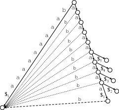
For the time being, we assume that each string is terminated with a unique symbol . Consider a subset of strings such that for each , . We then prepend the other character from the binary alphabet to each in increasing order of . For , Weiner links to the new leaf for , each labeled , are created. See Figure 4 for illustration of this step.
Then, for each , inserting a new leaf for requires an insertion of a new internal node as the parent of the new leaf. This splits the set of in-coming Weiner links into two sets: one is a singleton consisting of the Winer link from node , and the other consists of the Weiner links from the shallower nodes. Each of these split operations can be done by a simple deletion operation on the corresponding AVL tree, using time each. See Figure 5 for illustration.
Observe also that the same analysis holds even if we remove the terminal symbol from each string (in this case, there is a non-branching internal node for each and we start the climbing up process from this internal node).
The total length of these strings is approximately . We can arbitrarily choose the last string of length approximately so that it does not affect the above split operations (e.g., a unary string or would suffice).
Thus, there exists an instance over a binary alphabet for which the node split operations require total time. ∎
Since , the term is always dominated by the term. It is left open whether there exists a set of strings with character additions, each of which requires splitting a set that involves in-coming Weiner links. If such an instance exists, then our algorithm must take time in the worst case.
5 Conclusions and future work
In this paper we considered the problem of maintaining the suffix tree and the DAWG indexing structures for a collection of multiple strings that are updated in a fully-online manner, where a new character can be added to the left end or the right end of any string in the collection, respectively. Our contributions are simple pointer-machine algorithms that work in time and space, where is the total length of the strings, is the alphabet size, and is the maximum number of in-coming Weiner links of a node in the suffix tree. The key idea was to reduce the sub-problem of re-directing in-coming Weiner links to the ordered split-insert-find problem, which we solved in time by AVL trees. We also discussed the cases where our -time solution is optimal.
A major open question regarding the proposed algorithms is whether there exists an instance over a small alphabet which contains positions each of which requires time for the split operation, or requires insertions each taking time. If such instances exist, then the running time of our algorithms may be worse than the optimal for small . So far, we have only found an instance with that takes sub-linear total time for split operations.
Acknowledgements
This work is supported by JST PRESTO Grant Number JPMJPR1922.
References
- [1] G. Adelson-Velsky and E. Landis. An algorithm for the organization of information. Proceedings of the USSR Academy of Sciences (in Russian), 146:263–266, 1962. English translation by Myron J. Ricci in Soviet Mathematics - Doklady, 3:1259–1263, 1962.
- [2] A. Blumer, J. Blumer, D. Haussler, A. Ehrenfeucht, M. T. Chen, and J. Seiferas. The smallest automaton recognizing the subwords of a text. Theoretical Computer Science, 40:31–55, 1985.
- [3] A. Blumer, J. Blumer, D. Haussler, R. Mcconnell, and A. Ehrenfeucht. Complete inverted files for efficient text retrieval and analysis. J. ACM, 34(3):578–595, 1987.
- [4] M. Crochemore and W. Rytter. Text Algorithms. Oxford University Press, 1994.
- [5] H. H. Do and W. Sung. Compressed directed acyclic word graph with application in local alignment. Algorithmica, 67(2):125–141, 2013.
- [6] M. Farach-Colton, P. Ferragina, and S. Muthukrishnan. On the sorting-complexity of suffix tree construction. J. ACM, 47(6):987–1011, 2000.
- [7] Y. Fujishige, Y. Tsujimaru, S. Inenaga, H. Bannai, and M. Takeda. Computing DAWGs and minimal absent words in linear time for integer alphabets. In MFCS 2016, pages 38:1–38:14, 2016.
- [8] H. N. Gabow and R. E. Tarjan. A linear-time algorithm for a special case of disjoint set union. Journal of Computer and System Sciences, 30:209–221, 1985.
- [9] D. Gusfield and J. Stoye. Linear time algorithms for finding and representing all the tandem repeats in a string. J. Comput. Syst. Sci., 69(4):525–546, 2004.
- [10] D. Hendrian, S. Inenaga, R. Yoshinaka, and A. Shinohara. Efficient dynamic dictionary matching with DAWGs and AC-automata. Theor. Comput. Sci., 792:161–172, 2019.
- [11] H. Imai and T. Asano. Dynamic orthogonal segment intersection search. J. Algorithms, 8(1):1–18, 1987.
- [12] D. Knuth. The Art Of Computer Programming, vol. 3: Sorting And Searching, Second Edition. Addison-Wesley, 1998.
- [13] G. Kucherov and M. Rusinowitch. Matching a set of strings with variable length don’t cares. Theor. Comput. Sci., 178(1-2):129–154, 1997.
- [14] D. D. Sleator and R. E. Tarjan. A data structure for dynamic trees. J. Comput. Syst. Sci., 26(3):362–391, 1983.
- [15] D. D. Sleator and R. E. Tarjan. Self-adjusting binary search trees. J. ACM, 32(3):652–686, 1985.
- [16] T. Takagi, S. Inenaga, H. Arimura, D. Breslauer, and D. Hendrian. Fully-online suffix tree and directed acyclic word graph construction for multiple texts. Algorithmica, 82(5):1346–1377, 2020.
- [17] Y. Tanimura, Y. Fujishige, T. I, S. Inenaga, H. Bannai, and M. Takeda. A faster algorithm for computing maximal -gapped repeats in a string. In SPIRE 2015, pages 124–136, 2015.
- [18] R. E. Tarjan. A class of algorithms which require nonlinear time to maintain disjoint sets. J. Comput. Syst. Sci., 18(2):110–127, 1979.
- [19] P. Weiner. Linear pattern-matching algorithms. In Proc. of 14th IEEE Ann. Symp. on Switching and Automata Theory, pages 1–11, 1973.
- [20] J. Westbrook. Fast incremental planarity testing. In ICALP 1992, pages 342–353, 1992.
- [21] J. Yamamoto, T. I, H. Bannai, S. Inenaga, and M. Takeda. Faster compact on-line Lempel-Ziv factorization. In STACS 2014, pages 675–686, 2014.