Point Cloud Structural Similarity-based
Underwater Sonar Loop Detection
Abstract
In order to enable autonomous navigation in underwater environments, a map needs to be created in advance using a Simultaneous Localization and Mapping (SLAM) algorithm that utilizes sensors like a sonar. At this time, loop closure is employed to reduce the pose error accumulated during the SLAM process. In the case of loop detection using a sonar, some previous studies have used a method of projecting the 3D point cloud into 2D, then extracting keypoints and matching them. However, during the 2D projection process, data loss occurs due to image resolution, and in monotonous underwater environments such as rivers or lakes, it is difficult to extract keypoints. Additionally, methods that use neural networks or are based on Bag of Words (BoW) have the disadvantage of requiring additional preprocessing tasks, such as training the model in advance or pre-creating a vocabulary. To address these issues, in this paper, we utilize the point cloud obtained from sonar data without any projection to prevent performance degradation due to data loss. Additionally, by calculating the point-wise structural feature map of the point cloud using mathematical formulas and comparing the similarity between point clouds, we eliminate the need for keypoint extraction and ensure that the algorithm can operate in new environments without additional learning or tasks. To evaluate the method, we validated the performance of the proposed algorithm using the Antarctica dataset obtained from deep underwater and the Seaward dataset collected from rivers and lakes. Experimental results show that our proposed method achieves the best loop detection performance in both datasets. Our code is available at https://github.com/donghwijung/point_cloud_structural_similarity_based_underwater_sonar_loop_detection.
I Introduction
In order for marine vehicles such as submarines or ships to autonomously navigate, mapping of the underwater environment is necessary. For underwater mapping, SLAM using sonar is widely used[1, 2, 3]. Similarly to SLAM using LiDAR or cameras, pose errors accumulate in sonar SLAM as the path length increases. To reduce these accumulated errors, loop closure is used in SLAM[4, 5, 6, 7, 8]. Loop closure applies a loop constraint between the nodes in the pose graph when the current location is determined to be the same as a previously visited location, thus optimizing the entire pose graph and removing the accumulated pose errors between the two nodes. By eliminating pose errors in this way, it is possible to create an accurate 3D bathymetric map of the underwater environment.
As shown in Table I, various loop detection methods using sonar have been proposed [5, 6, 7, 8]. First, methods such as sonar context[5] find loops based on the similarity between images. However, image-based comparisons depend on the Field of View (FoV) of the sensor data used to capture the images. For example, even if it is a loop, it is difficult to identify the same location when approached from different directions, especially when using sensors like the Multibeam Echosounder (MBES) that do not have a 360-degree FoV. Moreover, in deep-sea environments with minimal horizontal features, the forward-mounted MBES may fail to capture features, making sonar context less effective. Among the studies mentioned, there are methods that project point clouds into 2D images and then use them, such as [6], and methods that directly use point clouds as input, such as [7, 8]. When loops are detected after projecting point clouds into 2D images, as in [6], information loss occurs due to the overlap of points during the projection process[9]. In contrast, methods that directly use point clouds as input, such as [7, 8], do not suffer from such information loss. However, these methods have the disadvantage of requiring separate preprocessing tasks, such as training a neural network model according to the environment or creating a new vocabulary, for the loop detection task.
| Input Data | Method | Description | Bathymetry | w/o 2D Projection | w/o Preprocessing | |
| Sonar context [5] | Image | Rule-based | Polar images matching | ✓ | ||
| Hammond et al. [6] | Point cloud | Rule-based | Image key points matching | ✓ | ✓ | |
| Tan et al. [7] | Point cloud | Learning-based | Point cloud key points matching | ✓ | ✓ | |
| Shape BoW [8] | Point cloud | Representation | Gradient features & Bag-of-Words | ✓ | ||
| This work | Point cloud | Rule-based | Point cloud structural similarity | ✓ | ✓ | ✓ |
In this paper, we detect the loop based on the point cloud structural similarity. The structured geometry of MBES data facilitates easy conversion into 3D point clouds, which we use as measurements. In addition, the viewing direction of the MBES is set downward. This choice is motivated by the lack of features in the horizontal direction in deep-sea environments [10]. Even in marine environments with few horizontal features, the downward direction can capture relatively more features. The point cloud conversion of a single sonar data sequence represents a linear distribution along a single channel. Therefore, when approaching the same location from different directions, there is minimal overlap between point clouds, making it difficult to identify loops. To address this, we accumulate consecutive point clouds before and after the sequence of interest for loop detection. In this process, square cropping was applied to extract points within a certain distance from the ego-vehicle in the directions, and these were used as input point cloud. The reason for applying this square cropping is that in the case of cylindrical cropping, as applied in [7], the circular shape has less overlap between loop pair point clouds compared to the square shape, leading to relatively poorer results when comparing similarity. This outcome is demonstrated through experiments in this paper.
To overcome the drawbacks of learning-based and representation methods that rely on training data, we calculate the similarity between feature maps generated by transforming the point cloud’s structural features, calculated considering the relationship with each point’s neighborhood, as proposed in PointSSIM [11]. We use these feature maps to calculate similarity between point clouds, with the goal of recognizing loops even when the vehicle approaches the same location from different directions. Typically, structural features of point clouds, such as geometry and normals, change with the rotation of the point cloud, making it difficult to compare the similarity of point clouds taken from the same location but rotated differently. However, feature maps calculated considering the relationship with each point’s neighborhood have rotation-invariant values, allowing for loop detection even when approaching the same location from different directions. Finally, after calculating the similarity using these feature maps, we identify loop pairs with high similarity exceeding a certain threshold.
Our proposed method does not require a model or vocabulary, making it easily applicable to various environments such as deep seas, rivers, and lakes, compared to existing methods. In addition, by using a point-wise structural feature map to calculate the similarity of the point cloud, it has the advantage of operating robustly even in environments with simple slopes on the surface, compared to traditional keypoint-based methods.
The contributions of our paper are as follows:
-
•
We propose a method that, by comparing the structural characteristics of point clouds, can be directly applied to new environments without requiring additional training or vocabulary creation, unlike previous methods.
-
•
We propose a method that robustly identifies loop pairs using the point-wise structural similarity of point clouds without 2D image projection, enabling the detection of loop pairs even in monotonous seafloor environments.
II Related Works
There have been previous attempts to perform loop detection in underwater environments using sonar [6, 7, 8]. Initially, Hammond et al.[6] projected 3D point clouds into 2D and then matched features typically used in 2D images, such as SIFT [12], to find loops. However, when there were significant changes in depth due to uneven seabeds, a large number of keypoints were extracted because of the substantial changes in depth between image pixels. As mentioned earlier, this method suffered from information loss due to resolution limitations during the projection of 3D point clouds into 2D. Additionally, in environments with relatively flat bottoms, such as rivers or lakes, few keypoints could be found after image projection, presenting another disadvantage.
On the other hand, Tan et al.[7] used the point cloud directly as input to the algorithm without any projection. The authors generated the input point cloud by transforming multiple consecutive point clouds over a certain period using dead reckoning and then accumulating those point clouds into a single point cloud. They also applied cylindrical cropping to ensure that the point cloud remained the same regardless of the vehicle’s orientation at the same location. In this case, the cylindrically cropped point cloud allowed for uniform overlap regardless of the ego-vehicle’s direction, making loop detection easier. In the study, the key points were extracted using a network and the distance between the points that matched the source and the target was calculated. The existence of a loop was then determined based on a predefined threshold. However, one drawback of cylindrical cropping was that as the distance between loops increases, the overlap area of the point clouds becomes significantly smaller, reducing accuracy in similarity calculations. Moreover, the method relied heavily on the network for the dataset, which complicated the differentiation of various parameters and required additional training for each environment.

In addition, Zhang et al.[8] proposed a modified BoW approach called Shape BoW. The research calculated the standard deviation of the depth between adjacent points and used this for BoW training to perform loop detection. After that, they converted point clouds into images before performing loop detection. Because the method did not depend on keypoint extraction, it achieves relatively higher accuracy. However, this BoW-based method is performance dependent on the vocabulary. The vocabulary was created by clustering pre-extracted descriptors and converting them into a certain number of words, which were then stored. When the environment in which the dataset was obtained changed, the distribution of the descriptors also changed, requiring the creation of a new vocabulary. Thus, applying this BoW method immediately to new environmental changes was difficult.
For these reasons, we propose a method that minimizes data loss and can be generally applied in various environments using a mathematical technique. Our method transforms the structural features of the point cloud into rotation-invariant feature maps and compares similarities between those feature maps, allowing for accurate performance across different environments. Additionally, since it does not rely on 2D projection or keypoint extraction, our experiments demonstrate superior performance compared to existing methods.
III Methods
III-A Dead Reckoning
In the case of a downward-facing MBES, the beams spread widely in the lateral direction, while they are relatively narrow in the forward and backward directions of the vehicle. Therefore, when reconstructing point clouds from data of a single sequence obtained by MBES, the resulting point cloud, when viewed vertically, resembles single-channel 2D LiDAR data with a limited FoV. In underwater autonomous navigation scenarios, when data is collected downward, there is hardly any overlap when approaching the same location from different directions due to the single-channel nature. Thus, this single-channel point cloud cannot be used to find underwater terrain loops. To overcome this, we utilized IMU sensors to acquire linear acceleration, angular velocity, and magnetic field data, which were then input into an IMU filter to calculate orientation. The gyro-corrected orientation of the ego-vehicle is used to transform the local coordinate-based speed obtained from the Doppler Velocity Log (DVL) sensor into speed based on reference coordinates. Then, using velocity-time integration, the relative transformation in the reference coordinates is calculated. The process is expressed mathematically as follows:
| (1) | |||
| (2) | |||
| (3) | |||
| (4) |
where represents the local velocity, which corresponds to the velocity values measured by the DVL. is the orientation of the ego vehicle and represents the global velocity, which is the local velocity transformed into global coordinates by multiplying it by the orientation of the ego vehicle. denotes the time interval between timestep and . refers to the position of the ego vehicle in global coordinates. and respectively signify the orientation and position of the ego vehicle at the reference point in time. and respectively refer to the local orientation and position, where the local coordinate system is based on the pose of the ego vehicle at the starting point.
III-B Point Cloud Processing
For the data acquired by MBES, each beam has values for distance and angle. When these values are converted into points with coordinates, they form a point cloud that can be obtained from a single sequence [13]. The point cloud obtained from a single sequence of MBES data resembles single-channel data. In such single-channel data, there is minimal overlap when data is acquired from different directions, making loop detection difficult. Therefore, it is necessary to merge consecutive data to augment the information obtained from a specific location. During this process, dead reckoning using DVL and IMU sensors is employed to calculate transformations and accumulate consecutive point clouds. The accumulated point clouds are then cropped in a square shape around the axis centered on the current position of the vehicle, based on a predefined distance. This point cloud processing procedure is as follows:
| (5) | |||
| (6) |
where represent the positions of points in the point cloud obtained from the 3D transformation of the raw data from the MBES. denotes the point cloud composed of these points . and are the current relative rotation and translation transformations calculated in Sec. III-A. is a predefined value that corresponds to half of the time sequence to accumulate the point cloud. refers to the accumulated point cloud created by transforming the point clouds based on the current pose using and . indicates the Manhattan distance. is the reference point of , corresponding to the current pose of the vehicle. and represent the coordinates and of the respective point. is a predefined value used for square cropping . is the point cloud obtained as a result of the square cropping.

III-C Feature Maps
To calculate the similarity between point clouds, we created feature maps using the structural features of the point cloud in this paper. Initially, we utilized three types of features: geometry, normals, and curvature. Geometry is represented by the Euclidean distance between each point in the point cloud and its neighboring points. For normals, it involves the angle between the normal vectors of each point and its neighbors. The reason for not directly using the position information of the points and their normal vectors, which are commonly used for geometry and normal features, is that these values are rotation-variant. Since our research also addresses loop detection when passing the same place with different orientations, we use rotation-invariant geometry and normal features. For curvature, it represents the mean curvature for each point. The calculations for the feature maps and the curvature are referenced from [11] and [14], respectively. The process of creating the quantity, which is the prior stage of the feature map from a square-shaped cropped point cloud is as follows:
| (7) | |||
| (8) | |||
| (9) | |||
| (10) | |||
| (11) |
where , , and represent the geometry, normal, and curvature quantities at point , respectively. Additionally, , , and are the sets of , , and in Eq. (7). Furthermore, , , and denote the Euclidean distance, the cardinality of the set, and the size of the vector, respectively. denotes the -th nearest neighbor point of . refers to the number of the nearest neighbors. in Eq. (9) represents the normal vector calculated at by plane fitting and indicates the normal vector at . In Eq. (11), , , , , and represent the coefficients of the quadric surface , fitted using and the nearest-neighbor points. This quadric surface fitting is based on the method described in [14].
As shown in Fig. 2, for these calculated quantities, we create a feature map by calculating the mean and variance of the values of each quantity for the neighborhood point by point. By using representative values such as mean and variance, we reduce the dimension of the data used to calculate point cloud similarity, thereby shortening the computation time.
| (12) | |||
| (13) | |||
| (14) | |||
| (15) | |||
| (16) |
where the subscripts and under denote the methods used to calculate the feature maps, corresponding to mean and variance, respectively. refers to any element of the entire set of feature maps possessed by a single point cloud. indicates the set of feature maps . In addition, denotes the feature map of point . and represent the mean and variance of the feature at point , respectively, and correspond to elements of and .


III-D Loop Detection
We calculate similarity by comparing the point cloud feature map, computed in Sec. III-C, with the feature maps of previously stored point clouds. The sum of similarities obtained in this manner is identified and, if it exceeds a predefined threshold, it is considered a loop. This process can be mathematically expressed as follows:
| (17) | |||
| (18) | |||
| (19) | |||
| (20) |
where is the structural similarity between the first two elements calculated based on the third element. Moreover, indicates the absolute value. is a constant that is used to prevent the denominator in from being zero. indicates similarity between two point clouds corresponding to the average of similarities of the feature maps. represents the threshold for each feature map used to determine whether it constitutes a loop. Lastly, is the indicator function to determine whether two sequences are a loop pair or not.
IV Experiments
IV-A Purposes and Details
The two research questions we aim to verify in this paper are as follows: 1) Does the proposed method demonstrate good loop detection performance in various environments without preprocessing tasks such as model training or creating a vocabulary? 2) Does the method perform well even in monotonous underwater environments by utilizing the point-wise information of the 3D point cloud? To answer the first research question, we compared the proposed method’s loop detection performance against the method by Tan et al.[7], which trains a neural network model for each dataset, and Shape BoW [8], which generates a vocabulary for each dataset. To address the second question, we verified whether the proposed method can successfully detect loops even in environments where few appropriate keypoints are detected for loop detection. Additionally, for comparative validation, we compared the loop detection performance on the same datasets with a keypoint-based method, such as Hammond et al. [6].
In this experiment, we evaluated the performance of the proposed algorithm using the Antarctica dataset, obtained using the Hugin 3000 AUV [7], and the Seaward dataset, acquired from banks via boats [15]. To compare the performance of the proposed method, we used studies that employed sonar sensors for bathymetric purposes [6, 7, 8] as baselines. Since the code for [6, 8] was not publicly available, we implemented the algorithms based on the descriptions in the respective papers, except for [7]. Moreover, to test the method by Tan et al., we trained a neural network model using each dataset. Similarly, we created a vocabulary for each dataset and validated the performance of Shape BoW. For the Antarctica dataset, where the depth was greater and the lateral spread was wider, the distance parameter was set to based on the criteria in [7].


In contrast, for the Seaward dataset, due to its shallow depth, the lateral spread of the vehicle-based point cloud was narrower, thus was set to for square cropping, as in Eq. (6). The determination of positive and negative pairs between two sequences was based on the Euclidean distance of the ego-vehicle pose. If the distance was smaller than , the pair was considered a positive pair, while distances greater than were considered negative pairs. For the Seaward dataset, experiments were conducted across four different environments: Wiggles Bank, North River, Dutch Island, and Beach Pond.
IV-B Evaluation
IV-B1 Antarctica
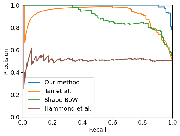
The experimental results in the Antarctica dataset are shown in Fig. 4(a). When comparing the results based on Average Precision (AP), which represents the area under the Precision-Recall curve, the AP of our proposed method and Tan et al. are the highest, confirming that both methods achieve good loop detection performance. Shape BoW shows moderate prediction performance, while the method by Hammond et al. demonstrates the lowest performance. From this, we can answer the first research question: unlike the methods by Tan et al. and Shape BoW, which require separate model training or vocabulary creation, our proposed method achieve the best loop detection performance without any additional preprocessing. Furthermore, since the method by Hammond et al., which is based on keypoint-based loop detection, does not perform well, the good performance of our proposed method indicates that it works well even in environments where it is difficult to extract appropriate keypoints for loop detection. This also allow us to answer the second research question.
IV-B2 Seaward
The performance of each method on the second Seaward dataset is shown in Fig. 4(b), 4(c), 4(d), and 4(e). While there are slight differences in the performance of each algorithm across the four datasets, overall, the proposed method demonstrated the best performance. Therefore, we verify that the proposed method works well in new environments without requiring additional preprocessing, answering the first research question. Tan et al. and Shape BoW show similar levels of performance, while Hammond et al., as in the previous case with the Antarctica dataset, shows the lowest loop detection performance. The reason for the relatively poor performance of Tan et al. compared to the Antarctica dataset is attributed to the differences between the Antarctica and Seaward datasets. In the case of the Seaward dataset, data was collected in relatively shallow and flat environments, such as lakes and rivers. As a result, keypoint-based loop detection methods like Tan et al. and Hammond et al. perform poorly on the Seaward dataset.
IV-B3 Ablation study
We conducted an ablation study on the cropping of input data from point clouds. First, as proposed in Sec. III-B, we cropped the accumulated point cloud along the ego-vehicle’s path into a square shape. This method, applied in [6, 8], which convert point clouds into grid images. Furthermore, referencing [7], we performed cylindrical cropping to compare the performance of loop detection. Cylindrical cropping has the advantage that, when passing through a similar location, the point clouds overlap uniformly regardless of the ego-vehicle’s orientation. After cropping the point clouds using these two different methods, we compared the results of loop detection. As shown in Fig. 4(f), it was confirmed that square cropping demonstrated higher loop detection performance than cylindrical cropping. This result can be attributed to the fact that, square cropping includes regions near the corners outside of the circular area, which leads to a larger overlap when the point clouds are misaligned.
V Conclusion
In this paper, we proposed a loop detection algorithm based on the comparison of structural similarity in point clouds obtained through MBES in underwater scenarios. Unlike learning-based methods that require model training or BoW-based methods that require vocabulary creation, our proposed method can accurately detect loops in various environments, such as deep seas, rivers, and lakes, without any additional preprocessing. Moreover, by comparing sequences using the point-wise characteristics of the 3D point cloud without 2D projection, the method could accurately detect loops even in simple environments where it was difficult to extract keypoints from the seafloor. To validate the performance of the proposed method, experiments were conducted using data collected from diverse environments, including the Antarctica and Seaward datasets. The results confirmed that the proposed algorithm is a robust MBES-based underwater loop detection method suitable for various marine and underwater environments.
Acknowledgments
This research was supported by Korea Institute for Advancement of Technology(KIAT) grant funded by the Korea Government (MOTIE) (P0017304, Human Resource Development Program for Industrial Innovation) and by the Korean Ministry of Land, Infrastructure and Transport (MOLIT) through the Smart City Innovative Talent Education Program. Research facilities were provided by the Institute of Engineering Research at Seoul National University.
References
- [1] C. Cheng, C. Wang, D. Yang, W. Liu, and F. Zhang, “Underwater localization and mapping based on multi-beam forward looking sonar,” Frontiers in Neurorobotics, vol. 15, p. 801956, 2022.
- [2] Q. Zhang and J. Kim, “Ttt slam: A feature-based bathymetric slam framework,” Ocean Engineering, vol. 294, p. 116777, 2024.
- [3] J. Zhang, Y. Xie, L. Ling, and J. Folkesson, “A fully-automatic side-scan sonar simultaneous localization and mapping framework,” IET Radar, Sonar & Navigation, vol. 18, no. 5, pp. 674–683, 2024.
- [4] M. M. Santos, G. B. Zaffari, P. O. Ribeiro, P. L. Drews-Jr, and S. S. Botelho, “Underwater place recognition using forward-looking sonar images: A topological approach,” Journal of Field Robotics, vol. 36, no. 2, pp. 355–369, 2019.
- [5] H. Kim, G. Kang, S. Jeong, S. Ma, and Y. Cho, “Robust imaging sonar-based place recognition and localization in underwater environments,” arXiv preprint arXiv:2305.14773, 2023.
- [6] M. Hammond, A. Clark, A. Mahajan, S. Sharma, and S. Rock, “Automated point cloud correspondence detection for underwater mapping using auvs,” in OCEANS 2015-MTS/IEEE Washington. IEEE, 2015, pp. 1–7.
- [7] J. Tan, I. Torroba, Y. Xie, and J. Folkesson, “Data-driven loop closure detection in bathymetric point clouds for underwater slam,” in 2023 IEEE International Conference on Robotics and Automation (ICRA). IEEE, 2023, pp. 3131–3137.
- [8] Q. Zhang and J. Kim, “Shape bow: Generalized bag of words for appearance-based loop closure detection in bathymetric slam,” IEEE Robotics and Automation Letters, 2024.
- [9] Q. Yang, H. Chen, Z. Ma, Y. Xu, R. Tang, and J. Sun, “Predicting the perceptual quality of point cloud: A 3d-to-2d projection-based exploration,” IEEE Transactions on Multimedia, vol. 23, pp. 3877–3891, 2020.
- [10] K. J. Lohmann and C. M. Lohmann, “Orientation and open-sea navigation in sea turtles,” Journal of Experimental Biology, vol. 199, no. 1, pp. 73–81, 1996.
- [11] E. Alexiou and T. Ebrahimi, “Towards a point cloud structural similarity metric,” in 2020 IEEE International Conference on Multimedia & Expo Workshops (ICMEW). IEEE, 2020, pp. 1–6.
- [12] D. G. Lowe, “Distinctive image features from scale-invariant keypoints,” International journal of computer vision, vol. 60, pp. 91–110, 2004.
- [13] H. Cho, B. Kim, and S.-C. Yu, “Auv-based underwater 3-d point cloud generation using acoustic lens-based multibeam sonar,” IEEE Journal of Oceanic Engineering, vol. 43, no. 4, pp. 856–872, 2017.
- [14] G. Meynet, Y. Nehmé, J. Digne, and G. Lavoué, “Pcqm: A full-reference quality metric for colored 3d point clouds,” in 2020 Twelfth International Conference on Quality of Multimedia Experience (QoMEX). IEEE, 2020, pp. 1–6.
- [15] K. Krasnosky, C. Roman, and D. Casagrande, “A bathymetric mapping and slam dataset with high-precision ground truth for marine robotics,” The International Journal of Robotics Research, vol. 41, no. 1, pp. 12–19, 2022.