Point Cloud Resampling via Hypergraph Signal Processing
Abstract
Three-dimensional (3D) point clouds are important data representations in visualization applications. The rapidly growing utility and popularity of point cloud processing strongly motivate a plethora of research activities on large-scale point cloud processing and feature extraction. In this work, we investigate point cloud resampling based on hypergraph signal processing (HGSP). We develop a novel method to extract sharp object features and reduce the data size of point cloud representation. By directly estimating hypergraph spectrum based on hypergraph stationary processing, we design a spectral kernel-based filter to capture high-dimensional interactions among point signal nodes and to better preserve object surface outlines. Experimental results validate the effectiveness of hypergraph in representing point clouds, and demonstrate the robustness of the proposed algorithm under noise.
Index Terms:
Compression, hypergraph signal processing, point cloud resampling, virtual reality.I Introduction
The widespread deployment of networked sensors and cameras is a critical element of IoT. In visualization applications, 3D point clouds provide efficient data representation of external surfaces for objects and their surroundings. Point clouds have found wide applications in recent years, including surface reconstruction [1], rendering [2] and feature extraction [3]. High data volume of point cloud representation poses challenges to data transport and storage. One important point cloud processing task involves resampling for reducing the data size in a point cloud while preserving vital 3D structural features. Point cloud resampling serves important practical applications such as segmentation, object classification, and data compression.
The literature contains a variety of works on point cloud resampling. A centroidal Voronoi tessellation based method in [4] can progressively generate high-quality resampling results with isotropic or anisotropic distributions from a given point cloud. The 3D downsampling technique based on a growing neural gas network developed in [5] deals with data outliers and can represent 3D spaces by an induced Delaunay triangulation of the input space. Importantly, graph-based resampling has exhibited attractive capability to capture some underlying structures of point clouds [6, 7]. For example, the work [8] focused on computationally efficient resampling and proposed several graph-based filters to capture the distribution of point data. Another graph-based example is a graph-based contour-enhanced resampling method presented in [9]. We also note a different, feature-based, approach to point cloud resampling based on edge detection and feature extraction. In [10], the authors presented a sharp feature detector using Gaussian map clustering on local neighborhoods. Bazazian and co-authors [11] extended this principle by leveraging principal component analysis (PCA) to develop a new agglomerative clustering method. This work establishes speed and accuracy improvement by analyzing the eigenvalues of covariance matrix defined by nearest neighbors.
Despite these and other successes, graph-based and feature-based resampling methods still need to overcome some limitations. For graph-based methods, each graph edge can only model pairwise relationships even though multilateral interactions of point data represent highly informative characteristics of 3D objects. For example, bilateral connections only partially represent multilateral relationship among multiple points on the same surface. Another open issue relates to the efficient construction of a graph for an arbitrary point cloud. Among feature-based methods, how to select adequate features and filter parameters remains a practical design challenge. The development of a general model with robust parameter selection remains an open problem.
There have been some reported successes at applying hypergraphs to model and characterize the multilateral interactions among multimedia data points [12]. Hypergraph consists of nodes and hyperedges. Since each hyperedge can include more than two nodes, hypergraph provides a more general tool in point cloud processing to model multilateral point relationships on object surfaces. Furthermore, as a generalization of graph signal processing (GSP) [13], hypergraph signal processing (HGSP) [14, 15] has enjoyed additional notable successes in processing point clouds for segmentation, sampling, and denoising [16, 17].
In this paper, we propose a novel 3D point cloud resampling method using kernel filtering based on hypergraph signal processing. Leveraging hypergraph stationary process, we first estimate hypergraph kernel basis for a point cloud. We further define a local smoothness with respect to high-pass filtering in spectrum domain for resampling. In order to test the model preserving property on complex models, we develop a simple method for point cloud recovery based on alpha complex and Poisson sampling. Our experimental results demonstrate the compression efficiency and robustness of our proposed point-cloud resampling method.
II Background
II-A Point Cloud
A point cloud is a collection of point coordinates in 3D space. In point clouds, each point consists of three coordinates and may contain additional features, such as colors and normals [18]. In this work, we focus on the coordinates of these points when resampling point clouds. These point coordinates are represented by the location matrix , where is the number of points in the point cloud and is the 3D coordinates of the -th point.
II-B Hypergraph Signal Processing
Hypergraph signal processing (HGSP) is a framework based on the tensor representation of hypergraphs to capture high-order signal interactions [14]. In this framework, an th-order -dimensional representing tensor represents a hypergraph with vertices, where each hyperedge is capable of connecting at most nodes. Weights of hyperedges connecting fewer than nodes are normalized according to combinations and permutations [19].
Orthogonal CANDECOMP/PARAFAC (CP) method enables approximate decomposition of a representing tensor into , where denotes tensor outer product, are orthonormal basis to represent spectrum components, and is corresponding frequency coefficient. Spectrum components {} form the full hypergraph spectral space. Other HGSP concepts, such as filtering, hypergraph Fourier transform, and sampling theory can be defined [14].
III HGSP Point Cloud Resampling
In this section, we introduce our kernel-based resampling method. Generally, our proposed method consists of three main steps: i) hypergraph spectrum construction, ii) Fourier transform, iii) high-pass filtering and resampling.
We first estimate hypergraph spectrum based on hypergraph stationary process. Shown in [17], a stochastic signal is weak-sense stationary iff it has zero-mean and its covariance matrix has the same eigenvectors as the hypergraph spectrum basis, i.e., and where is the hypergraph spectrum. We can estimate the hypergraph spectrum from the covariance matrix of three coordinates by assuming the signals to be stationary. Here, we use the same spectrum estimation strategy as [17], and consider the adjacency tensor as a third-order tensor which is the minimal number of nodes to form a surface.
We define a 3D cube as the kernel to define a local signal . For simplicity, we use a cube as the kernel in this paper, although larger kernel can facilitate flexibility in filter design at the cost of complexity. Let be the center distance between two nearby voxels in the kernel. A proper selection of should allow to capture local geometric information. If is too small, only a few neighbors of the -th point are included in the , leading to noise-sensitivity. If is too large, many neighbors are included in each voxel, which may lead to blurred local geometric information. A typical choice of is the intrinsic resolution of a point cloud. We place the kernel towards the bounding box of the point cloud in our experiment.
Let be the coordinates of the total voxel centers in the kernel. For our selected kernel, . We then normalize the coordinates to define a zero mean signal . By calculating eigenvectors for , we can estimate hypergraph spectrum .
Next, for -th point in the point cloud, its corresponding local signal is defined according to the number of points in the voxel of kernel centered at point . By focusing on 3rd-order tensors and signal energies in spectrum domain, we can utilize hypergraph spectrum to calculate a simplified-form of hypergraph Fourier transform as
| (1) |
For edge-preserving purpose, we would like to separate high frequency coefficients from low frequency coefficients in spectrum domain. Since the spectrum bases corresponding to smaller represent higher frequency components[14], we can sort eigenvalues of as with corresponding eigenvectors {}. We can then devise a threshold for dividing high frequency components and low frequency components based on a sharp change between two adjacent eigenvalues.
Given a threshold selection of , we could further define a local smoothness to select resampled points:
| (2) |
which is the fraction of high frequency energy.
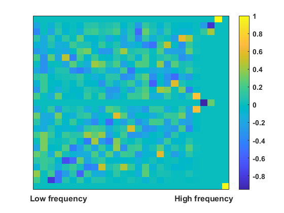
Finally, we resample the point cloud by selecting points with smaller , which corresponds to points containing larger amount of high frequency in the hypergraph. We summarize our algorithm as Algorithm 1. Since the resampled point clouds tend to favor high-frequency points, they often contain sharper features and are less smooth. Although the higher frequency basis vectors do not necessarily display a clear regular pattern, as shown in Fig. 2, they have larger total variation over the (hyper)graph, which are corresponding to sharper features. Interested readers could refer to [14, 13, 17] for a comprehensive discussion on the high frequency features in hypergraphs.
For an unorganized point cloud, the computational complexity of our method amounts to , whereas for an organized point cloud, the complexity order is .
| Combination of cubes | ||||||
|---|---|---|---|---|---|---|
| Kernel Filtering | Fast Resampling | |||||
| Noise Level | Precision | Recall | F1-Score | Precision | Recall | F1-Score |
| No noise | 0.3545 | 0.9332 | 0.5125 | 0.3827 | 1 | 0.5522 |
| 20% | 0.2556 | 0.6689 | 0.3690 | 0.2326 | 0.6086 | 0.3357 |
| 40% | 0.1052 | 0.2745 | 0.1518 | 0.0995 | 0.2600 | 0.1436 |
| Cylinder | |||||
|---|---|---|---|---|---|
| Kernel Filtering | Fast Resampling | ||||
| Precision | Recall | F1-Score | Precision | Recall | F1-Score |
| 0.2212 | 0.9298 | 0.3524 | 0.2523 | 1 | 0.3981 |
| 0.1667 | 0.6834 | 0.2647 | 0.1497 | 0.5912 | 0.2359 |
| 0.0894 | 0.3566 | 0.1412 | 0.0064 | 0.2515 | 0.1003 |
| Pyramid | ||||||
| Kernel Filtering | Fast Resampling | |||||
| Noise Level | Precision | Recall | F1-Score | Precision | Recall | F1-Score |
| No noise | 0.4567 | 0.6860 | 0.5097 | 0.6750 | 0.9034 | 0.7168 |
| 20% | 0.4191 | 0.5871 | 0.4538 | 0.4300 | 0.5696 | 0.4537 |
| 40% | 0.3017 | 0.4024 | 0.3205 | 0.2345 | 0.2874 | 0.2395 |
IV Experimental results
We now describe our experiment setup and present test results of the proposed resampling algorithm.
IV-A Edge Preserving on Simple Synthetic Point Clouds
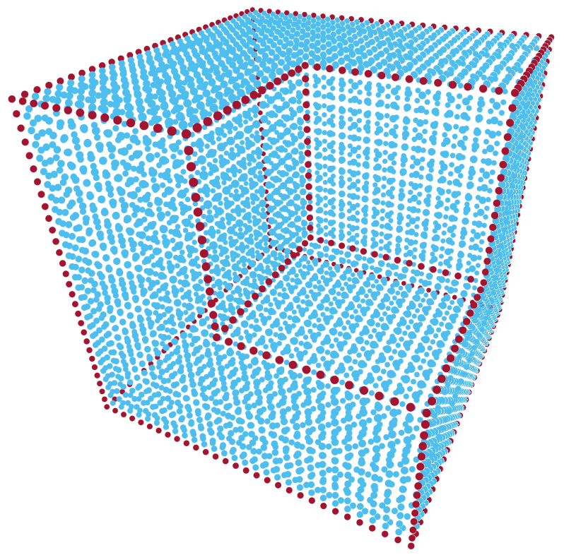
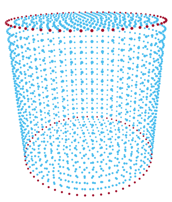
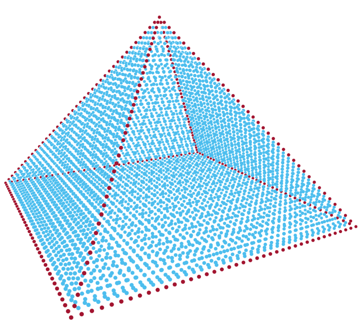
As we mentioned in Section III, one important resampling objective is to preserve sharp features in a point cloud such as edges and corners. Here, we study the edge preserving capability of our proposed algorithms by testing over several simple synthetic point clouds. The benefit for selecting synthetic point clouds is the ability to take advantage of known ground truth regarding edges and our ability to label them. We generate these synthetic point clouds by uniformly sampling external surface of models constructed from cylinders, pyramids, and combinations of cubes of various sizes. Examples of synthetic point clouds are shown in Fig. 1, where the points on edges are marked with red and the rest points are in blue.
To measure the accuracy of the edge preserving features, we use the score defined as:
| (3) |
in which precision is the proportion of points correctly preserved by the resampling algorithm whereas the recall rate is the ratio of correctly preserved edge points to all ground truth edge points.
We compare our method with a graph-based fast resampling method given in [8]. We set resampling ratio to for all point clouds. More results on different sampling ratios are in Section IV-C. The parameters of fast resampling method are set to typical values according to [8]. In order to study robustness, we include random Gaussian noise of and to the coordinates of point cloud. The noise effects on the results are shown in Table I. The test results show that our hypergraph kernel-based filtering method achieves better performance in preserving edges in noisy data when compared against GSP-based method. Since the realistic point clouds always contain noise, our proposed method is more practical in real applications.
IV-B Edge Detection on Complex Real Point Cloud
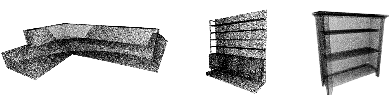
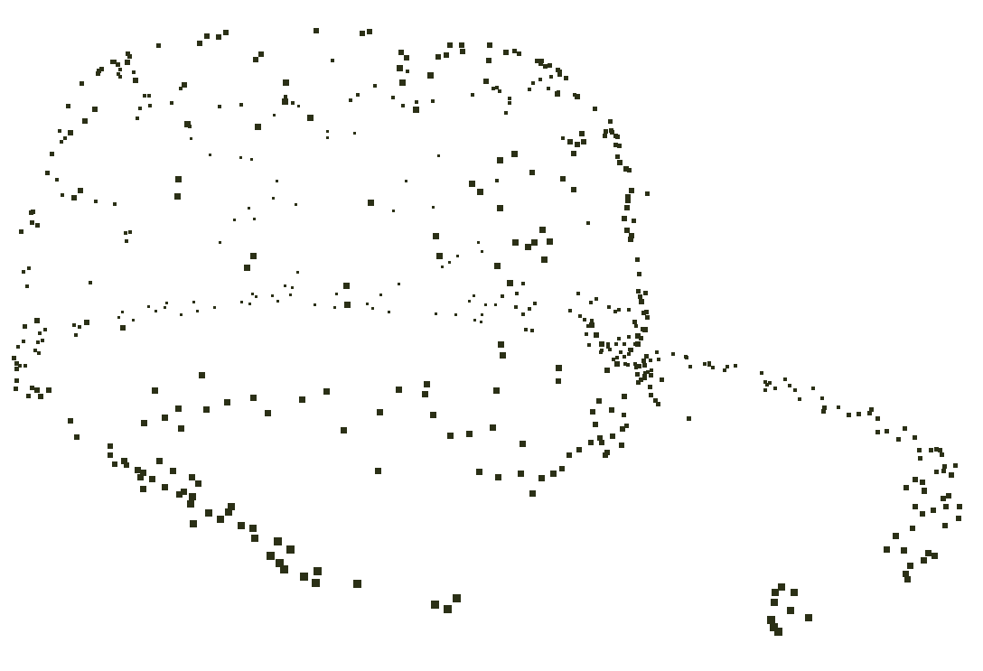
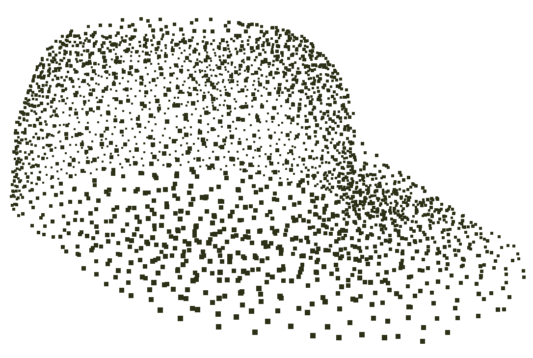
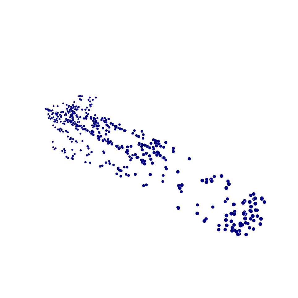
To test our proposed algorithm in a more general setting, we also implement edge-detection based on our resampled data in more complex practical point clouds. For these datasets, there are no known ground truth edges. Therefore, we shall present the matching point clouds in Fig. 3, where the top row contains the 3 original point clouds and the bottom row shows the resampled point clouds. Visual inspection shows that our resampling method easily captures contours of the objects.
| Categories | Kernel Filtering | Fast Resampling | Eigenvalues Analysis | PCA and Clustering |
|---|---|---|---|---|
| Cap | 0.0101 | 0.0102 | 0.0087 | 0.0115 |
| Chair | 0.0113 | 0.0118 | 0.0125 | 0.0126 |
| Mug | 0.0134 | 0.0141 | 0.0150 | 0.0147 |
| Rocket | 0.0069 | 0.0070 | 0.0070 | 0.0073 |
| Skateboard | 0.0080 | 0.0079 | 0.0082 | 0.0083 |
IV-C Point Cloud Recovery from Resampled Point Clouds
To study the model preservation of our proposed method, we recover original point clouds after resampling and evaluate the difference between original and the recovered point clouds.
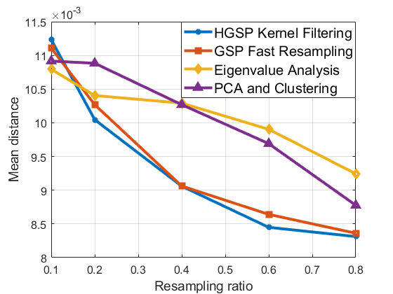
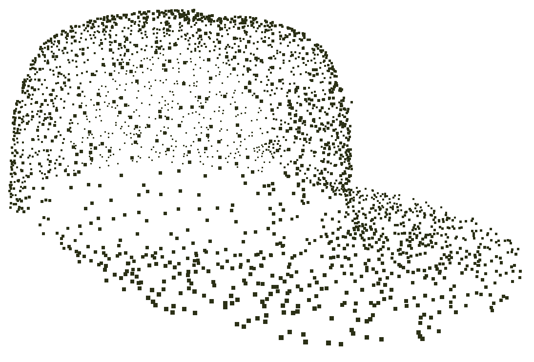
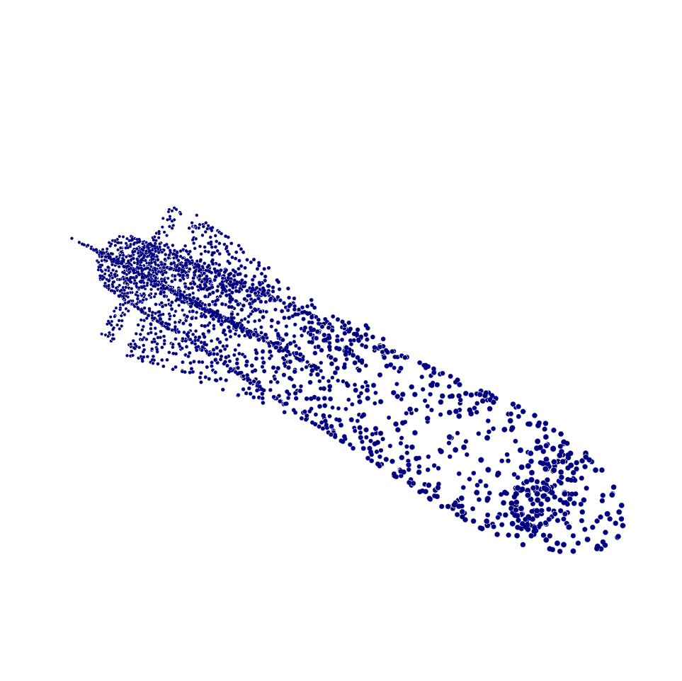
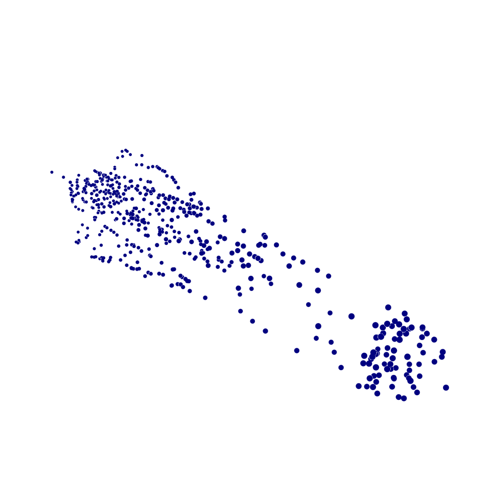
Recovery Method: The point cloud recovery contains two steps: 1) reconstruct the surface of object from resampled point cloud, and 2) sample on reconstructed surface to generate the recovered point cloud. Since many points in the edge preserving resampled point clouds are located in areas with high local variation, such as surface edges, the resampled point clouds is non-uniform, as shown in Fig. 5b. Therefore, most commonly used surface reconstruction methods such as Poisson reconstruction [20] may not be compatible with these point clouds. In order to reconstruct surfaces, we build alpha complex [21] of the resampled point cloud. To minimize the sensitivity to reconstruction, we reconstruct six different surface models based on different parameters for each resampled point cloud. We then apply Poisson-disk resampling to sample over the alpha complex to recover the original point cloud. Only the recovered point cloud with the smallest distance to the original point cloud is kept as output.
Distance between two point clouds: To measure the similarity between the original and recovered point clouds, we define a distance metric
| (4) |
where is the number of points in the original point cloud, and are points on the original and recovered point clouds, respectively. Although we apply different parameters in the reconstruction, errors such as phantom surfaces that do not exist in the original point cloud may still appear. Therefore, we select a threshold to three times the intrinsic resolution of the original point cloud. is the average distance among points of the original point cloud within from the closest points in the best recovered point cloud.
Visual and numerical results.
Our experiment uses models in six different categories in Shapenet [22] as the original point clouds. We compare our hypergraph kernel-based filtering method with the GSP-based method in [8]. We also compare to two edge detection methods, i.e., eigenvalues analysis and PCA clustering methods in [11]. We resample the same number of nodes for all methods under comparison.
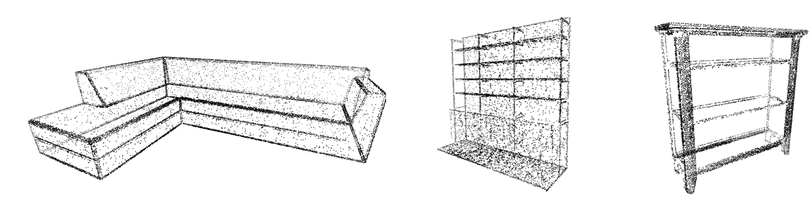
Our experiment follows the following steps: first, we use resampling and edge detection methods to calculate the resampled point clouds at different values of resampling ratio ; next, we use the proposed recovery method to generate the recovered point clouds; we then calculate the distance between the recovered point clouds and the corresponding original ones; finally, we calculate the mean distance between the best recovered point cloud and their original point cloud for each method. An example of the recovered point cloud is shown in Fig. 5c. Numerical results for are shown in Table II. Our test results show that the proposed method achieves lower mean distance than that from GSP-based resampling. When compared with edge detection methods, our proposed algorithm generates similar or smaller mean distance in most categories. Fig. 6 shows another example of point cloud resampling. The edges of the rocket tail are well preserved in our resampled results as shown in Fig. 5(b), while the GSP-based method fails to show those tails. We also examine the effect of different resampling ratio in Fig. 4 by using the same set of point clouds. Our proposed method exhibits superior performance over traditional methods in terms of mean distance for various resampling ratios. In terms of computation, we process the point cloud with 349,300 points in 50.88 seconds by using Matlab on a standard desktop (4.4 GHz Intel Core i5, 64 GB memory) without parallel processing, while the GSP-based method needs 56.82 seconds. These tests demonstrate the efficiency and efficacy of our point cloud recovery. It also shows that HGSP can model the point clouds more efficiently than regular GSP in some point cloud applications.
V Conclusion
In this work, we developed a 3D point cloud resampling method using kernel filtering based on hypergraph signal processing (HGSP). Our proposed HGSP resampling is simple and effective. Experimental results demonstrated that our HGSP method outperforms traditional graph-based methods or feature-based methods such as edge detection in terms of robustness to the noise and model preservation. This work establishes HGSP as an efficient tool to model multilateral relationship and to extract features in point cloud applications.
References
- [1] Z. C. Marton, R. B. Rusu and M. Beetz, “On fast surface reconstruction methods for large and noisy point clouds,” 2009 IEEE International Conference on Robotics and Automation, Kobe, Japan, May 2009, pp. 3218-3223.
- [2] R. Schnabel, S. Möser and R. Klein, “A Parallelly Decodeable Compression Scheme for Efficient Point-Cloud Rendering,” in SPBG, Prague, Czech Republic, Sep. 2007, pp. 119-128.
- [3] S. Gumhold, X. Wang and R. S. MacLeod, “Feature Extraction From Point Clouds,” in IMR, Newport Beach, USA, Oct. 2001, pp. 293-305.
- [4] Z. Chen, T. Zhang, J. Cao, Y. J. Zhang and C. Wang, “Point cloud resampling using centroidal Voronoi tessellation methods,” Computer-Aided Design, vol. 102, pp. 12-21, Apr. 2018.
- [5] S. Orts-Escolano, V. Morell, J. García-Rodríguez and M. Cazorla, “Point cloud data filtering and downsampling using growing neural gas,” The 2013 International Joint Conference on Neural Networks (IJCNN), Dallas, TX, USA, Aug. 2013, pp. 1-8.
- [6] A. Anis, P. A. Chou and A. Ortega, “Compression of dynamic 3D point clouds using subdivisional meshes and graph wavelet transforms,” 2016 IEEE International Conference on Acoustics, Speech and Signal Processing (ICASSP), Shanghai, China, Mar. 2016, pp. 6360-6364.
- [7] W. Hu, G. Cheung, A. Ortega and O. C. Au, “Multiresolution graph fourier transform for compression of piecewise smooth images,” in IEEE Transactions on Image Processing, vol. 24, no. 1, pp. 419-433, Jan. 2015.
- [8] S. Chen, D. Tian, C. Feng, A. Vetro and J. Kovačević, “Fast Resampling of Three-Dimensional Point Clouds via Graphs,” in IEEE Transactions on Signal Processing, vol. 66, no. 3, pp. 666-681, Feb. 2018.
- [9] S. Chen, D. Tian, C. Feng, A. Vetro and J. Kovačević, “Contour-enhanced resampling of 3D point clouds via graphs,” 2017 IEEE International Conference on Acoustics, Speech and Signal Processing (ICASSP), New Orleans, USA, Mar. 2017, pp. 2941-2945.
- [10] C. Weber, S. Hahmann and H. Hagen, “Sharp feature detection in point clouds,” 2010 Shape Modeling International Conference, Aix-en-Provence, France, Jun. 2010, pp. 175-186.
- [11] D. Bazazian, J. R. Casas and J. Ruiz-Hidalgo, “Fast and Robust Edge Extraction in Unorganized Point Clouds,” 2015 International Conference on Digital Image Computing: Techniques and Applications (DICTA), Adelaide, Australia, Nov. 2015, pp. 1-8.
- [12] S. Zhang, S. Cui and Z. Ding, “Hypergraph-Based Image Processing,” 2020 IEEE International Conference on Image Processing (ICIP), Abu Dhabi, United Arab Emirates, Oct. 2020, pp. 216-220.
- [13] A. Ortega, P. Frossard, J. Kovačević, J. M. F. Moura and P. Vandergheynst, “Graph Signal Processing: Overview, Challenges, and Applications,” in Proceedings of the IEEE, vol. 106, no. 5, pp. 808-828, May 2018.
- [14] S. Zhang, Z. Ding and S. Cui, “Introducing Hypergraph Signal Processing: Theoretical Foundation and Practical Applications,” in IEEE Internet of Things Journal, vol. 7, no. 1, pp. 639-660, Jan. 2020.
- [15] S. Barbarossa and M. Tsitsvero, “An introduction to hypergraph signal processing,” 2016 IEEE International Conference on Acoustics, Speech and Signal Processing (ICASSP), Shanghai, China, Mar. 2016, pp. 6425-6429.
- [16] S. Zhang, S. Cui and Z. Ding, “Hypergraph Spectral Clustering for Point Cloud Segmentation,” in IEEE Signal Processing Letters, vol. 27, pp. 1655-1659, Sep. 2020.
- [17] S. Zhang, S. Cui and Z. Ding, “Hypergraph Spectral Analysis and Processing in 3D Point Cloud,” in IEEE Transactions on Image Processing, vol. 30, pp. 1193-1206, Dec. 2021.
- [18] R. B. Rusu, Z. C. Marton, N. Blodow, M. Dolha and M. Beetz, “Towards 3D point cloud based object maps for household environments,” Robotics and Autonomous Systems, vol. 56, no. 11, pp. 927-941, Nov. 2018.
- [19] A. Banerjee, A. Char and B. Mondal, “Spectra of general hypergraphs,” Linear Algebra and its Applications, vol. 518, pp. 14-30, Apr. 2017.
- [20] M. Kazhdan, M. Bolitho and H. Hoppe, “Poisson surface reconstruction,” in Proceedings of the fourth Eurographics symposium on Geometry processing, vol. 7, Jun. 2006.
- [21] H. Edelsbrunner and E. P. Mücke, “Three-dimensional alpha shapes,” ACM Transactions on Graphics (TOG), vol. 13, no. 1, pp. 43-72, Jan. 1994.
- [22] A. X. Chang, T. Funkhouser, L. Guibas, P. Hanrahan, Q. Huang, Z. Li, S. Savarese, M. Savva, S. Song, H. Su and J. Xiao, “Shapenet: An information-rich 3d model repository,” arXiv preprint arXiv:1512.03012, Dec. 2015.