PoF: Proof-of-Following for Vehicle Platoons
Abstract
Cooperative vehicle platooning significantly improves highway safety, fuel efficiency, and traffic flow. In this model, a set of vehicles move in line formation and coordinate acceleration, braking, and steering using a combination of physical sensing and vehicle-to-vehicle (V2V) messaging. The authenticity and integrity of the V2V messages are paramount to safety. For this reason, recent V2V and V2X standards support the integration of a PKI. However, a PKI cannot bind a vehicle’s digital identity to the vehicle’s physical state (location, velocity, etc.). As a result, a vehicle with valid cryptographic credentials can impact platoons from a remote location.
In this paper, we seek to provide the missing link between the physical and the digital world in the context of vehicle platooning. We propose a new access control protocol we call Proof-of-Following (PoF) that verifies the following distance between a candidate and a verifier. The main idea is to draw security from the common, but constantly changing environment experienced by the closely traveling vehicles. We use the large-scale fading effect of ambient RF signals as a common source of randomness to construct a PoF primitive. The correlation of large-scale fading is an ideal candidate for the mobile outdoor environment because it exponentially decays with distance and time. We evaluate our PoF protocol on an experimental platoon of two vehicles in freeway, highway, and urban driving conditions. We demonstrate that the PoF withstands both the pre-recording and following attacks with overwhelming probability.
I introduction
Cyber-physical systems (CPSs) enable a plethora of technological innovations that will dramatically improve everyday life. One prime CPS example is autonomous driving systems (ADSs) for coordinating a set of autonomous vehicles (AVs) safely, securely, and efficiently [43, 45]. In ADS, multiple connected vehicles use on-board sensors and vehicle-to-vehicle (V2V) communications to coordinate their actions and improve on safety, fuel-efficiency, traffic flow, and driving convenience [6]. When applied on a single lane, this cooperation model is referred to as cooperative adaptive cruise control (CACC) and can be used to form semi-autonomous, or autonomous vehicle platoons [42, 25]. Several works have shown that the V2V messages exchanged between platoon members can significantly reduce the platoon following distance (from 2 seconds to as much as 0.5 seconds), without compromising the platoon safety [37, 24].
However, the complex integration of multi-modal physical sensing, computation, and communication creates a particularly challenging environment to safeguard. The safety of the platoon relies on the veracity of the V2V messages exchanged between platoon members, as falsified messages about acceleration, location, and velocity can lead to life-threatening accidents, damage to high-value cargo, and monetary loss [49, 22]. The key security questions for a platooning application are: (a) who is authorized to participate in the platoon and how is the identity of the platoon members verified? (b) how is the integrity of the V2V messages guaranteed? (c) how is the veracity of V2V messages validated?
Whereas some of these problems can be addressed with traditional information security methods (e.g., source authentication and message integrity), others such as access control and verification of V2V messages cannot be achieved cryptographically. To demonstrate this shortcoming, consider the scenario of Fig. 1 where is followed by Existing wireless standards, including the IEEE 1609.2 for V2V communication [18] and the more recent 3GPP TS 33.185 for Cellular Vehicle-to-Everything [3] recommend the use of a public key infrastructure (PKI). Using the PKI, the two vehicles can mutually authenticate and exchange messages whose integrity and confidentiality are guaranteed.

However, the PKI cannot bind a vehicle’s digital identity to the vehicle’s physical location and state, allowing for the impersonation of “ghost” vehicles [7, 15], injection of false data from remote locations, and ultimately jeopardizing the safety and efficiency of the platoon. Note that even if uses its physical sensors to cross-validate the information contained in , this verification cannot serve as a valid proof. For instance, even if detects a following vehicle, has no means to bind the detected vehicle with .
Proof-of-following. In this paper, we seek to provide a new form of access control, which we call proof-of-following (PoF). A PoF aims at binding the digital identity of a candidate vehicle with the property of following a mobile verifier within typical platooning distance, referred to as the following distance. PoF primitives prevent malicious vehicles that do not follow the platoon from remotely injecting messages either via long-range V2V communication or the V2I infrastructure. We emphasize that admitted platoon members that follow the platoon closely can still potentially inject false messages. The significance of the PoF lies in restricting access to physically platooning members only, thus substantially increasing the adversarial effort for scaling a false injection attack. Without a PoF, a remote adversary could potentially join and impact many platoons simultaneously from a single remote location.
A PoF protocol provides similar access control to distance bounding protocols [8, 41, 5] and proximity verification methods [26, 27, 16, 9] with notable differences. A distance bounding protocol verifies that a prover is located within bounded distance from the verifier at one time instance without taking into account mobility and time. A PoF protocol continuously verifies a physical distance bound over time while the involved entities are moving. Although a PoF can be implemented as a repeated application of distance bounding, we are exploring a looser form of verification where the distance bound does not need to be strictly met at every time instance. This model readily corresponds to a vehicle platooning application where the distance between the platooning vehicles could naturally fluctuate. Moreover, distance bounding protocols require UWB communications and custom hardware that has been optimized to minimize the modulation symbol size and any processing delays to remain secure [41].
Main idea of PoF. The main idea of our PoF is inspired by a common car game called “I spy”. In I spy, one player (the spy) chooses a visible object and announces it to other players with some attribute description (first letter, color, size). The other players have to guess the spied object. The game is ideal for car journeys because the visible objects are continuously renewed. Similar to the common vision of co-travelers in the I spy game, if the candidate and verifier vehicles are platooning, they should see (sense) the same environment. Security is drawn from the rapidly changing environment due to motion. Although several different modalities can be used to sense the environment, we opt to measure ambient RF signals. Specifically, our PoF protocol exploits the large-scale fading characteristics of RF propagation to correlate the moving paths of the platoon members. By continuously sampling ambient RF signals from cellular towers, platoon members verify that they sense the same RF environment. The main idea is demonstrated in Fig. 2.
The use of ambient RF signals from the cellular infrastructure has several notable advantages. From a practical perspective, our method operates in-band using only a cellular receiver. It does not require any additional sensors such as cameras, LiDAR, etc. A cellular transceiver is likely to be standard equipment given the global momentum for the adoption of the Cellular-V2X (C-V2X) 3GPP standard [2, 3, 30]. From a security perspective, RF signals decorrelate rapidly with distance and time, especially when mobility is involved [12, 40]. Thus, predicting the instantaneous RF environment other than pre-recording signals along a route or following at a large distance becomes impossible.

Contributions. Our main contributions are as follows.
-
•
We define the Proof-of-Following (PoF) security primitive for performing physical access control in the context of vehicle platooning. We develop a PoF protocol which enables a candidate vehicle prove to a verifier that it follows the verifier within the following distance. The PoF protocol binds the “following” physical property to the candidate’s digital identity. The protocol enables new vehicles to join a platoon and also the continuous verification of platooning for existing members.
-
•
Our PoF protocol exploits the large-scale RF propagation characteristics to correlate the motions of the candidate and the verifier. We are the first to exploit the large-scale fading property (mainly due to shadowing) as a new modality. It can accommodate typical platooning distances (tens of meters [24]), and we show it is suitable for outdoor mobile settings due to the unpredictability of the surrounding environment. Besides the RF spatial correlation, we also utilize the temporal correlation.
-
•
We demonstrate the security of our PoF protocol against an attacker that pre-records the RF environment along the route of the platoon, one that follows the platoon but at a longer distance, and one that partially follows the platoon. In addition, we show that our protocol is secure against Man-in-the-Middle attacks when the verifier’s identity is known to the candidate, and adapt our protocol to deal with unknown verifiers using commitments with a delayed opening phase.
-
•
We experimentally evaluate the performance and security of our protocol against our adversary model using a USRP radio-equipped candidate-verifier vehicle testbed in urban, freeway, and highway driving settings. In such realistic conditions, we demonstrate that the PoF withstands both the pre-recording and following attacks with overwhelming probability.
Limitations: Our PoF protocol has two limitations. First, it can only verify following for distances up to some bound. This is because RF measurements decorrelate exponentially with distance and approach zero after such bound. We emphasize that this is not a limitation for platooning applications because the benefits of platooning can only be reaped if the formation is tight (typically less than 25m) [45, 42].
Second, our PoF construct does not verify the relative vehicle positioning. Though positioning is important, we have left the construct more general to verify that the candidate is around the verifier rather than exactly behind it. This allows for more flexibility in the application domain. Note that an adversary would have to practically follow the platoon in close distance to be able to pass a PoF test which is equivalent to actually being part of the platoon. That is, if the adversary can pass a PoF test, the adversarial effort of being anywhere around the platoon is similar so it has no reason to not actually follow. From our general construct, relative positioning methods can be further developed. For instance, if multiple verifiers are incorporated, the candidate must be located in the intersection of the respective distance bounds.
II Related Work
Physical context verification for connected vehicles/platoons. Specific to vehicular applications, various methods have been proposed to verify claimed physical properties of vehicles [36, 28, 21, 38, 39]. For example, secure localization/tracking [28] or motion verification approaches [38, 39], which check the consistency between a vehicle’s claim with other measurable features of wireless signals (e.g., angle-of-arrival or Doppler shift). However, the problem of misbehavior detection is different from platoon membership verification, and verifying the exact location of a vehicle may be too taxing.
The works closest to ours are those directly addressing platoon membership authentication [15, 20, 44]. Han [15] leveraged the physical context to authenticate a new candidate. They observed that platooning vehicles will record similar vertical accelerations due to uneven road conditions. However, this approach does not prevent record and replay attacks since the road surface condition rarely changes. Vaas [44] and Juuti [20] used driving trajectory as a proof for platoon membership, which compares a candidate vehicle’s future route with a trusted vehicle in the platoon. After being promoted as a co-presence vehicle, the platoon then authenticates its V2V messages. However, the trajectory can be predictable, especially by a following afar adversary. Compared with above works, our scheme can defend against both replay and following-afar attacks.
Distance bounding. In distance bounding (DB) [8, 41, 5], a verifier interacts with a prover to ensure that is no further than a distance from . The general idea of DB constructions is to engage the two parties in a challenge-response protocol such that the round-trip time measured over a fast bit exchange can be bound [5]. However, realization of DB protocols is challenging because secure ranging systems with nanosecond accuracy are required. Tippenhauer et al. designed a secure DB system that can achieve cm level accuracy [41]. However, their design required a custom UWB transceiver with minimum processing delay of 100ns and a shortened modulation symbol size to eliminate early detect/late commit attacks. Our proposed PoF method operates in-band with commercial-off-the-shelf V2X transceivers.
In theory, a PoF can be implemented by the repeated application of a DB protocol. Like the PoF, a DB protocol provides a form of location-based access control between a prover (candidate) and a verifier. However, a DB protocol verifies an instance of the relative location relationship between the candidate and the verifier. In the PoF protocol presented in our work, the candidate collects RSS values over a period of time (in the order of minutes), as opposed to one bit exchange. Repeated executions of the PoF allow for a continuous verification of the PoF property.
Physical context-based proximity verification. The underlying idea of context-based proximity verification is to leverage common context that is observable by two of more devices in close proximity to establish a shared secret and authenticate the devices, while an adversary that is located far away cannot obtain a similar context. Works in this domain can be divided into two broad categories; in-band RF methods [26, 35, 46] or out-of-band methods using other modalities such as sound, light, temperature, etc. [33, 27, 14, 23]. In-band RF methods leverage the small-scale fading of wireless signals to verify the co-presence of devices within a very short distance. This is because small-scale fading is mainly caused by multi-path distortion which quickly decorrelates with distance. Typical distances are a few wavelengths (e.g., the wavelength is 12.5cm at 2.4GHz). Therefore, in-band methods mainly find application in indoor/static environments and are not suitable for vehicle platoons.
Out-of-band methods use a variety of modalities, such as ambient luminosity [27], audio [33], etc., to establish proximity. While they do not have the restriction of limited proximity range of the small-scale RF fading, they require the devices to be equipped with the same sensing hardware. Recently, the problem of context-based device pairing for heterogeneous Internet of Things (IoT) devices was studied by Han [14] and Li [23], where devices may not share the same sensing interface. However, one challenge of all the out-of-band approaches is that the sensing modality may lack enough entropy in the outdoor setting (e.g. change of luminosity during the day). We emphasize that out-of-band methods have only been tested in confined indoor settings with clear physical separations (e.g., walls) between the adversary and the legitimate parties. Such separations may not hold true in the mobile outdoor setting. For instance, a far-away vehicle could still sample the same luminosity with a verifier travelling hundreds of meters ahead. At the same time, a valid candidate and verifier could sample drastically different ambient sound environments even when they platoon.
In contrast, we are the first to exploit the large-scale fading (mainly due to shadowing), which is a new modality and only requiring a common RF interface. It can accommodate typical following distances (several tens of meters) and we show it is suitable for outdoor mobile settings due to the unpredictability of the surrounding environment. Besides the spatial correlation of the large-scale fading, we also utilize the temporal correlation, which is another novel aspect.
III Models and Assumptions
III-A Platooning Model
Although a PoF primitive is general and can be applied to various mobile scenarios where verification of following is necessary, we explore it in the context of a vehicle platooning application. Platoons are led by a manually-operated or autonomous vehicle, which is followed by autonomous or semi-autonomous vehicles [11]. Platoon members coordinate driving by sensing the physical environment and also exchanging control messages that contain motion state information such as acceleration, velocity, steering, etc. [19]. Vehicles may be equipped with sensors (e.g., cameras, radar or LiDAR), and run control algorithms such as cooperative adaptive cruise control (CACC) [42, 25] to maintain a fixed distance.
To secure the platoon operation, the V2V messages are protected using cryptographic primitives. According to the C-V2X communication standard (3GPP TS 33.185 [3]), V2X communication is supported by a PKI that provides each vehicle a private/public key pair and a digital certificate as a proof of identity. These credentials can be used to establish trust among the platoon vehicles. We assume that digital signatures are used to prove the source authenticity of messages. Key management of digital identities and platoon secrets is beyond the scope of this work. A PoF involves the following entities.
Candidate (): The candidate vehicle wishes to join a moving platoon by sending a join request to the platoon verifier. The candidate is in possession of a public/private key pair and a certificate that is issued by a trusted certificate authority. The candidate vehicle is not allowed to receive or transmit any platoon coordination messages before it completes a PoF with the verifier.
Verifier (): The verifier is an existing platoon member that is responsible to verify the digital identity of the candidate and that he indeed physically follows the platoon. The verification process may involve the verifier alone or require interaction with other platoon members. Typically, the role of the verifier is assumed by the last platoon vehicle. Once a candidate is admitted, its public key is added to the list of platoon members by all the other vehicles in the platoon. The verifier is given a public/private key pair and a certificate
III-B Threat Model
Attacker goals and capabilities. We consider an external attacker who attempts to pass a PoF verification without following the platoon. The ultimate goal of the adversary is to be admitted into the platoon and inject falsified coordination messages. The attacker is assumed to be in possession of a valid public/private key pair and a certificate issued by a trusted certificate authority. Further, the adversary can control the communication channel between an and inject, replay, modify, or delete messages of his own choosing. We consider three adversary models.
-
1.
Remote adversary. A remote adversary is stationed at some location away from the moving platoon and uses the existing infrastructure (cellular tower or road side units) to communicate with the platoon. The adversary is aware of the platoon’s route in advance and in real time. The adversary can use this knowledge to traverse and observe (e.g., measure the RF environment) the platoon’s route ahead of time. He requests to join the platoon, pretending to be a vehicle that follows the platoon.
-
2.
Following-afar adversary. A following-afar adversary tails the platoon from a long distance that does not meet the following distance requirement, but still allows him to communicate with the platoon. As an example, the adversary could be within a few hundred meters from the platoon. The adversary is also aware of the platoon’s route and can traverse it ahead of time. Moreover, since the adversary follows the platoon from afar, he can obtain more up-to-date RSS measurements in real time.
-
3.
Partially-following adversary. A partially-following adversary follows the platoon within the following distance only for a fraction of time and then trails the platoon from a far distance or becomes a remote adversary.

Man-in-the-middle attacks. For all three attack models, the adversary can launch man-in-the-middle (MiTM) attacks to gain admittance to the platoon. During a MiTM attack, maintains parallel sessions with the candidate and the verifier in an attempt to pass a PoF verification while not following the platoon. A MiTM attack is shown in Fig. 3. A candidate requests to join the platoon represented by verifier The adversary intercepts the request and opens parallel sessions with and in an attempt to be admitted to the platoon.
DoS attacks. We do not consider DoS attacks in which the adversary attempts to deny from joining the platoon. Such attacks do not violate the PoF property.
III-C Proof-of-Following
To formally define the following property, we first give a definition of a route for a moving vehicle.
Definition 1.
Route: A route of a moving object is represented as a set of time-ordered positions where each position is the object’s geospatial coordinate at time with , and for .
Based on the route definition, we now provide the definition of following.
Definition 2.
Following: Let a verifier move on a route and a candidate move on a route . The candidate is said to follow verifier if the Euclidean distance between and for each time is bounded by
where is a desired following distance bound.
Definition 3.
Proof-of-Following: A PoF is a protocol executed between a verifier and a candidate . If the candidate always follows (i.e., , ), outputs accept. If always does not follow (i.e., , ), outputs reject.
Note that our PoF definition is a relaxed one as it only differentiates between the two extreme cases (always follows and always does not follow). The most strict PoF definition would output reject if the candidate does not follow for any of the time points (rather than all). However, even for legitimate following vehicles, some error or brief violation of following should be tolerated (e.g., when vehicles are human-driven, or not following using a strict CACC algorithm).
Because of this, our PoF definition is not simply a generalization of repeated distance bounding tests over a discretized route mobile setting. Note also that the definition does not place any restriction on the location sampling rate, which can be adjusted based on the application scenario. Moreover, the definition does not specify the relative positioning between the two moving objects. That is, the candidate can be around the verifier (either leading or following). This is to allow for a more general definition, which can be further restricted based on the application requirements.
Another aspect of the definition is that it only requires one-way PoF, from to This provides protection of the platoon from non-following candidates. However, it does not protect candidates from joining fictitious verifiers. The same PoF definition can be applied with the roles of and reversed to allow for mutual verification of the PoF property.
IV A PoF Construct based on the RF Environment
IV-A Main Idea
The chief idea of constructing our PoF primitive is to exploit the randomness of the continuously changing environment due to mobility to prove continuous vehicle proximity. The selected modality for perceiving the environment should satisfy two important criteria.
-
1.
The environment should exhibit spatial and temporal decorrelation.
-
2.
The environment should exhibit high entropy and should not be repeatable.
Several modalities such as sound, vision, and RF may meet the two criteria. For instance, ambient sound while travelling on a freeway decorrelates rapidly with distance. Moreover, it varies significantly with time at the same location.
We have opted to exploit both the spatial and temporal correlation of ambient wireless signals. Specifically, a legitimate candidate who is closely following the platoon will observe a similar RF environment as the verifier. Besides, the RF environment is dynamic with time and location due to the constant change of the physical environment and the motion of other vehicles. The temporal variation (short channel coherence time) can prevent an adversary from pre-recording ambient RF signals and replaying them to a traveling platoon. Moreover, the RF modality is widely available for outdoor scenarios. Vehicles will already be retrofitted with cellular receivers to support the C-V2X standard [3]. In our PoF, vehicles exploit the ambient RF signals transmitted by cellular base stations (eNBs) along the traversed route.
IV-B Rationale and Feasibility Study
In this section, we conduct a feasibility study on exploiting large-scale fading as a PoF modality.
Why large-scale fading? Large-scale fading is the result of signal attenuation due to signal propagation through large distances and diffraction around large objects in the propagation path. The wireless signal propagation loss can be represented using the well-known log-distance path loss model [31]:
| (1) |
where is the propagation loss (or large-scale fading), is the distance between the transmitter (TX) and receiver (RX), is the reference distance, is the path loss at , is the path loss exponent, and is the shadow fading.
Since the large-scale fading is impacted by terrain configuration between the TX and RX, it brings randomness and unpredictability as the vehicles move. It is more stable when two closely-located vehicles sense ambient RF signals from far-away cellular base stations because the distance and diffraction from a base station to the two vehicles is approximately the same. Moreover, large-scale fading in mobile outdoor scenarios decorrelates more gracefully with distance and time than small-scale fading [12, 40].
Several models have been proposed to capture the spatial decorrelation of large-scale fading [12, 34, 40]. The exponential model is the one that has been most widely adopted [12, 31, 10]. In Fig. 4, let two vehicles and simultaneously measure the large-scale fading from the same base station, denoted by and , respectively. The correlation between and is expressed as
| (2) |
where is the decorrelation distance, which depends on the physical environment [4, 17]. From this model, we expect the correlation to be high for vehicles with distances smaller than , but to drop significantly for larger distances. Several values have been empirically determined for different mobile environments [4, 17].
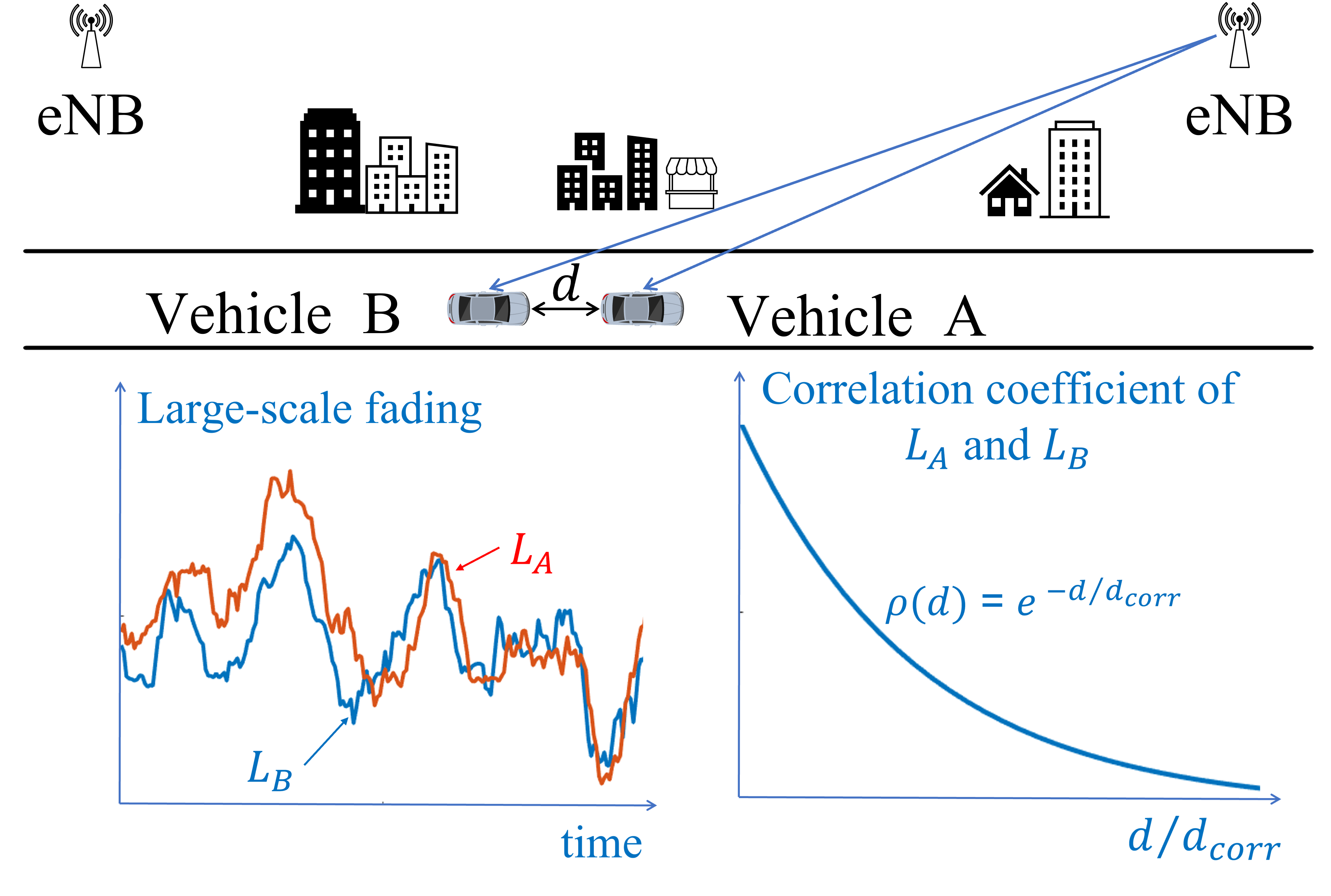
Experimental validation. To validate the spatial and temporal correlation properties of large-scale fading, we collected measurements of LTE signals in a freeway environment, which is the most relevant for platooning applications. The data was collected by driving a platoon of two vehicles and and simultaneously measuring the RSS (Note that, since RSS (in dB) is the difference between the transmit power and path loss, measuring RSS is equivalent to measuring the fading). from eNBs. The location and timestamp of each sample was also recorded to allow for time sample alignment and the computation of the separation Figure 4 shows the topology used in the experiments, along with a sample realization of the measured large scale fading samples and the correlation model in eq. (2). The experimental setup is described in detail in Sec. V-A. We tested the following two main hypotheses.
-
1.
Spatial correlation decreases with distance. Here, we seek to verify the correlation model in [12] and determine the decorrelation distance .
-
2.
Temporal correlation decreases with time. Here, we seek to verify that the correlation of RF signals collected at the same location but different times decreases with the time difference.

To extract the large-scale fading and filter out the small-scale fading, we apply an -point moving RSS average . We then compute the Pearson’s correlation coefficient as the correlation metric, defined as:
| (3) |
where and are the mean values of the RSS moving average over RSS entries for and , respectively.
IV-B1 Spatial Correlation Decreases with Distance
To validate this hypothesis, two vehicles were driven with following distance on a freeway at 30mph. A total of 6,000 samples were collected at a sampling rate of 20Hz for each (5 min duration). The samples were organized to subsets of 1,200 samples (1 min duration) and the correlation was computed over each subset, using a 40-point moving average.
Figure 5 shows the correlation averaged over all subsets, as a function of the vehicle separation The fitting of the theoretical curve obtained from the exponential model in (2) yielded a decorrelation distance . This is in the same order of a typical platooning distance bound, indicating that correlation would be an ideal metric to implement the PoF primitive. Note that although the average correlation fits to a deterministic model, the RSS samples used to compute the correlation are constantly changing with mobility and have high entropy (which we will show in Appendix A).
IV-B2 Temporal correlation decreases over time
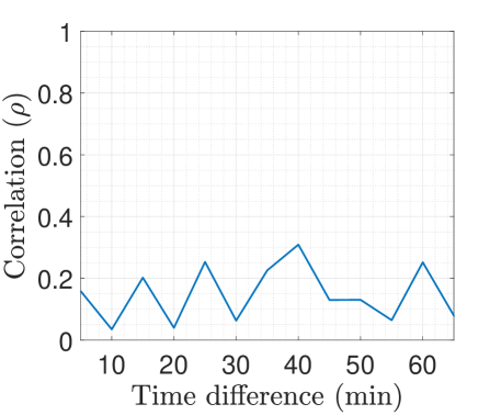
To validate the temporal decorrelation hypothesis, we collected LTE transmission samples over the same route but at different times. We drove vehicle and platooning over the same freeway segment and computed the correlation between samples collected by the two vehicles, but aligned to the same locations. That RSS samples aligned to the same location but different time, where the difference equals the time separation of the two vehicles. The two vehicles were moving at 30Mph and had fixed time difference from 1s to 9s (13m to 112m). Due to the absence of CACC, fixed separation was achieved by engaging the cruise control on both vehicles and performing many trial runs. Figure 6(a) shows the correlation as a function of the time difference between sampling of the same location. We observe that the temporal correlation drops to fairly low values after a few seconds. This is an important property to prevent pre-recording attacks, where the adversary traverses the platoon route ahead of time to collect historic RSS data and use these data to defeat a PoF verification. Figure 6(b) shows the temporal correlation for a longer timescale.
From the experimental evaluation of the the spatial and temporal correlation of the large-scale fading effect, we can conclude that it is a good candidate to differentiate a following vehicle as drops to low values for separations larger than the platooning distance (beyond 50m) and also remains low between samples collected at even just a few seconds apart (this is inline with the typical channel coherence time of outdoor channels for large-scale fading).
 |
 |
| (a) short time scale | (b) long time scale |
IV-C Proof-of-Following Protocol
IV-C1 Overview
The high level idea of our PoF protocol is to compute the correlation between the smoothed RSS samples gathered by the candidate and verifier (corresponding to large-scale fading), and compare it with a threshold . Suppose the correlation function follows the deterministic model in Eq. (2), given a required distance threshold , setting will make all vehicles following within pass the PoF test () and all others will fail. However, the correlation model expressed in Eq. (2) is for the average correlation, and in practice certain correlation instances will fluctuate around the average, due to changes of the environment/terrain as vehicles move. A single test designed according to the correlation model will only provide a weak probabilistic guarantee for passing or failing the test at different distances (the CDF of the correlation would be required). Thus, we opted to organize the RSS data in shorter correlation tests instead of a single long test. Repeated tests is a standard mechanism for driving the adversary’s probability of passing verification towards zero.
IV-C2 Protocol Details
A PoF consists of four phases, namely initialization, collection, PoF verification, and continuous following verification. The steps of the PoF are shown in Fig. 7. Note that knows a priori which platoon he is going to join. We treat the case of an unknown verifier with an amended PoF protocol to account for MiTM attacks. To facilitate platoon discovery, the verifier periodically broadcasts its ID along with his credentials (public key and certificate).
Initialization phase.
-
1.
Candidate sends a platoon join request message REQ to the verifier . The message is signed with and then encrypted with The candidate prepends the verifier’s ID to REQ.
-
2.
The verifier decrypts the message with and verifies the signature with . If verification passes, triggers a proof-of-following verification by sending a reply message REPLY. The message is signed with and then encrypted with The message also contains a) the start and end times of RSS sampling, and b) the sampled frequency and sampling rate.
-
3.
decrypts and verifies the signature of It then records the start and end times of the collection phase. Loose clock synchronization is achieved via the GPS clocks.
Collection phase. In this phase, and sample a common frequency between the start and end times.
-
4.
The verifier and the candidate simultaneously collect RSS samples and , respectively.
where is the RSS sample collected by vehicle at time .
-
5.
The candidate reports his recording to the verifier signed and encrypted. The verifier decrypts and verifies the signature. If verification passes, it moves to the PoF verification phase.
PoF verification phase. In this phase, verifies the “following” claim of the candidate by computing the RF correlation between the reported RSS measurements and its own recorded measurements .
-
6.
The verifier aligns and using the respective timestamps. This is done by aligning the first sample (the two vehicles use the same sampling rate). then updates the RSS sets and to
where each is time-aligned with sample
-
7.
The verifier separates and into subsets of size samples. Let denote the -th subset of set .
-
8.
The verifier computes the correlation for the subsets and for using eq. (3). The verifier obtains correlation values
-
9.
The verifier compares each correlation value with a passing threshold . if a fraction () of correlation values exceed the passing threshold , the verifier ACCEPTS. Otherwise, the verifier REJECTS. That is, the verification test is passed if
where is the indicator function.
Continuous following verification phase.
-
10.
If the candidate passes the PoF verification, it is accepted in the platoon. Continuous following verification can be achieved by repeating the collection and verification phases continuously.
| Candidate | Verifier | |
| Given: | ||
| Parameters (, , , , ) | ||
| Initialization: | ||
| Decrypt: , REQ, | ||
| Verify: | ||
| Verify: | ||
| Decrypt: , REPLY, | ||
| Verify: | ||
| Collection: | ||
| SYNC | ||
| Collect | Collect | |
| Decrypt: , , | ||
| Verify: | ||
| Record | ||
| Verification: | ||
| Align , , | ||
| Form , , | ||
| Compute {}, | ||
| Verify: | ||
| Continuous following verification: | ||
| Repeat collection and verification |
IV-D Security Analysis
In this section, we analyze the security of our PoF protocol against different types of adversaries.
IV-D1 Remote and Following-afar Adversaries
A remote or following-afar adversary can request to join a platoon represented by verifier by sending a join request
|
|
The verifier verifies the identity of (by verifying the public key using the certificate and sends REPLY to which also indicates the start and end times of the RSS collection, as well as the probed frequency. At this point, the adversary has two choices: (a) to use RSS data that is pre-recorded on the path traveled by the platoon, or (b) to collect real time data at his current location (for the following-afar adversary). Then sends
to for authentication. To pass the PoF verification, the set provided by must satisfy the correlation test applied by However, since is not within the following distance or was collected a long time before , the two RSS data sets decorrelate according to Eq. (2) and Fig. 6. So both remote adversary and following-afar adversary will be rejected. We experimentally evaluate the correlation achieved at different distances and for different environments in Sec.V.
IV-D2 Partially-following Adversary
A partially-following adversary can similarly initiate the PoF process by sending an message to . It can pass a fraction of tests when it is within following distance but fail the rest of tests when he moves far from . The fraction of correlation tests passed by the adversary depend on the fraction of time that follows Theoretically, if the adversary is within a following distance for a fraction of the RSS collection time, then he should pass a fraction of the tests, thus being admitted in the platoon. In practice, a larger fraction of time may be needed because some tests fail even for valid candidates due to the RSS randomness. In Sec. V-F, we evaluate the passing rate of a partially following adversary in our experimental setting. Note that when continuous authentication is employed, the partially-following adversary has to periodically approach to be retained as a platoon member.
IV-D3 MiTM Attacks
In a MiTM attack, the adversary attempts to be admitted to the platoon when a valid candidate initiates a join request with the verifier. The adversary is not within following distance of . We analyze two instances of the attack. In the first instance, is aware of the verifier that he attempts to join. This is implied in our PoF protocol, as and are given to according to the assumptions we have made for the PoF protocol (see Fig. 7). We further treat the case where the candidate does not know the verifier a priori, but responds to a broadcast of a nearby verifier.

Known verifier. Let be given to via some out-of-band channel before the PoF protocol execution (e.g., is instructed to join a specific ). In this case, spurious forwarding from a MiTM adversary is prevented by the authenticated encryption used to transmit the RSS value set to the verifier. For ease of illustration, Figure 8 demonstrates a possible MiTM attack. Let the candidate initialize the protocol by sending the join request message Note that is encrypted with so only can decrypt it. The adversary can attempt to initiate parallel sessions by eliminating from the channel and injecting his own message
to the verifier. After receiving the reply , if the adversary replaces with his own message
will abort because the signature verification will fail ( expects a message signed by and verified with ). Alternatively, can relay and move forward to the stage of transmitting the collected RSS sets. Upon collection of , the candidate sends message
which is intercepted by . Because is encrypted with ’s public key, cannot recover As a result, fails to construct message that would contain ’s RSS samples. The only recourse is to include his own samples which are not correlated with ’s samples, as is beyond the following distance, leading to a REJECT by the verifier.
Unknown verifier. If the verifier’s identity is not known to a priori, the candidate must undergo a discovery phase to probe for nearby verifiers. This scenario is relevant when vehicles are forming platoons in an ad hoc manner to improve fuel efficiency and safety, without necessarily belonging to the same organization. If the verifier is unknown, can launch a spoofing attack on and convince him that is a valid verifier. At the same time can open a parallel session with the legitimate , requesting to join the platoon. The candidate will provide with his RSS set , which can immediately use to pass the RSS correlation test at
To prevent a MiTM attack, we amend our PoF protocol to include a commitment scheme [13] with a delayed opening phase that renders the RSS samples obtained by the adversary stale. The key idea is rather than revealing the RSS samples, presents a commitment on those samples to the verifier. The commitment is opened with a delay to complete the PoF verification. A MiTM adversary spoofing a verifier cannot open the commitment of due to the hiding property. The delayed opening phase forces to commit without knowing or commit late with RSS samples that are not aligned with those of Thus, will reject ’s join request. Due to space limitations, we present the amended PoF protocol and a detailed security analysis in Appendix -A.
IV-D4 Mutual PoF Verification
We emphasize that our PoF protocol does not provide any proof of platooning to the candidate, as it implements access control to existing platoons. This opens the possibilities for verifier spoofing where the candidate may join a verifier that he does not follow. This type of attack can be thwarted by extending the delayed commitment scheme in both directions. The verifier would also be required to commit to its own RSS samples and reveal them in a delayed opening phase.
V Evaluation
In this section, we evaluate the correctness and soundness of the PoF. We describe our experimental testbed, we demonstrate how to select the test parameters, and present experimental results in freeway, urban, and highway environments.
V-A Testbed
We developed two setups based on the NI USRP platform [1]. The first setup was employed in the freeway and urban driving experiments whereas the second setup was employed in the highway driving experiments.
Setup 1. We used a Nissan Sentra and a BMW X5 acting as and , respectively. The two vehicles had cruise control capabilities (not adaptive), but were otherwise manually operated. We placed at the trunk of each vehicle the equipment shown in Fig. 9. A USRP N200 radio device was connected to a VERT900 antenna. The USRP was programmed to implement an OFDM receiver for LTE signals. It operated at 1.972GHz with a 4MHz bandwidth, which is the frequency used for personal communications service (PCS) in LTE. We set the gain of the antenna to 10dB and the sample rate to 20Hz. A Razer blade stealth laptop was connected to the USRP for recording the RSS data. The laptop was also connected to a GPS receiver to record positioning information at 5Hz sampling rate. The synchronization between the RSS and GPS data was achieved via the laptop clock.
Setup 2. In setup 2, we formed a two-vehicle platoon for driving in a highway environment. Here, (Honda Pilot) led the platoon with cruise control engaged, whereas (Toyota RAV-4) followed with adaptive cruise control engaged. The candidate was equipped with a LiDAR to measure the distance to . This allowed for an easier and more accurate control of the separation distance between the two vehicles at highway speeds. Although setup 2 is superior to setup 1 from a platooning perspective, it was not always available to us to conduct the experiments that spanned many hours and days, so we limited it to highway experiments were maintaining constant distance presents more challenges. The data collection setup was identical to that of Setup 1, with the central frequency set to 875MHz with 4 MHz bandwidth and the antenna gain was 20 dB. The new frequency was selected based on the signal availability at the specific part of the highway were experiments were conducted.

 |
 |
 |
 |
| (a) | (b) | (c) | (d) |
V-B PoF Test Parameter Selection
The PoF test is controlled by the selection of the , , , , and parameters. For clarity, we summarize the definition of these parameters in Table I. In this section, we show how to select the parameter in practice and then evaluate the PoF protocol in three driving environments.
To select and , we performed experiments on a freeway section of length 1.4 miles using Setup 1. The particular section was not accessible to other traffic and was located next to a highway. This presented an ideal situation for safely controlling the following distance. The two vehicles were driven at 30Mph over multiple runs and at different following distances. We collected RSS data using the radio testbed and processed the collected data using various test parameters.
Selecting . The subset size determines the number of samples used per correlation test. It must be long enough to ensure that RSS values exhibit high correlation, but should not prolong the test duration. We experimented with different lengths . For each , we reused the second-half samples in each subset to form the first-half samples for the following subset to reduce the test duration. Figure 10(a) shows as a function of the following distance . Generally, when a larger is selected, the correlation increases (except for ranges over 90m where the two RSS sequences are uncorrelated). From Fig. 10(a), we can see that beyond the gains in correlation are relatively small. Therefore, we fix for all the following evaluations.
| Notation | Definition |
|---|---|
| Number of samples in subsets and | |
| Moving average window size | |
| Number of RSS subsets, correlation values, and correlation tests | |
| Passing threshold for a single correlation test | |
| Fraction of correlation tests to pass PoF verification | |
| Passing rate of a single correlation test achieved by | |
| Passing rate of correlation tests achieved by |
Selecting . The length of the moving average window impacts the elimination of small-scale fading. Intuitively, a larger window leads to a more stable moving average, and a higher correlation , but the moving average becomes more predictable. In Fig. 10(b), we show the correlation as a function of the following distance for different . As expected, we observe an increase in correlation with at short distances, whereas the impact of is small for large distances because the two RSS sequences are uncorrelated. Moreover, the increase in correlation diminishes after . Based on these observations, we set .
Selecting , , and . Let denote the probability of passing a single correlation test when an RSS subset is used to compute . This probability depends on the selection of and the following distance . For a total of tests, a PoF is passed if Assuming independent tests due to the use of different subsets, the probability of passing a PoF verification consisting of correlation tests is
| (4) |
where is the binomial coefficient. Let denote the probability of passing the PoF verification for and to be the passing probability for . Probability is derived from Eq. (4) by substituting the probability of passing a single correlation test at , given the selection of Similarly, is derived from Eq. (4) by substituting the probability of passing a single correlation test at some distance , The equal error rate () is defined as
| (5) |
We aim at selecting that minimizes the . To understand the interplay between , and , we generated the PDF of the correlation for three representative following distances. The respective PDFs are shown in Fig. 10(c). From the PDF, one can select a desired to satisfy a required passing rate for valid candidates for a given For instance, we chose for and for A is representative of a following-afar adversary.
Given , we performed an exhaustive search over the two remaining free variables and to minimize the Here, we limit to 40 to ensure that a PoF test adheres to a time limit and also limited such that takes integer values between 1 and . Figure 10(d) shows the as a function of when the optimal is selected. As expected, the decreases with . Here, a that satisfied a desired requirement can be selected at the expense of a PoF test duration. For the freeway experiments, we set
An alternative method for selecting and under fixed is to first determine two following distances from the platooning requirements. The first distance is that of the valid candidate, namely , whereas the second is that of the afar adversary that we try to prevent against. We then compute the threshold for a single correlation test from the exponential model in Eq. (2) by setting . Once is fixed, we select to maximize the gap between and . Given that the average correlation model may not hold for all driving environments, we opted to use the exhaustive search method to explore the performance of the PoF. These methods require the use of at least one trusted vehicle besides the verifier in the platoon to calculate passing rate . If there is only one vehicle in the platoon, has to select from eq. (2). Except , all other parameters () can be preset since they are stable in different environments.
V-C Evaluation of PoF on the Freeway
For the freeway experiments, we employed Setup 1, with the two vehicles driving at approximately at 30Mph. Because the specific freeway section was closed, we were able to control the following distance between the two vehicles. We drove the vehicles at following distances between 10m - 115m.
Based on the parameter selection we discussed in the previous section, we set , and We then performed an exhaustive search to find the optimal threshold values and that minimize the Figure 11 shows the minimum EER for different values of valid following distance when the adversary follows at 90m. The optimal values of and that minimize the for each following distance are also shown. First, we observe that our method achieves a fairly low . Moreover, the optimal and do not vary significantly with the change of
In Fig. 12, we show the PoF passing rate as a function of the following distance for the optimal and values obtained from minimizing the . When a candidate is within a following distance between 10m-40m the passing rate is close to 1. The passing rate drops to zero for distances larger than 90m. The method leaves a “guard” zone between 40-90 where the passing rate is from 0.2 to 0.4. This zone cannot be considered to be secure as an adversary following in this zone could pass a PoF test with non-negligible probability. This is because the correlation degrades gracefully with distance and does not exhibit a step-function type of behavior.


Ideally, for any environment, we estimate the distribution of with different distance, and set . However, in practice, the distance between two vehicles is difficult to control due to the traffic, especially in urban and highway areas, which thwarts us from selecting with CDF of . Instead, we are interested in evaluating PoF for certain given distance bound, from which we select based on the statistically relationship between the passing rate of a single correlation and the threshold . After that, and can be chosen with minimum . For all the following results, we also use 30 of experimental data as a training sequence for parameter selection, and the remaining 70 for testing.
 |
 |
 |
 |
| (a) urban | (b) urban | (c) highway | (d) highway |
 |
| (a) urban |
 |
| (b) highway |
V-D Evaluation of PoF in an Urban Area
For the urban area experiments, we used Setup 1 to drive the two vehicles along a 2.5-mile route inside Tucson city from River to Grant road, as shown in Fig. 14(a), several rounds for one hour. Except stops at red lights, the vehicles normally run at a speed up to 40Mph and always followed each other. Figure 13(a) shows the following distance over time. The following distance was fairly stable with an average of about 11 meters. Since the mixed traffic did not allow us to precisely control the following distance , we did not obtain the PDF of the correlation for different distances as we did for the freeway experiments. Thus, we select optimal values of , , and by minimizing the .
V-D1 Parameter Selection
Selecting . According to Sec. IV-B, the single test passing rates for and should satisfy and , respectively. To select the threshold , we first plot and as functions of the single test correlation threshold , based on our experimental data (Fig. 15(a)). From this we set the range of to be , in order to satisfy and .
Selecting and . Recall that we use tests and fraction of passing to drive the probability of successful verification for the candidate vehicle and an adversary to one and zero, respectively. In Fig. 15(b), we show the minimum for against the corresponding , Values of are shown in Fig. 15(c). We can see that with the corresponding and minimize the .
V-D2 Remote adversary
In the following, we show results for a remote adversary, who pre-records RSS data on the known platoon route and replays it to pass the PoF verification. We let the Nissan Sentra serve as a remote adversary by prerecording RSS for 70 minutes ahead on the same route of the platoon. Then the selected parameters above are used in all PoF verification test sets. Each test set will output accept or reject after 19 correlation tests. We run the PoF tests for multiple times (continuous verification) and calculated the PoF test passing rate. In Fig. 15(d), we show the PoF passing rate versus the number of correlation tests . For each , the PoF passing rate was computed over 10 PoF runs. We observed that the PoF passing rate for increases with the number of correlation tests, while it decreases for . After 19 correlation tests, achieved PoF passing rate, and the verifier rejected the adversary (). This shows that in an urban environment, our PoF protocol can successfully differentiate a legitimate candidate from a remote adversary.
V-D3 Following-afar adversary
We further evaluated the following-afar adversary model, when tries to pass verification by transmitting real-time recorded RSS data. This adversary was realized by driving at least 125 meters behind Due to the presence of traffic lights on the city streets, the distance between and varied during the experiment, as shown in Fig. 13(b), with 125 meters being the average.
 |
 |
 |
 |
| (a) | (b) | (c) | (d) |
We selected the parameters with training sets collected by a following-afar model following the same steps as in Sec. V-D1, and show the details in Fig. 16(a)-(c). Similarly, we plot the PoF passing rate for and over 15 PoF verifications in Fig. 16(d). Again, we can see that the PoF is secure against the following-afar adversary.
 |
 |
 |
 |
| (a) | (b) | (c) | (d) |
V-E Evaluation of PoF on the Highway
We ran experiments on a highway environment using Setup 2. Two platooning vehicles were driven on the piece of I-10 highway, shown in Fig. 14(b), from exit 250 to 257 for 6.4-mile back and forth over a period of 1.5 hours. The distance between and was maintained using ACC and remained quite stable (see Fig. 13(c)), with a 53.4m average.
V-E1 Remote adversary
We drove the Nissan Sentra to pre-record the RSS on the same route as the legitimate platoon. Due to the high speed on the highway, the channel varied much more rapidly compared to urban areas. Therefore, for this experiment, we pre-recorded the RSS data 40 minutes ahead of time to mimic a remote adversary. The results for parameter selection were plotted in Fig. 18(a)-(c), where we selected , and . In Fig. 18(d), we showed the convergence curve of PoF passing rate for both and over 13 PoF runs, where the legitimate candidate was verified with certainty for and the remote adversary was always detected for , respectively.
V-E2 Following-afar adversary
Next, we evaluated the following-afar adversary. The adversary followed the verifier at a distance of at least 100m. The following distance trace is shown in Fig. 13(d). The average following distance was 250m and varied significantly due to heavy highway traffic. The results of parameter selection are shown in Fig. 19(a)-(c). We selected , , and . The PoF passing rate averaged over 10 runs is shown in Fig. 19(d), where we observe that and when and , respectively. We can see that the PoF yields better performance against the following-afar adversary (lower EER and faster PoF passing rate) than the remote adversary, mainly because the distance between the verifier and the adversary is larger in the highway and vehicles travel at high speeds.
V-F Evaluation of PoF against Partially-following Adversary
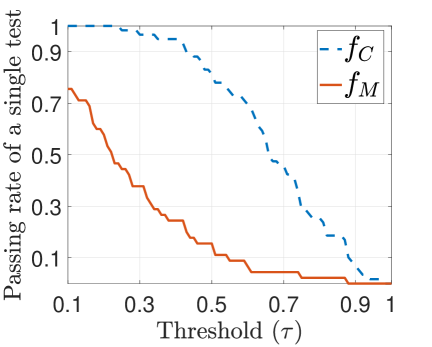
We further implemented a partially-following adversary who was within following distance for a fraction of a PoF duration, whereas he remained outside the following distance for the remaining PoF time. In Fig. 17, we show the PoF passing rate as a function of . The test parameters () were set to the values indicated in Sec. V-D for the urban environment and Sec. V-E for the highway environment, assuming a following-afar adversary. The passing rates are averaged over 11 PoF runs for the urban and 13 runs for the highway environment, respectively. We observe that to pass the authentication with non-zero probability, the adversary has to follow the platoon at least 50% of the PoF duration (in the order of 100 seconds). For the urban environment where the RSS fluctuates more rapidly, the adversary is guaranteed to pass the PoF (passing rate equal to one) if he follows 90% of the time, whereas this percentage drops to around 70% on the highway environment. This indicates that a partially-following adversary could be successful, if he dedicates a significant portion of time in truly following the verifier.
 |
 |
| (a) urban | (b) highway |
V-G Evaluation of RSS Randomness
Another approach for a remote adversary is to predict real-time RSS data from pre-recorded data. We use approximate entropy to evaluate the randomness of the moving average values used to compute the correlation. Approximate entropy is preferred to sample entropy because it is a more accurate randomness measure when the number of samples is limited [29]. We calculate the approximate entropy of following standard steps in [48, 29]. For the two parameters and required for approximation entropy calculation (i.e., the length of compared run of data and the similarity criterion, respectively), we use typical values and as done in [29], where is the standard deviation of . The for the urban and highway environment is 0.4730 and 0.3088, respectively. The of a perfectly repeatable time series is about 0 [48], and is around 0.6 for binary expansions of some common irrational numbers [32]. Hence, our results indicated that the large-scale fading in dynamic traffic is random and unpredictable enough. Furthermore, it would be difficult for the attacker to pass the verification by predicting the RSS measurement of verifier .
 |
 |
 |
 |
| (a) | (b) | (c) | (d) |
 |
 |
 |
 |
| (a) | (b) | (c) | (d) |
V-H Duration of the PoF Protocol
The duration of each PoF protocol is dominated by the RSS collection phase. The number of the RSS samples needed for the test is decided by the parameters we select. Since we reuse RSS samples for two consecutive subsets, it requires RSS samples to complete correlation tests, which takes seconds for data collection. For the urban and highway environments, we fixed , , and our sampling rate was 20Hz. Therefore, about 200 seconds are required for each PoF protocol run. This is a reasonable cost as vehicle platoons are intended to travel for relatively long periods of time.
VI Future Directions
Verification of other physical properties. Our current PoF construct verifies continuous following within the following distance. For strict platooning verification relative vehcile positioning and lane restrictions shall also be verified. To verify the relative position, we can leverage two vehicles already accepted by the platoon. Assume vehicle wishes to prove it is located between and , then can send its RSS samples to both and . If is following behind and , this can also be proved if is in the range of but not or by repeating tests with different .
Verifying traveling on the same lane is more challenging. In the RF domain, one can use features such as the angle-of-arrival (AoA) and Doppler shift. With multi-antenna receivers that may be standard with the advent of 5G, a verifier can determine the candidate’s AoA using beamforming. If the candidate is in the same lane, the AoA is either or . AoA has been previously used to enhance WiFi security [47], as well as for secure motion verification [39]. It is difficult to spoof without deploying artificial reflectors. A high mobility scenario makes it nearly impossible. If only a single-antenna transceiver is available, one can exploit the Doppler shift (DS) which reflects the relative speed. If the candidate follows the verifier closely at the same speed and lane, he should measure similar DS from V2V signals from other vehicles. Any vehicle on another lane would not measure the same DS due to different angles.
PoF from other sensing modalities. Cameras can also be used to capture the ambient physical environment as the platoon travels on the road. Imagine a verifier and a candidate traveling on the same highway. Using cameras, they can capture, analyze, and cross-correlate images of transient environment features. For instance, the two vehicles could capture and timestamp images of a passing by semi-truck (moving element) with some static feature in the background (building, tree, billboard, etc). This will ensure that the two vehicles are co-traveling within the following distance.
Another approach is to measure the following distance using LiDAR. The verifier could randomly perturb the following distance by subtly accelerating and braking. A valid candidate should be able to accurately measure the distance changes and report them to the verifier. If both parties agree on the perturbations, the PoF test is passed. We will explore these extensions in our future works.
VII Conclusion
We proposed a novel security primitive called Proof-of-Following (PoF) that binds the physical property of “following” to the candidate vehicle’s digital identity. Our PoF protocol allows a candidate vehicle to continuously prove to a verifier vehicle that it follows the verifier within the typical platooning distance. We exploited the large-scale wireless fading from cellular towers as an easy-to-measure solution correlating the motions of vehicles. Our approach has a remarkable advantage in hardware requirements as only the RF modality is required, which is widely available in outdoor environments. We conducted extensive real-world experiments in the freeway, urban and highway environments to evaluate the performance and security of our PoF protocol. Results showed that PoF is resistant to both pre-recording and following attacks with overwhelming probability and robust performance.
Acknowledgements
We thank the anonymous reviewers for their insightful comments. We also like to thank Dr. Jonathan Sprinkle and Dr. Matt Bunting for their help with the highway experiments. This work was supported by ARO grant W911NF-19-1-0050.
References
- [1] [Online]. Available: https://www.ettus.com
- [2] 3GPP. Testing C-V2X access layer for its devices. [Online]. Available: https://www.3gpp.org/news-events/2120-c-v2x
- [3] 3rd Generation Partnership Project;Technical Specification Group Services and System Aspects;Security aspect for LTE support of Vehicle-to-Everything (V2X) services Rel-16, V16.0.0, 3GPP Std. TS 33.185, Jul. 2020.
- [4] A. Algans, K. I. Pedersen, and P. E. Mogensen, “Experimental analysis of the joint statistical properties of azimuth spread, delay spread, and shadow fading,” IEEE Journal on Selected Areas in Communications, vol. 20, no. 3, pp. 523–531, 2002.
- [5] G. Avoine, M. A. Bingöl, I. Boureanu, S. čapkun, G. Hancke, S. Kardaş, C. H. Kim, C. Lauradoux, B. Martin, J. Munilla, A. Peinado, K. B. Rasmussen, D. Singelée, A. Tchamkerten, R. Trujillo-Rasua, and S. Vaudenay, “Security of distance-bounding: A survey,” ACM Comput. Surv., vol. 51, no. 5, Sep. 2018.
- [6] Y. Bian, Y. Zheng, W. Ren, S. E. Li, J. Wang, and K. Li, “Reducing time headway for platooning of connected vehicles via V2V communication,” Transportation Research Part C: Emerging Technologies, vol. 102, pp. 87–105, 2019.
- [7] N. Bißmeyer, J. Njeukam, J. Petit, and K. M. Bayarou, “Central misbehavior evaluation for vanets based on mobility data plausibility,” in Proc. of VANET, 2012, pp. 73–82.
- [8] S. Brands and D. Chaum, “Distance-bounding protocols,” in Workshop on the Theory and Application of of Cryptographic Techniques. Springer, 1993, pp. 344–359.
- [9] M. Conti and C. Lal, “Context-based co-presence detection techniques: A survey,” Computers & Security, vol. 88, p. 101652, 2020.
- [10] K. Guan, B. Ai, Z. Zhong, C. F. López, L. Zhang, C. Briso-Rodríguez, A. Hrovat, B. Zhang, R. He, and T. Tang, “Measurements and analysis of large-scale fading characteristics in curved subway tunnels at 920 MHz, 2400 MHz, and 5705 MHz,” IEEE Transactions on Intelligent Transportation Systems, vol. 16, no. 5, pp. 2393–2405, 2015.
- [11] J. Guanetti, Y. Kim, and F. Borrelli, “Control of connected and automated vehicles: State of the art and future challenges,” Annual Reviews in Control, vol. 45, pp. 18–40, 2018.
- [12] M. Gudmundson, “Correlation model for shadow fading in mobile radio systems,” Electronics Letters, vol. 27, no. 23, pp. 2145–2146, 1991.
- [13] S. Halevi and S. Micali, “Practical and provably-secure commitment schemes from collision-free hashing,” in Annual International Cryptology Conference, 1996, pp. 201–215.
- [14] J. Han, A. J. Chung, M. K. Sinha, M. Harishankar, S. Pan, H. Y. Noh, P. Zhang, and P. Tague, “Do you feel what I hear? enabling autonomous iot device pairing using different sensor types,” in 2018 IEEE S&P, pp. 836–852.
- [15] J. Han, M. Harishankar, X. Wang, A. J. Chung, and P. Tague, “Convoy: Physical context verification for vehicle platoon admission,” in Proc. of HotMobile, 2017, pp. 73–78.
- [16] E. Hayashi, S. Das, S. Amini, J. Hong, and I. Oakley, “Casa: context-aware scalable authentication,” in Proc. of SOUPS, 2013, pp. 1–10.
- [17] R. He, Z. Zhong, B. Ai, and C. Oestges, “Shadow fading correlation in high-speed railway environments,” IEEE Transactions on Vehicular Technology, vol. 64, no. 7, pp. 2762–2772, 2014.
- [18] IEEE Standard for Wireless Access in Vehicular Environments (WAVE)–Certificate Management Interfaces for End Entities, IEEE Std. IEEE 1609.2.1, 2020.
- [19] D. Jia, K. Lu, J. Wang, X. Zhang, and X. Shen, “A survey on platoon-based vehicular cyber-physical systems,” IEEE communications surveys & tutorials, vol. 18, no. 1, pp. 263–284, 2015.
- [20] M. Juuti, C. Vaas, I. Sluganovic, H. Liljestrand, N. Asokan, and I. Martinovic, “Stash: Securing transparent authentication schemes using prover-side proximity verification,” in IEEE SECON, 2017, pp. 1–9.
- [21] J. Kamel, M. R. Ansari, J. Petit, A. Kaiser, I. B. Jemaa, and P. Urien, “Simulation framework for misbehavior detection in vehicular networks,” IEEE Transactions on Vehicular Technology, vol. 69, no. 6, pp. 6631–6643, 2020.
- [22] B. Ko and S. H. Son, “An approach to detecting malicious information attacks for platoon safety,” IEEE Access, vol. 9, pp. 101 289–101 299, 2021.
- [23] X. Li, Q. Zeng, L. Luo, and T. Luo, “T2pair: Secure and usable pairing for heterogeneous iot devices,” in Proc. of CCS, 2020, pp. 309–323.
- [24] D. L. Luu, C. Lupu, L. S. Ismail, and H. Alshareefi, “Spacing control of cooperative adaptive cruise control vehicle platoon,” in Proc. of IEEE AQTR, 2020, pp. 1–6.
- [25] N. Lyamin, Q. Deng, and A. Vinel, “Study of the platooning fuel efficiency under ETSI ITS-G5 communications,” in Proc. of IEEE 19th ITSC, 2016, pp. 551–556.
- [26] S. Mathur, R. Miller, A. Varshavsky, W. Trappe, and N. Mandayam, “Proximate: proximity-based secure pairing using ambient wireless signals,” in Proc. of MobiSys, 2011, pp. 211–224.
- [27] M. Miettinen, N. Asokan, T. D. Nguyen, A.-R. Sadeghi, and M. Sobhani, “Context-based zero-interaction pairing and key evolution for advanced personal devices,” in Proc. of CCS, 2014, pp. 880–891.
- [28] V.-L. Nguyen, P.-C. Lin, and R.-H. Hwang, “Enhancing misbehavior detection in 5G vehicle-to-vehicle communications,” IEEE Transactions on Vehicular Technology, vol. 69, no. 9, pp. 9417–9430, 2020.
- [29] S. M. Pincus, “Approximate entropy as a measure of system complexity,” Proc. of the National Academy of Sciences, vol. 88, no. 6, pp. 2297–2301, 1991.
- [30] I. Qualcomm Technologies. Connecting vehicles to everything with C-V2X. [Online]. Available: https://www.qualcomm.com/research/5g/cellular-v2x
- [31] I.-R. Recommendation, “Guidelines for evaluation of radio transmission technologies for IMT-2000,” Rec. ITU-R M. 1225, 1997.
- [32] A. L. Rukhin et al., “Approximate entropy for testing randomness,” Journal of Applied Probability, vol. 37, no. 1, pp. 88–100, 2000.
- [33] D. Schürmann and S. Sigg, “Secure communication based on ambient audio,” IEEE TMC, vol. 12, no. 2, pp. 358–370, 2011.
- [34] G. Senarath, “Multi-hop relay system evaluation methodology (channel model and performance metric),” http://ieee802. org/16/relay/docs/80216j-06_013r3. pdf, 2007.
- [35] L. Shi, M. Li, S. Yu, and J. Yuan, “Bana: Body area network authentication exploiting channel characteristics,” IEEE Journal on Selected Areas in Communications, vol. 31, no. 9, pp. 1803–1816, 2013.
- [36] S. So, J. Petit, and D. Starobinski, “Physical layer plausibility checks for misbehavior detection in V2X networks,” in Proc. of WiSec, 2019, pp. 84–93.
- [37] M. Song, F. Chen, and X. Ma, “Organization of autonomous truck platoon considering energy saving and pavement fatigue,” Transportation Research Part D: Transport and Environment, vol. 90, p. 102667, 2021.
- [38] M. Sun, M. Li, and R. Gerdes, “A data trust framework for vanets enabling false data detection and secure vehicle tracking,” in Proc. of CNS. IEEE, 2017, pp. 1–9.
- [39] M. Sun, Y. Man, M. Li, and R. Gerdes, “SVM: secure vehicle motion verification with a single wireless receiver,” in Proc. of WiSec, 2020, pp. 65–76.
- [40] S. S. Szyszkowicz, H. Yanikomeroglu, and J. S. Thompson, “On the feasibility of wireless shadowing correlation models,” IEEE Transactions on Vehicular Technology, vol. 59, no. 9, pp. 4222–4236, 2010.
- [41] N. O. Tippenhauer, H. Luecken, M. Kuhn, and S. Capkun, “UWB rapid-bit-exchange system for distance bounding,” in Proc. of WiSec, 2015, pp. 1–12.
- [42] V. Turri, B. Besselink, and K. H. Johansson, “Cooperative look-ahead control for fuel-efficient and safe heavy-duty vehicle platooning,” IEEE Transactions on Control Systems Technology, vol. 25, no. 1, pp. 12–28, 2016.
- [43] Automated Vehicles Comprehensive Plan, U.S. Department of Transportation, Washington, DC, USA, 2021. [Online]. Available: https://www.transportation.gov/sites/dot.gov/files/2021-01/USDOT_AVCP.pdf
- [44] C. Vaas, M. Juuti, N. Asokan, and I. Martinovic, “Get in line: Ongoing co-presence verification of a vehicle formation based on driving trajectories,” in Proc. of the IEEE EuroS&P, 2018, pp. 199–213.
- [45] G. Wood, “Truck platooning expected to make inroads in 2020,” https://www.oemoffhighway.com/electronics/smart-systems/automated-systems/article/21114230/truck-platooning-expected-to-make-inroads-in-2020.
- [46] Y. Wu, A. Khisti, C. Xiao, G. Caire, K.-K. Wong, and X. Gao, “A survey of physical layer security techniques for 5G wireless networks and challenges ahead,” IEEE Journal on Selected Areas in Communications, vol. 36, no. 4, pp. 679–695, 2018.
- [47] J. Xiong and K. Jamieson, “SecureArray: Improving WiFi security with fine-grained physical-layer information,” in Proc. of MobiCom, 2013, pp. 441–452.
- [48] J. M. Yentes, N. Hunt, K. K. Schmid, J. P. Kaipust, D. McGrath, and N. Stergiou, “The appropriate use of approximate entropy and sample entropy with short data sets,” Annals of Biomedical Engineering, vol. 41, no. 2, pp. 349–365, 2013.
- [49] D. Zhang, Y.-P. Shen, S.-Q. Zhou, X.-W. Dong, and L. Yu, “Distributed secure platoon control of connected vehicles subject to DoS attack: Theory and application,” IEEE Transactions on Systems, Man, and Cybernetics: Systems, 2020.
-A Resistance to MitM Attacks
When the verifier’s identity is not known a priori to the candidate, a MiTM attack is possible if the adversary spoofs a verifier. Let a candidate follow a legitimate verifier at a distance . Let a following-afar adversary attempt to launch a MiTM attack, as shown in Fig. 3. For the PoF protocol in Fig. 7, can succeed in a MiTM attack via the steps shown in Fig. 20. The candidate initiates a platoon join request by sending message
Note that the join request is in plaintext as it is not directed to a specific verifier (alternatively, the candidate may respond to a probe from nearby verifiers, similar to the reception of SSIDs from nearby Wi-Fi networks, but the end result is the same in terms of knowing the identity of .) The adversary corrupts (e.g., via jamming) to prevent from receiving it and poses as a verifier by responding with
|
|
At the same time, opens a parallel session with by sending a request
to join the platoon of the legitimate verifier . After replies to the request from , both and initiate the collection of the RSS samples at the same time. The candidate sends to which contains . The adversary obtains by decrypting it with and then forwards
to . As follows , the RSS samples provided by are highly correlated with those collected by and accepts. This results in being admitted to the platoon, despite the fact that does not follow within distance
 |
| Candidate | Verifier | |
| Given: | ||
| Parameters (, , , , , ) | ||
| Discovery: | ||
| Initialization: | ||
| Verify: | ||
| Decrypt: , REQ, | ||
| Verify: | ||
| Verify: | ||
| Decrypt: | ||
| Verify: | ||
| Collection: | ||
| SYNC | ||
| Collect | Collect | |
| Commit: | ||
| Decrypt: | ||
| Verify: | ||
| Open: | ||
| Delay | ||
| Decrypt: , , | ||
| Verify: | ||
| Verify: | ||
| Verify: | ||
| Verification: | ||
| Align , , | ||
| Form , , | ||
| Compute , | ||
| Verify: | ||
| Continuous following verification: | ||
| Repeat collection and verification |
A MiTM-resistant PoF protocol. To defeat this type of MiTM attack, we amend our protocol to include a commitment scheme with a delayed opening phase that renders the RSS samples obtained by the adversary stale. The commitment scheme satisfied both the hiding and binding properties and can be implemented with any of the known methods such as using one-way functions (e.g., hashe functions) [13]. The updated version of our protocol is shown in Fig. 21. The changes compared with the original protocol are as follows. Since the candidate is not targeting a specific verifier ( is not preloaded to ), we have included a discovery phase where the candidate responds to a probe by a verifier. Initially, a verifier would broadcast its credentials to allow discovery by candidates by sending
will first verify the public key of the verifier and respond with the same join request message as in the original protocol
Upon the verification of the candidate’s public key, the verifier will respond with the reply message indicating the start time for the RSS sample collection. After the collection of the RSS sample set the candidate commits to by setting
where is a commitment function satisfying the hiding and binding properties. The hiding property prevents the adversary from collecting the RSS values from until opens the commitment. The binding property prevents the adversary from committing early to the verifier and then changing his committed value once it receives the RSS samples from The commitment sent by commits to the RSS set the and is randomized by the nonce . Specifically, sends
to who decrypts the commitment value and verifies ’s signature, but cannot obtain at this stage. waits for a period before it opens the commitment. The delay is set to the time that it takes for RSS samples in to decorrelate with the samples that can be collected after the commitment has been opened. Upon passing of time opens the commitment by sending
to . verifies ’s signature and also verifies the commitment by checking if Moreover, ensures that the opening of the commitment occurred in a timely manner. Let denote the time that receives the commitment and be the timestamp of the last RSS sample in . checks if the commitment occurred right after the collection of the RSS samples has terminated.
where is some small value that accounts for the synchronization error between and and the transmission delay of the commitment (the propagation delay is relatively negligible). Here, . As we will see in our MiTM security analysis, this prevents from committing late in his parallel session with so it can receive the opening message from first and then send his own commitment to .
The remaining of the protocol proceeds in the same way as the original PoF with the verifier correlating the RSS values that are received when the commitment is opened with the RSS values that has collected over the same period of time.
 |
| (a) |
 |
| (b) |
Resistance to MiTM attacks. We now demonstrate that the commitment-based PoF protocol is resistant to MiTM attacks. We consider two possible MiTM attack timelines. In the timeline shown in Fig. 22(a), opens two parallel sessions as follows. Upon initialization of the PoF protocol, jams reactively to prevent the communication of with a legitimate verifier. immediately spoofs a verifier by sending
to The verifies the public key of and responds with
At the same time, the adversary opens a parallel session with by sending a request
|
|
The verifier checks the signature in the request from and assumes that wants to join the platoon. replies with reply
|
|
Upon receiving the reply, replies to with
|
|
Due to the short succession of messages and , the candidate and the verifier are syncronized and collect RSS samples over the same period. Note that although can also collect RSS samples, these will be uncorrelated with the RSS samples collected by because is far away from Upon the completion of the RSS sample collection, will send the commit message to .
|
|
Upon receiving the commitment , the adversary cannot obtain the RSS values due to the hiding property. Moreover, if tries to pass along to , because of the binding property, in the opening phase, it is infeasible for to make , using the RSS revealed by , its own ID, and another nonce . Similarly, if forges a commitment with its own RSS, say , it cannot change its RSS to the one sent by such that in the opening phase. Thus, the adversary can only wait for until opens the commitment and then send
|
|
to the verifier. However, the adversary will fail the timing test that requires . That is, the commitment must arrive at before time from the collection of the last RSS sample. Since opens the commitment after time , the adversary does not have a valid to generate in time.
An alternative strategy for the adversary is shown in Fig. 22(b). In this strategy, opens two parallel sessions with and posing as a verifier and as a candidate, respectively. However, the opening of the second session is delayed by This allows to receive the opening of the commitment from in time to pass the timing test at However, the RSS samples collected by are now delayed by compared to the samples collected by . In addition, for a mobile verifier that moves at a speed of , the distance between and has been increased by when starts to collect RSS. If is selected to be large enough, and will be decorrelated and therefore will fail the verification step.
 |
 |
| (a) urban | (b) highway |
Setting the opening delay . To select the opening delay , we evaluated the PoF protocol passing rate as a function of the delay in the collection of RSS samples for the urban and highway environments described in the paper. The driving routes are the same as those shown in Fig. 14. Figure 23 show the PoF passing rate as a function of The passing rate is averaged over 22 PoF runs in the urban environment and 33 runs on the highway. All the parameters () used are the same to Sec. V-D and Sec. V-E in different environment against following-afar adversary.
The results show that when and are misaligned by at least seconds, the passing rate becomes zero. By including a commitment scheme on the RSS values with a delayed opening of at least three seconds, a MiTM attack can be defeated even if the identity of the is not known to .