PNeRV: Enhancing Spatial Consistency via
Pyramidal Neural Representation for Videos

Qi Zhao
Nanjing University
[email protected] M. Salman Asif
University of California Riverside
[email protected] Zhan Ma¹¹1

Nanjing University
[email protected]

Abstract

The primary focus of Neural Representation for Videos (NeRV) is to effectively model its spatiotemporal consistency. However, current NeRV systems often face a significant issue of spatial inconsistency, leading to decreased perceptual quality. To address this issue, we introduce the Pyramidal Neural Representation for Videos (PNeRV), which is built on a multi-scale information connection and comprises a lightweight rescaling operator, Kronecker Fully-connected layer (KFc), and a Benign Selective Memory (BSM) mechanism. The KFc, inspired by the tensor decomposition of the vanilla Fully-connected layer, facilitates low-cost rescaling and global correlation modeling. BSM merges high-level features with granular ones adaptively. Furthermore, we provide an analysis based on the Universal Approximation Theory of the NeRV system and validate the effectiveness of the proposed PNeRV. We conducted comprehensive experiments to demonstrate that PNeRV surpasses the performance of contemporary NeRV models, achieving the best results in video regression on UVG and DAVIS under various metrics (PSNR, SSIM, LPIPS, and FVD). Compared to vanilla NeRV, PNeRV achieves a +4.49 dB gain in PSNR and a 231% increase in FVD on UVG, along with a +3.28 dB PSNR and 634% FVD increase on DAVIS.

Figure 1: High-quality video (

1920\times 960

) reconstruction comparisons between the proposed Pyramidal NeRV and other models, PSNR in yellow. PNeRV outperforms other models on perceptual quality with less noise and artifacts, maintaining spatial consistency.

¹¹footnotetext: Corresponding author: Zhan Ma ([email protected])

1 Introduction

In recent years, Implicit Neural Representation (INR) has emerged as a pivotal area of research across various vision tasks, including neural radiance fields modeling [42, 67], 3D vision [51, 8, 57] and multimedia neural coding [53, 9]. INR operates on the philosophy that target implicit mapping will be encoded into a learnable neural network through end-to-end training. By leveraging the modeling capabilities of neural nets, INR can approximate a wide range of complex nonlinear or high-dimensional mappings.

However, when considering the video coding task, extant NeRV systems exhibit a notable deficiency in perceptual quality. The reconstructions of foreground subjects, which are obscured by high-frequency irrelevant details or blurring, prove challenging for current NeRV models. This issue of spatial inconsistency is primarily attributed to semantic uncertainty, causing the model to struggle with discerning whether two long-range pixels pertain to the same objects or constitute part of a noisy background. We postulate that this predicament stems from the absence of global receptive field and multi-scale information communication. Inspired by existing empirical evidence from other vision research, we speculate that if the dense prediction could leverage the high-level information learned from raw input, it would substantially alleviate both the semantic uncertainty and spatial inconsistency (as illustrated in Fig. 1).

In practice, introducing multi-scale structures into NeRV poses a significant and non-trivial challenge. Existing NeRV models typically resort to cascaded upsampling layers (the so-called “mainstream”) for decoding fine video, striking a compromise between performance and efficiency. However, layers that use subpixel-based operators [52, 69] can hardly maintain a balance between the increasing receptive field, parameter demand, and performance (more discussions in Sec. B and visualization in Fig. 2). Additionally, these decoding layers are solely receptive to features from the previous layer, ignoring information from other preceding layers. Moreover, the design of multi-scale structures in NeRV remains unguided by either practical or theoretical principles due to constraints on parameter quantities compared with methods for other vision tasks.

To address this issue, we propose the Pyramidal Neural Representation for Videos (PNeRV) based on hierarchical information interaction via a low-cost upscaling operator, Kronecker Fully-connected (KFc) layer, and a gated mechanism, Benign Selective Memory (BSM), which aims at adaptive feature merging. Utilizing these modules, PNeRV can fuse the high-level features directly into each underlying fine-grained layer via shortcuts, thereby creating a pyramidal structure. Further, we introduce Universal Approximation Theory (UAT) into the NeRV system for the first time and provide an analysis of existing NeRV models, revealing the superiority of our proposed pyramid structure. Our main contributions are summarized as follows.

•

Towards the poor perceptual quality of NeRV systems, we propose PNeRV to enhance spatial consistency via multi-scale feature learning.
•

In pursuit of model efficiency pursuit, we propose the KFc, which realizes low-cost upsampling with a global receptive field and BSM for adaptive feature fusion, thus forming an efficient multi-level pyramidal structure.
•

We introduce the first UAT analysis in NeRV research. Using UAT, we describe NeRV-based video neural coding as the Implicit Video Neural Coding problem, clarifying and defining some fundamental concepts within this framework.
•

We confirm the superiority of PNeRV against other models on two datasets (UVG and DAVIS) using four video quality metrics (PSNR, SSIM, LPIPS, and FVD).

2 Related Work

Implicit Neural Representation for Videos. In recent years, INR has gained increasing attention in various vision areas, such as neural radiance fields modeling [42, 43, 11, 16], novel view synthesis [41, 29], and multimedia neural coding [14, 9, 10, 31, 71]. For INR-based neural video coding, NeRV [9] first uses index embeddings as input and then decodes back to high-resolution videos via cascaded PixelShuffle [52] blocks. ENeRV [31] aims to reallocate the parameter quantity between different modules for better performance. Unlike the above index-based methods, HNeRV [10] employs ConvNeXT [37] blocks as an encoder and provides content-aware embeddings, improving the performance. Furthermore, apart from content embedding, DiffNeRV [71] inputs the difference between adjacent frames as temporal embeddings, enhancing temporal consistency. The major distinction between PNeRV and DiffNeRV is that the latter does not refer to multi-scale spatial information, resulting in spatial discontinuity.

Multi-scale Hierarchy Structure for Dense Prediction. In previous CV research, there have emerged numerous studies on multi-scale vision [7, 50, 22, 34, 72, 36, 35, 62, 38]. UNet [50] aimed to improve accuracy by combining contextual information from features at different resolutions. FPN [34] developed a top-down architecture with high-level semantic feature maps at all scales, showing significant improvements in dense prediction tasks. PANet [35] followed the idea of multi-level information fusion and proposed adaptive feature pooling to leverage useful information from each level. PVT [62] introduced the pyramidal architecture into vision transformers. The success of pyramidal structure lies in multi-level feature fusion, and detailed predictions should be guided by high-level context features.

Video Coding Pipelines and Theories. Video coding has been studied for several decades based on handcrafted design and domain transformation [17, 64, 55, 4]. Furthermore, neural video coding [39, 30, 26, 33] aims to replace some components in the traditional pipeline, but they suffer from high computational complexity and slow decoding speeds. Beyond Rate-Distortion Optimization (RDO) [54], [5] reveals the importance of perceptual quality and proposes the Perception-Distortion Optimization (PDO). [6] defines the Rate-Distortion-Perception Optimization (RDPO). Different from those pipelines, we reinterpret the INR-based video coding [9, 10, 71] with UAT framework, and more details are in Sec. 4.2 and Sec. A.1.

Universal Approximation Theory (UAT). One of the pursuits of UAT analysis on the deep neural net is to estimate the minimal width of a model to approximate continuous functions under certain errors and fixed lengths. [20] provides the estimation of minimal width $w^{*}$ of a ReLU net as $d_{in}+1\leq w^{*}\leq d_{in}+d_{out}$ in Theorem 1. [46] provides the first definitive result for deep ReLU nets, and the minimum width required for the universal approximation of the $L^{p}$ functions is exactly $\mathop{\max}\{d_{in}+1,d_{out}\}$ . [32] demonstrates that a deep ReLU ResNet with one neuron per hidden layer can uniformly approximate any Lebesgue integrable function. More discussions are given in Sec. 4 and Sec. A.1.

3 Pyramidal Neural Representation for Videos

Refer to caption — Figure 2: Visualized comparison between PixelShuffle and KFc, where $\times$ denotes matrix multiplication and black box is the subpixel area. PixelShuffle fills the subpixels using a local receptive field, lacking long-range relationship modeling ability, while KFc calculates the correlation between every position.

As analyzed before, pursuing spatial consistency leads to the communication of multi-scale information via a global receptive field. Fine-grained reconstruction requires high-level information as guidance and a low-cost upsampling operator is crucial for creating multi-level shortcuts.

Therefore, we propose Pyramidal NeRV (PNeRV) consisting of a learnable encoder and a novel pyramidal decoder. The main innovation in the decoder is a low-cost global-wise upscaling operator, Kronecker Fully-connected (KFc) layer, and a gated memory unit, Benign Selective Memory (BSM) for disentangled feature fusion. The overall structure of PNeRV is shown in Fig. 3.

3.1 Kronecker Fully-connected Layer

NeRV aims to decode high-resolution videos from tiny embeddings. Therefore, Conv-based upsampling operators [69, 52] are not efficient enough due to the huge upscaling ratio, which differs from previous visual tasks. The parameter quantity will grow sharply due to increased channels or kernel size. However, NeRV aims to encode videos with as few parameters as possible, namely model efficiency pursuit.

In contrast to this goal, subpixel-based upscaling operators fail to form shortcuts and a pyramidal structure. Once upscaling from given embeddings $F_{0}$ ( $16\times 2\times 4$ ) to fine-grained features $F_{n}$ ( $16\times 320\times 640$ ), there is an intolerable increase in parameters (25600 $\times$ ) to fill in the target subpixels. Even when the kernel size is only $1\times 1$ , a single PixelShuffle [52] layer requires 6.96M parameters from $F_{0}$ to $F_{n}$ , regardless of the size of videos or model structure.

Towards this dilemma, we propose the Kronecker Fully-connected layer (KFc), given as

\small\mathbf{Z}=\mathop{\textsc{concat}}_{i}\left(\mathbf{K}_{1}^{(i)}\mathbf{X}^{(i)}\mathbf{K}_{2}^{(i)}\right)+\mathbf{b}_{c}\otimes\mathbf{b}_{h}\otimes\mathbf{b}_{w},

(1)

where $\mathbf{X}^{(i)}\in\mathbb{R}^{H_{in}\times W_{in}}$ are input features, $\mathbf{Z}^{(i)}\in\mathbb{R}^{H_{out}\times W_{out}}$ are output features, $\mathbf{K}_{1,2}$ are two kernels which $\mathbf{K}_{1}^{(i)}\in\mathbb{R}^{H_{out}\times H_{in}}$ and $\mathbf{K}_{2}^{(i)}\in\mathbb{R}^{W_{in}\times W_{out}}$ in channel $i$ . Each feature map is calculated channel-wise and will be concatenated in the channel. $\mathbf{b}_{c,h,w}$ are three vectors and they output the bias via kronecker product $\otimes$ where $\mathbf{b}_{c}\in\mathbb{R}^{C\times 1}$ , $\mathbf{b}_{h}\in\mathbb{R}^{H_{out}\times 1}$ and $\mathbf{b}_{w}\in\mathbb{R}^{W_{out}\times 1}$ .

Motivation. KFc is motivated by the fact that, the subpixels of one position are related to every other position in current feature maps. The dilemma between local and global feature learning is an enduring issue in deep learning [63, 68, 61, 38]. Unlike the local prior in the Conv layer, Fc is more effective, especially for the top embeddings containing semantic features with little local spatial structure. The calculation between $\mathbf{K}_{1}$ , $\mathbf{X}$ and $\mathbf{K}_{2}$ is actually the product between vectorized input features $\text{vec}(\mathbf{X})\in\mathbb{R}^{H_{in}W_{in}\times 1}$ and hybrid weight matrix $\mathbf{K}_{\otimes}\in\mathbb{R}^{H_{out}W_{out}\times H_{in}W_{in}}$ , where $\mathbf{K}_{\otimes}=\mathbf{K}_{1}\otimes\mathbf{K}^{\top}_{2}$ . Compared with the vanilla Fc layer, two low-rank matrices $\mathbf{K}_{1}$ and $\mathbf{K}_{2}$ come from the Kronecker decomposition, while the bias term $\mathbf{b}_{c,h,w}$ is the CP decomposition of the original ones.

Besides, KFc is also inspired by LoRA [25], which uses adaptive weights in low “intrinsic dimension” [2] for PEFT. Visualization is shown in Fig. 2. For the same $F_{0}$ and $F_{n}$ mentioned above, parameters needed by KFc is 0.05M, only 0.7% of that required by PixelShuffle. Detailed comparisons of parameters and FLOPs are given in Fig. 3.

3.2 Benign Selective Memory

Using KFc as the basic operator for shortcuts, PNeRV realizes efficient multi-scale feature learning. Also, adaptive feature fusion between different levels is quite important.

Therefore, we propose the Benign Selective Memory (BSM). BSM is inspired by the gated mechanism in RNN research [12, 24], treating features in different streams as input and cell states. We follow the convention in RNN, where lowercase represents hidden states. For the high-level feature $z$ on the top and the fine-grained feature $h_{l-1}$ in the $l$ -th layer, BSM is given as follows:

$\displaystyle n_{l}=$	$\displaystyle~{}W_{n}\ast z,$	Kownledge
$\displaystyle m_{l}=$	$\displaystyle~{}W_{m}\ast h_{l-1}$	Memory
$\displaystyle s_{l}=$	$\displaystyle~{}\mathop{\sigma}(W_{s}\ast\textsc{ReLU}(n_{l}+m_{l})),$	Decision
$\displaystyle h_{l}=$	$\displaystyle~{}h_{l-1}\odot(1-s_{l})+n_{l}\odot s_{l},$	Behaviour

where $\ast$ is convolution with weights $W_{n,m,s}$ , $\odot$ is hadamard product and $\sigma$ is the sigmoid activation.

BSM is an imitation of the human learning and decision-making process. The high-level $z$ is regarded as external Knowledge, while $h_{l-1}$ from the previous block in the mainstream is the inheriting Memory. The model should learn from Knowledge and integrate it with Memory to guide the Behaviors (reconstruction). That is the so-called Benign Selective Memory.

Motivation. The primary distinction between previous gated mechanisms and BSM is that BSM learns features (referred to as “Knowledge” and “Memory”) separately before merging them. This disentangled fashion aids PNeRV in adaptively merging features from different levels. The ablation studies in Tab. 7 show the superiority of BSM.

3.3 Overall Structure

Therefore, the proposed PNeRV consists of three parts, as follows (where $X$ is the input embedding, $\hat{H_{l}}$ are featured in the mainstream $l^{th}$ layer, $Z_{l}$ are features upsampled by shortcuts, and $H_{l}$ are the features after fusion):

1.

A mainstream comprises cascaded upsampling layers (containing Conv, PixelShuffle, and GELU) to provide high-resolution reconstruction, $\hat{H}_{l}=Block(H_{l-1}),1\leq l\leq L,L=6,H_{0}=X$ .
2.

Various shortcuts upsample the high-level embeddings $X$ into $Z_{l}$ before merging into the mainstream, forming a multi-level hierarchical architecture, $Z_{l}=Shortcut(X),2\leq l\leq L_{0},L_{0}=5$ .
3.

A feature fusion mechanism is employed to merge $Z_{l}$ with $\hat{H}_{l}$ adaptively for the final output, $H_{l}=Fusion(Z_{l},\hat{H}_{l})$ .

In implementation, we conducted two versions, namely PNeRV-M and PNeRV-L. PNeRV-M has only a single stream which takes content embeddings [10] $\mathbf{X}^{C}$ in $16\times 2\times 4$ as input. For PNeRV-L, temporal embeddings [71] $\mathbf{X}^{T}$ in ${2\times 40\times 80}$ are involved. $\mathbf{X}^{C}$ is delivered to the mainstream and $\mathbf{X}^{T}$ is upscaled in shortcuts via KFc and merged into each mainstream layers through BSM. We choose PNeRV-L as the final version. All kernels are $3\times 3$ except for the first and final output layer. For the input video $\mathbf{V}$ and reconstructions $\tilde{\mathbf{V}}$ , the key equations of the entire model in the $l$ -th layer ( $1<l\leq L$ ) are presented as follows:

\small\begin{split}Encoder:~{}\mathbf{X}^{C},\mathbf{X}^{T}=&~{}\mathcal{E}(\mathbf{V}),\\ Decoder:~{}~{}~{}~{}~{}~{}~{}~{}~{}~{}~{}\hat{\mathbf{H}}_{l}=&~{}\textsc{Block}_{l}(\mathbf{H}_{l-1})\\ =&~{}\textsc{Block}_{l}\circ\cdots\circ\textsc{Block}_{1}(\mathbf{X}^{C}),\\ \mathbf{Z}_{l}=&~{}\textsc{Shortcut}_{l}(\mathbf{X}^{T}),\\ \mathbf{H}_{l}=&~{}\textsc{BSM}_{l}(\hat{\mathbf{H}}_{l},\mathbf{Z}_{l}),\\ \end{split}

where $\mathbf{H}_{0}=\mathbf{X}^{C}$ . The final output will be passed through an output layer, $\tilde{\mathbf{V}}=\textsc{Conv}_{1\times 1}(\mathbf{H}_{l=L})$ .

4 Universal Approximation Theory on NeRV

First, we will clarify some concepts in NeRV within the UAT framework. A NeRV-based neural video coding pipeline is defined in Sec. 4.2. We describe the limitations of existing NeRV models in Sec. 4.3, discuss the significance of shortcuts and the multi-scale structure in the proposed PNeRV in Sec. 4.4.

4.1 Basic Definitions and Notations

One of the main issues for the UAT analysis of a finite length $L$ feed-forward network is to find out the minimal width $w^{*}:=\min\max d_{i},1\leq i\leq L$ where $d_{i}$ is the width of the $i$ -th layer so that neural nets with width $w^{*}$ and length $L$ can approximate any scalar continuous function arbitrarily well [20, 19, 46]. Following the statement in [20], a deep affine net is defined as follows.

Definition 1.

(Deep Affine Net). A deep affine net of $L$ layers is given as follows:

\small\mathcal{N}:=A_{L}\circ\sigma\circ A_{L-1}\circ\cdots\circ\sigma\circ A_{1}.

(2)

where the $i^{th}$ layer is an affine transformations $A_{i}:=\mathbb{R}^{d_{i}}\to\mathbb{R}^{d_{i+1}}$ , $d_{1}=d_{in}$ , $d_{L}=d_{out}$ with $\sigma$ as activation.

In existing NeRV research, NeRV [9] and HNeRV [10] meet this definition.

4.2 Implicit Neural Video Coding

Recently, INR-based video coding has received increasing attention, and it uses a lightweight model to fit a video clip. We formulate this coding pipeline as Implicit Neural Video Coding (INVC), and the decoder with its embeddings together is known as the NeRV system [9, 31, 10, 21, 71].

Definition 2.

(NeRV System). Each frame ${V_{t}}$ in an RGB video clip $V=\{{V_{t}}\}^{T}_{t=1}\in\mathbb{R}^{T\times 3\times H\times W}$ is represented by an implicit unknown continuous function $\mathcal{F}:[0,1]^{d_{in}}\to\mathbb{R}^{d_{out}}$ with the embedding $\mathcal{E}(t)$ obtained by encoder $\mathcal{E}:\mathbb{N}\to[0,1]^{d_{in}}$ on the $t$ time stamp,

\small V_{t}=\mathcal{F}\circ\mathcal{E}\left(t\right),

where $\mathcal{F}$ can be approximated by a learnable neural network $\mathcal{D}$ of finite length $L_{\mathcal{D}}$ , width $w_{\mathcal{D}}$ and activation $\sigma$ . The reconstruction $\tilde{V_{t}}$ via $\mathcal{D}$ and $\mathcal{E}$ is given as follows:

\displaystyle\small\tilde{V_{t}}=\mathcal{D}\circ\mathcal{E}\left(t\right),

where the decoder $\mathcal{D}$ and embedding $\mathcal{E}(t)$ together are known as NeRV system, $\{\mathcal{D},\mathcal{E}(t)\}^{T}_{t=1}$ .

For the index-based models [9] and [31], the encoder $\mathcal{E}$ is Positional Encoding [53]. In content-based models [10, 71], $\mathcal{E}$ is learnable and provides content embeddings. When $\mathcal{D}$ is a deep affine net, it is named as a serial cascaded NeRV system, such as NeRV [9] and HNeRV [10], and $\mathcal{D}$ is formulated as follows, where $B_{l}$ is the $l$ -th upsampling layer.

\displaystyle\small\mathcal{D}:=B_{L}\circ\sigma\circ B_{L-1}\circ\cdots\circ\sigma\circ B_{1}.

(3)

We present the proposed Implicit Neural Video Coding Problem (INVCP) as follows. More discussions between INVCP and existing pipelines are given in Sec. A.

Problem 1.

(INVCP). The goal of INVC is to obtain the minimal parameter quantity under a certain approximation error $\epsilon$ between input $V$ and reconstruction $\tilde{V}$ ,

	$\displaystyle\mathop{\arg\min}_{\mathcal{D},\mathcal{E}}~{}\mathsf{Param}\left(\mathcal{D}\right)+\sum_{t=1}^{T}d_{in}^{t},$
	$\displaystyle\mathrm{s.t.}~{}L_{\mathcal{D}},w_{\mathcal{D}}\in\left[1,\infty\right),~{}\mathop{\sup}\mathop{\sum}\\|\tilde{V_{t}}-V_{t}\\|\leq\epsilon,~{}t\in[1,T].$

where $d_{in}^{t}$ is the dimension of embedding $\mathcal{E}(t)$ w.r.t. the $t$ -th frame, $L_{\mathcal{D}}$ and $w_{\mathcal{D}}$ are the length and width.

4.3 UAT Analysis of Cascaded NeRV Model

For video INRs, the model strives to capture the implicit function that efficiently encodes a video. Within the UAT framework, a keen focus is on the smoothness properties of this implicit function, as it also encapsulates the video’s inherent dynamics.

We name these properties as rate of dynamics, referring to the differences and transitions between consecutive frames within the video. We introduce $\omega_{\mathcal{V}}^{-1}$ to informally represent the rate of dynamics for video $\mathcal{V}$ , inspired by the mathematical techniques used in UAT analysis [20].

Definition 3.

The dual modulus of continuity $\omega_{f}^{-1}$ w.r.t. a continuous $f$ defined on $\Omega$ is set as

\small\omega_{f}^{-1}(\epsilon):=\mathop{\sup}\{\delta:\omega_{f}(\delta)\leq\epsilon\},

where $\omega_{f}$ represents the modulus of continuity of $f$

\small\omega_{f}(\delta):=\mathop{\sup}_{x,y\in\Omega}\{\|f(x)-f(y)\|:d(x,y)\leq\delta\}.

Remark 1.

Using a function $\mathcal{F}:\mathbb{N}\to\mathbb{R}^{d_{V}}$ to roughly represent a video $V$ , when the variation of frames (video dynamics) $\|\mathcal{F}(t_{i})-\mathcal{F}(t_{j})\|$ is at a certain level $\epsilon$ for two time stamps $t_{i}$ and $t_{j}$ , then the longer the duration sustains, the larger $\omega_{\mathcal{F}}^{-1}$ gets. Smoother video has larger $\omega_{\mathcal{F}}^{-1}$ .

Notably, the explicit calculation of $\omega_{f}^{-1}$ is hard to obtain, and it is more like an empirical judgment, such as camera movement, subject speed, noise, and others. We present the estimation of the upper bound of the minimal parameter quantity of the cascaded NeRV model as Theorem 1. The proof of Theorem 1 can be found in Sec. A.3.

Theorem 1.

For a cascaded NeRV system to $\epsilon$ -approximate a video $V$ which is implicitly characterized by a certain unknown L-Lipschitz continuous function $\mathcal{F}:K\to\mathbb{R}^{d_{out}}$ where $K\subseteq\mathbb{R}^{d_{in}}$ is a compact set, then the upper bound of the minimal parameter quantity $\mathsf{Param}(\mathcal{D})$ is given as

\small\mathsf{Param}_{\min}(\mathcal{D})\leq d_{out}^{2}\left(\frac{\mathop{O}\left(diam\left(K\right)\right)}{\omega_{\mathcal{F}}^{-1}\left(\epsilon\right)}\right)^{d_{in}+1}.

From Theorem 1, it can be seen that for a video, the fitting performance of the cascaded NeRV model depends on the rate of dynamics $\omega_{\mathcal{F}}^{-1}$ and the dimension of the video, $d_{out}$ . The smoother and lower the dimension of the video to be modeled, the less difficult it is to approximate.

Remark 2.

The rate of dynamics for a given video will determine the performance of the NeRV system.

4.4 UAT Analysis of PNeRV

According to Theorem 1, the upper bound of parameters of cascaded NeRV required for model fitting only depends on the properties of the target video. It demonstrates that, although different models can exhibit diverse architectures, their fitting behavior on the same video tends to be similar, indicating a limitation in the model’s ability. However, according to observations in UAT research [32, 15], the model with shortcuts will reduce the maximum width to 1, indicating that the model size can be greatly reduced while maintaining the performance. Therefore, the involvement of shortcuts is the key to enhancing model capability.

Besides, we believe the implicit function representing a video can be decomposed into diverse sub-functions from a pattern-disentangled perspective. If we treat each stream in $\mathcal{D}$ as a sub net, the whole $\mathcal{D}$ is an ensemble,

\small\mathcal{D}:=\sum A_{L}^{(i)}\circ\rho_{L-1}^{(i)}\circ A_{L-1}^{(i)}\circ\cdots\circ\rho_{1}^{(i)}\circ A_{1}^{(i)}.

(4)

Different shortcut pathways can fit various patterns, as a single shortcut has the universal approximation ability. For example, in Fig. 3, ① may capture the low-frequency motions. Whereas ②, directed towards fine-grained layers, signifies spatial details. This hypothesis aligns with the empirical evidence observed in other vision areas, which shows that the pyramid structure, a widely adopted hierarchical topology, can improve dense prediction tasks. That is why PNeRV outperforms others and achieves less semantic uncertainty and better perceptual quality.

Remark 3.

As the ensemble of sub-nets, the Pyramidal structure will enhance the perceptual quality of NeRV systems.

5 Experiment

Settings. We perform video regression on 2 datasets, and all videos are center cropped to a $1\times 2$ ratio. UVG [40] has 7 videos with a size of $960\times 1920$ in $300$ or $600$ frames at 120 FPS. DAVIS [47] is a large dataset of 47 videos in $960\times 1920$ , containing large motions and complex spatial details. We choose 9 videos¹¹1Bmx-bumps, Camel, Dance-jump, Dog, Drift-chicane, Elephant, Parkour, Scooter-gray, Soapbox. from DAVIS as a subset, containing different types of spatiotemporal features.

Metrics. We use PSNR and MS-SSIM to evaluate pixel-wise errors. For spatial consistency, we choose the Learned Perceptual Image Patch Similarity (LPIPS) [70] and Frechet Video Distance (FVD) [60] as perceptual metrics, where LPIPS is based on AlexNet and FVD is based on the I3D model. The difference between PNeRV (P) and the baseline (B) is calculated as $(B-P)/B$ to show the improvement.

Training. We adopt Adam as the optimizer, where beta is (0.9, 0.999) and weight decay is 0. The learning rate is 5e-4 with a cosine annealing schedule. The loss function is L2, and the batch size is 1. All experiments are conducted using PyTorch 1.8.1 on NVIDIA GPU RTX2080ti, training for 300 epochs. We choose NeRV [9], E-NeRV [31], HNeRV [10], DivNeRV [21] and DiffNeRV [71] as baseline models. All models are trained with a similar 3M size, and we follow the setting of embedding size as the baseline method.

5.1 Video Regression on UVG

Pixel-wise error. PSNR comparison on UVG is reported in Tab. 1, where bold font is the best result and underline is the second best. PNeRV-L surpasses other models (+0.42 dB against DiffNeRV and +4.25 dB against NeRV). PNeRV-M achieves the best result against other single-stream models (+1.96 dB against HNeRV and +3.02 dB against NeRV). The proposed pyramidal architecture shows its effectiveness when combined with various encoders.

Perceptual quality. The perceptual results are given in Tab. 3 (LPIPS) and Tab. 4 (FVD), and the results of PNeRV show a significant improvement, especially for “Bospho” and “ShakeN”. The FVD results in Tab. 4 indicate that PNeRV provides better spatiotemporal consistency compared to other baseline models (+231% against NeRV [9] and +64.5% against DiffNeRV [71]).

Case study. The visualized comparison on UVG is exhibited in the bottom three rows of Fig. 4. For dynamic objects with indistinct boundaries or noisy backgrounds, such as the horse in “ReadyS” and the tail in “ShakeN,” PNeRV demonstrates superior visual quality without requiring additional semantic information.

PSNR $\uparrow$	D.P.	E.S.	Beauty	Bospho	HoneyB	Jockey	ReadyS	ShakeN	YachtR	Avg. M.
Avg. V.	N/A	N/A	36.06	35.32	39.48	33.27	27.53	35.27	30.03	N/A
NeRV [9]	3M	160	33.25	33.22	37.26	31.74	24.84	33.08	28.03	31.63
$\text{NeRV}^{*}$ [9]	3.2M	160	32.71	33.36	36.74	32.16	26.93	32.69	28.48	31.87
E-NeRV [31]	3M	160	33.17	33.69	37.63	31.63	25.24	34.39	28.42	32.02
HNeRV [10]	3M	128	33.58	34.73	38.96	32.04	25.74	34.57	29.26	32.69
DiffNeRV [71]	3.4M	6528	40.00	36.67	41.92	35.75	28.67	36.53	31.10	35.80
$\text{DivNeRV}^{*}$ [21]	3.2M	N/A	33.77	38.66	37.97	35.51	33.93	35.04	33.73	35.52
PNeRV-M	1.5M	128	37.51	33.80	41.76	29.96	24.15	36.18	28.92	33.18
	3M	128	39.08	35.56	42.59	31.51	25.94	37.61	30.27	34.65
PNeRV-L	1.5M	6528	37.98	35.18	41.78	34.43	27.28	36.65	28.29	34.51
	3.3M	6528	39.46	36.68	42.73	35.81	28.97	38.25	30.92	36.12

Table 1: PSNR comparison on UVG: the larger, the better.

*

indicates methods that fit videos in a shared model while others fit each video in a single model. D.P. is the parameter quantity of the decoder, and E.S. is the corresponding embedding size per frame. Avg. V is the average PSNR across all models for the same video. Avg. M is the average PSNR for a single model on the entire dataset.

PSNR / SSIM $\uparrow$	Bmx-B	Camel	Dance-J	Dog	Drift-C	Elephant	Parkour	Scoo-gray	Soapbox	Avg.
NeRV [9]	29.42/0.864	24.81/0.781	27.33/0.794	28.17/0.795	36.12/0.969	26.51/0.826	25.15/0.794	28.16/0.892	27.68/0.848	27.99/0.840
E-NeRV [31]	28.90/0.851	25.85/0.844	29.52/0.855	30.40/0.882	39.26/0.983	28.11/0.871	25.31/0.845	29.49/0.907	28.98/0.867	29.62/0.878
HNeRV [10]	29.98/0.872	25.94/0.851	29.60/0.850	30.96/0.898	39.27/0.985	28.25/0.876	26.56/0.851	31.64/0.939	29.81/0.881	30.22/0.889
DiffNeRV [71]	30.58/0.890	27.38/0.887	29.09/0.837	31.32/0.905	40.29/0.987	27.30/0.848	25.75/0.827	30.35/0.923	31.47/0.912	30.39/0.890
PNeRV-L (ours)	31.05/0.896	27.89/0.892	30.45/0.873	31.08/0.898	40.23/0.987	29.72/0.903	27.53/0.878	32.68/0.950	30.85/0.902	31.27/0.908

Table 2: PSNR and MS-SSIM comparison on DAVIS.

Compared with the SOTA. As shown in Tab. 1, PNeRV obtained competitive PSNR results on dynamic and smooth videos. [21] is less effective for videos with fewer motions but complicated contextual spatial correlation. Also, [71] makes it hard to reconstruct the videos filled with high-frequency details. By comparison, PNeRV achieves comparable performance on all videos.

5.2 Video Regression on DAVIS

Pixel-wise error. In Tab. 2, we present the PSNR and SSIM comparison on the DAVIS dataset. PNeRV gains a +0.88 dB PSNR increase compared to DiffNeRV and +3.28 dB compared to vanilla NeRV. Despite the challenges posed by complex spatiotemporal features, PNeRV exhibits significant improvements (refer to “Parkour”, which is the most difficult one, or “Drift-chicane”, where the racing car undergoes intense motion amidst smoke-induced noise).

Perceptual quality. The LPIPS results on DAVIS are reported in Tab. 3, where PNeRV achieved a 32.0% increase compared to NeRV and 12.6% against the second-best DiffNeRV. In Tab. 5, PNeRV gains a 634% FVD increase over NeRV and 128% against DiffNeRV. For the worst case, “Dog”, although PNeRV obtained a poor FVD result owing to the severe global blurring caused by camera motion, the PSNR is only slightly lower than the best (-0.24 db).

Case study. Visualizations are shown in Fig. 4. PNeRV reduced spatial inconsistency, particularly in “Dance Jump” and “Elephant,” which are filled with irrelevant high-frequency details obscuring semantic clarity.

LPIPS $\downarrow$	Beauty	Bospho	HoneyB	Jockey	ReadyS	ShakeN	YachtR	Avg.
NeRV [9]	0.229	0.203	0.043	0.251	0.326	0.189	0.276	0.216
ENeRV [31]	0.224	0.179	0.039	0.279	0.318	0.168	0.363	0.224
HNeRV [10]	0.218	0.172	0.042	0.270	0.348	0.191	0.253	0.213
DiffNeRV [71]	0.205	0.164	0.042	0.196	0.206	0.181	0.241	0.176
PNeRV (ours)	0.210	0.132	0.037	0.177	0.211	0.146	0.230	0.163

LPIPS $\downarrow$	Bmx-B	Camel	Dance	Dog	Drift	Eleph	Parko	Scoo-g	Soapb	Avg.
NeRV [9]	0.374	0.476	0.517	0.573	0.136	0.490	0.481	0.308	0.424	0.419
ENeRV [31]	0.386	0.357	0.426	0.404	0.061	0.419	0.429	0.282	0.380	0.349
HNeRV [10]	0.315	0.331	0.392	0.405	0.058	0.387	0.414	0.226	0.357	0.321
DiffNeRV [71]	0.320	0.278	0.423	0.394	0.053	0.431	0.478	0.268	0.297	0.326
PNeRV (ours)	0.308	0.284	0.363	0.387	0.054	0.343	0.314	0.188	0.324	0.285

Table 3: LPIPS comparison on UVG (left) and DAVIS (right) dataset.

FVD $\downarrow$ Gap $\uparrow$	Beauty		Bospho		HoneyB		Jockey		ReadyS		ShakeN		YachtR		Avg. $\uparrow$
NeRV [9]	3.76e-5	281%	1.00e-4	253%	1.45e-5	193%	5.81e-4	499%	1.98e-3	122%	3.27e-5	178%	4.07e-4	92.8%	231%
ENeRV [31]	2.66e-5	169%	7.86e-5	176%	5.88e-6	186%	1.00e-3	936%	1.46e-3	64.2%	2.12e-5	80.7%	1.00e-3	376%	284%
HNeRV [10]	3.29e-5	233%	6.74e-5	137%	1.50e-5	203%	9.46e-4	874%	2.07e-3	132%	5.06e-5	331%	3.56e-4	68.8%	282%
DiffNeRV [71]	1.29e-5	30.7%	4.28e-5	50.3%	6.50e-6	31.1%	1.55e-4	60.1%	6.58e-4	-26.3%	4.69e-5	300%	2.23e-4	5.9%	64.5%
PNeRV (ours)	9.88e-6	-	2.85e-5	-	4.96e-6	-	9.70e-5	-	8.94e-4	-	1.17e-5	-	2.11e-4	-	-

Table 4: FVD comparison on UVG.

FVD $\downarrow$ Gap $\uparrow$	Bmx-B		Camel		Dance-Jump		Dog		Drift-C		Elephant		Parkour		Scoo-gray		Soapbox		Avg. $\uparrow$
NeRV [9]	8.99e-5	146%	2.70e-4	404%	6.66e-5	1273%	3.02e-5	336%	3.85e-6	2830%	2.470e-5	95.8%	1.35e-4	309%	3.815e-5	197%	9.39e-5	115%	634%
ENeRV [31]	1.20e-4	229%	1.08e-4	102%	6.05e-6	24.8%	4.04e-6	-41.5%	5.41e-7	311%	2.647e-5	110%	7.09e-5	114%	3.961e-5	208%	7.01e-5	61.1%	124%
HNeRV [10]	4.97e-5	36.2%	1.04e-4	94.1%	9.58e-6	97.5%	4.51e-6	-34.6%	1.21e-6	821%	4.439e-5	252%	7.81e-5	135%	2.256e-5	75.8%	7.36e-5	69.3%	171%
DiffNeRV [71]	3.11e-5	-14.8%	3.85e-5	-28.1%	1.19e-5	146%	3.61e-6	-47.6%	6.48e-7	392%	6.408e-5	408%	1.45e-4	339%	1.614e-5	25.7%	1.64e-5	-62.2%	128%
PNeRV (ours)	3.65e-5	-	5.36e-5	-	4.85e-6	-	6.91e-6	-	1.31e-7	-	1.261e-5	-	3.31e-5	-	1.283e-5	-	4.35e-5	-	-

Table 5: FVD comparison on DAVIS.

5.3 Ablation Studies

The ablation of the effectiveness of the proposed pyramidal architecture is in Tab. 6, and the contributions of two proposed modules are validated in Tab. 7, where the parameters of different models remain the same for a fair comparison.

Overall structure. We validate the design of the multi-level structure on the most dynamic and smooth videos (“Parkour” and “HoneyB”). In Tab. 6, the “serial” in the first row represents HNeRV [10]. “Pyram.+Concat.” incorporates solely shortcuts without fusion modules. The main difference between DiffNeRV and PNeRV-L is the quantity of shortcuts (2 vs 5), and PNeRV-L performs better.

Modules contribution. We compare KFc with two upscaling layers, Deconv [69] and Bilinear (the combination of bilinear upsampling and Conv2D). KFc performs better due to the global receptive field, as shown in Tab. 7.

Also, we compare BSM with Concat, GRU [12] and LSTM [24]. The results suggest that, disentangled feature fusion significantly enhances performance. Detailed results for each video are listed in Tab. C.6 in the appendix.

	Parkour (Dynamic)				HoneyB (Smooth)
Models Size	1.5M	3M	5M	Avg.	0.75M	1.5M	3M	Avg.
Serial (HNeRV [10])	25.07	26.56	24.34	25.32	36.65	36.72	38.96	37.44
Pyram. + Concat.	24.20	25.45	25.83	25.16	40.07	41.58	42.34	41.33
Pyram. + BSM. (PNeRV-M)	24.81	26.02	27.13	25.99	40.34	41.36	42.59	41.43
Serial + Diff. (DiffNeRV [71])	25.49	25.75	25.71	25.65	40.52	41.52	41.92	41.32
Pyram. + Diff. + BSM. (PNeRV-L)	25.62	27.08	27.21	26.67	39.81	41.85	42.73	41.46

Table 6: Ablation studies for model size and overall architecture on “HoneyB” and “Parkour”.

5.4 Validation of Theoretical Analysis

The results in Tab. 1 and Tab. 6 validate the Remark 2. For those smooth videos with larger $\omega_{f}^{-1}$ and a smaller upper bound, models may obtain better performance; vice versa. The results of PNeRV in Fig. 4, which exhibit less noise and blurring, validate Remark. 3. Hierarchy structure reduces ambiguity and artifacts caused by semantic uncertainty.

PSNR $\uparrow$ SSIM $\uparrow$ (A.P.G.) $\uparrow$	Concat	GRU	LSTM	BSM
Bilinear	27.16/0.816(-4.14)	28.39/0.847(-2.91)	28.07/0.834(-3.23)	29.08/0.862(-2.22)
Deconv	27.37/0.803(-3.93)	29.00/0.845(-2.30)	28.91/0.850(-2.39)	29.96/0.881(-1.34)
KFc	28.68/0.848(-2.62)	29.31/0.868(-1.99)	29.04/0.866(-2.26)	31.30/0.904(+0)

Table 7: Contribution ablations for KFc and BSM, reported as average results on 7 DAVIS videos. A.P.G. indicates the average PNSR gap compared with the final version of PNeRV (KFc + BSM); the larger the better. Detailed results for each video are given in Sec. D.2.

5.5 Additional Experiment Results

Additional results are provided in the appendix. Video interpolation on UVG is discussed in Sec. C.1 where PNeRV achieves the second-best PSNR (31.18 dB), exceeding the vanilla NeRV (26.54 dB). Video compression is shown in Sec. C.2, where competitive results are achieved over different coding pipelines. Video inpainting on the DAVIS subset is provided in Sec. C.3, where an average PSNR of 25.54 dB is achieved, outperforming NeRV (22.71 dB) and DNeRV (25.20 dB). More visual examples are shown in Sec. C.4, and visualization of feature maps in Sec. D.1. More detailed ablations are presented in Sec. D.2. More video examples with the link are listed in Sec. C.6.

6 Conclusion

To resolve the spatiotemporal inconsistency issue, we propose Pyramidal NeRV realizing multi-level information interaction by a low-cost KFc and a fusion module BSM. Further, we use UAT to provide some explanations and insights for NeRV. Competitive results on various tasks and metrics validate the superiority of PNeRV.

Limitation and future work. Hierarchical structure brings higher computational complexity. We will optimize redundant modules of the model for acceleration in the future.

Acknowledgements. The work was supported in part by National Key Research and Development Project of China (2022YFF0902402) and U.S. National Science Foundation award (CCF-2046293).

References

Advani and Saxe [2017] Madhu S. Advani and Andrew M. Saxe. High-dimensional dynamics of generalization error in neural networks. Neural Networks, 2017.
[2] Armen Aghajanyan, Sonal Gupta, and Luke Zettlemoyer. Intrinsic dimensionality explains the effectiveness of language model fine-tuning. In Proceedings of the 59th Annual Meeting of the Association for Computational Linguistics and the 11th International Joint Conference on Natural Language Processing, ACL/IJCNLP 2021, (Volume 1: Long Papers), Virtual Event, August 1-6, 2021.
Agustsson et al. [2018] Eirikur Agustsson, Michael Tschannen, Fabian Mentzer, Radu Timofte, and Luc Van Gool. Generative adversarial networks for extreme learned image compression. 2019 IEEE/CVF International Conference on Computer Vision (ICCV), 2018.
Ahmed et al. [2019] Nasir Ahmed, T. Raj Natarajan, and K. R. Rao. Discrete cosine transform. IEEE Transactions on Computers, 2019.
Blau and Michaeli [2017] Yochai Blau and Tomer Michaeli. The perception-distortion tradeoff. In Computer Vision and Pattern Recognition, 2017.
Blau and Michaeli [2019] Yochai Blau and Tomer Michaeli. Rethinking lossy compression: The rate-distortion-perception tradeoff. Proceedings of the 36th International Conference on Machine Learning, 2019.
Burt and Adelson [1983] Peter J. Burt and Edward H. Adelson. The laplacian pyramid as a compact image code. IEEE Trans. Commun., 1983.
Chan and et al. [2021] Eric Chan and Connor Z. Lin et al. Efficient geometry-aware 3d generative adversarial networks. 2022 IEEE/CVF Conference on Computer Vision and Pattern Recognition (CVPR), 2021.
Chen et al. [2021] Hao Chen, Bo He, Hanyu Wang, Yixuan Ren, Ser-Nam Lim, and Abhinav Shrivastava. Nerv: Neural representations for videos. In NeurIPS, 2021.
Chen et al. [2023a] Hao Chen, M. Gwilliam, Ser Nam Lim, and Abhinav Shrivastava. Hnerv: A hybrid neural representation for videos. IEEE/CVF Conference on Computer Vision and Pattern Recognition (CVPR), 2023a.
Chen et al. [2023b] Zhiqin Chen, Thomas A. Funkhouser, Peter Hedman, and Andrea Tagliasacchi. Mobilenerf: Exploiting the polygon rasterization pipeline for efficient neural field rendering on mobile architectures. In IEEE/CVF Conference on Computer Vision and Pattern Recognition, CVPR 2023, Vancouver, BC, Canada, June 17-24, 2023, 2023b.
Chung et al. [2014] Junyoung Chung, Caglar Gülcehre, Kyunghyun Cho, and Yoshua Bengio. Empirical evaluation of gated recurrent neural networks on sequence modeling. ArXiv, 2014.
Del’etang et al. [2023] Gr’egoire Del’etang, Anian Ruoss, Paul-Ambroise Duquenne, Elliot Catt, Tim Genewein, Christopher Mattern, Jordi Grau-Moya, Wenliang Kevin Li, Matthew Aitchison, Laurent Orseau, Marcus Hutter, and Joel Veness. Language modeling is compression. ArXiv, abs/2309.10668, 2023.
Dupont et al. [2021] Emilien Dupont, Adam Goli’nski, Milad Alizadeh, Yee Whye Teh, and A. Doucet. Coin: Compression with implicit neural representations. ArXiv, 2021.
Fan et al. [2018] Fenglei Fan, Dayang Wang, and Ge Wang. Universal approximation by a slim network with sparse shortcut connections. ArXiv, abs/1811.09003, 2018.
Fridovich-Keil et al. [2022] Sara Fridovich-Keil, Alex Yu, Matthew Tancik, Qinhong Chen, Benjamin Recht, and Angjoo Kanazawa. Plenoxels: Radiance fields without neural networks. In IEEE/CVF Conference on Computer Vision and Pattern Recognition, CVPR 2022, New Orleans, LA, USA, June 18-24, 2022, 2022.
Gall [1991] Didier J. Le Gall. Mpeg: a video compression standard for multimedia applications. Commun. ACM, 1991.
Goodfellow et al. [2014] Ian J. Goodfellow, Jean Pouget-Abadie, Mehdi Mirza, Bing Xu, David Warde-Farley, Sherjil Ozair, Aaron C. Courville, and Yoshua Bengio. Generative adversarial networks. Communications of the ACM, 2014.
Hanin [2017] Boris Hanin. Universal function approximation by deep neural nets with bounded width and relu activations. ArXiv, abs/1708.02691, 2017.
Hanin and Sellke [2017] Boris Hanin and Mark Sellke. Approximating continuous functions by relu nets of minimal width. ArXiv, abs/1710.11278, 2017.
He and et al. [2023] Bo He and Xitong Yang et al. Towards scalable neural representation for diverse videos. ArXiv, abs/2303.14124, 2023.
He et al. [2014] Kaiming He, X. Zhang, Shaoqing Ren, and Jian Sun. Spatial pyramid pooling in deep convolutional networks for visual recognition. IEEE Transactions on Pattern Analysis and Machine Intelligence, 2014.
Ho et al. [2020] Jonathan Ho, Ajay Jain, and P. Abbeel. Denoising diffusion probabilistic models. ArXiv, abs/2006.11239, 2020.
Hochreiter and Schmidhuber [1997] Sepp Hochreiter and Jürgen Schmidhuber. Long short-term memory. Neural Computation, 1997.
[25] Edward J. Hu, Yelong Shen, Phillip Wallis, Zeyuan Allen-Zhu, Yuanzhi Li, Shean Wang, Lu Wang, and Weizhu Chen. Lora: Low-rank adaptation of large language models. In The Tenth International Conference on Learning Representations, ICLR 2022, Virtual Event, April 25-29, 2022.
Hu et al. [2021] Zhihao Hu, Guo Lu, and Dong Xu. Fvc: A new framework towards deep video compression in feature space. 2021 IEEE/CVF Conference on Computer Vision and Pattern Recognition (CVPR), 2021.
Jonschkowski et al. [2015] Rico Jonschkowski, Sebastian Hofer, and Oliver Brock. Patterns for learning with side information. arXiv: Learning, 2015.
Kingma and Welling [2013] Diederik P. Kingma and Max Welling. Auto-encoding variational bayes. CoRR, abs/1312.6114, 2013.
Li et al. [2021a] Jiaxin Li, Zijian Feng, Qi She, Henghui Ding, Changhu Wang, and Gim Hee Lee. MINE: towards continuous depth MPI with nerf for novel view synthesis. In 2021 IEEE/CVF International Conference on Computer Vision, ICCV 2021, Montreal, QC, Canada, October 10-17, 2021, 2021a.
Li et al. [2021b] Jiahao Li, Bin Li, and Yan Lu. Deep contextual video compression. NeurIPS, 2021b.
Li et al. [2022] Zizhang Li, Mengmeng Wang, Huaijin Pi, Kechun Xu, Jianbiao Mei, and Yong Liu. E-nerv: Expedite neural video representation with disentangled spatial-temporal context. arXiv:2207.08132, 2022.
Lin and Jegelka [2018] Hongzhou Lin and Stefanie Jegelka. Resnet with one-neuron hidden layers is a universal approximator. ArXiv, abs/1806.10909, 2018.
Lin et al. [2020] Jianping Lin, Dong Liu, Houqiang Li, and Feng Wu. M-lvc: Multiple frames prediction for learned video compression. 2020 IEEE/CVF Conference on Computer Vision and Pattern Recognition (CVPR), 2020.
Lin et al. [2016] Tsung-Yi Lin, Piotr Dollár, Ross B. Girshick, Kaiming He, Bharath Hariharan, and Serge J. Belongie. Feature pyramid networks for object detection. 2017 IEEE Conference on Computer Vision and Pattern Recognition (CVPR), 2016.
Liu et al. [2018] Shu Liu, Lu Qi, Haifang Qin, Jianping Shi, and Jiaya Jia. Path aggregation network for instance segmentation. 2018 IEEE/CVF Conference on Computer Vision and Pattern Recognition, 2018.
Liu et al. [2019] Songtao Liu, Di Huang, and Yunhong Wang. Learning spatial fusion for single-shot object detection. ArXiv, abs/1911.09516, 2019.
[37] Zhuang Liu, Hanzi Mao, Chao-Yuan Wu, Christoph Feichtenhofer, Trevor Darrell, and Saining Xie. A convnet for the 2020s. In IEEE/CVF Conference on Computer Vision and Pattern Recognition, CVPR 2022.
Liu et al. [2021] Ze Liu, Yutong Lin, Yue Cao, Han Hu, Yixuan Wei, Zheng Zhang, Stephen Lin, and Baining Guo. Swin transformer: Hierarchical vision transformer using shifted windows. 2021 IEEE/CVF International Conference on Computer Vision (ICCV), 2021.
Lu et al. [2019] Guo Lu, Wanli Ouyang, Dong Xu, Xiaoyun Zhang, Chunlei Cai, and Zhiyong Gao. Dvc: An end-to-end deep video compression framework. 2019.
[40] Alexandre Mercat, Marko Viitanen, and Jarno Vanne. UVG dataset: 50/120fps 4k sequences for video codec analysis and development. In Proceedings of the 11th ACM Multimedia Systems Conference, MMSys 2020.
Mildenhall et al. [2019] Ben Mildenhall, Pratul P. Srinivasan, Rodrigo Ortiz Cayon, Nima Khademi Kalantari, Ravi Ramamoorthi, Ren Ng, and Abhishek Kar. Local light field fusion: practical view synthesis with prescriptive sampling guidelines. ACM Trans. Graph., 2019.
Mildenhall et al. [2020] Ben Mildenhall, Pratul P. Srinivasan, Matthew Tancik, Jonathan T. Barron, Ravi Ramamoorthi, and Ren Ng. Nerf: Representing scenes as neural radiance fields for view synthesis. In Proceedings of the European Conference on Computer Vision (ECCV), 2020.
Müller et al. [2022] Thomas Müller, Alex Evans, Christoph Schied, and Alexander Keller. Instant neural graphics primitives with a multiresolution hash encoding. ACM Trans. Graph., 2022.
Nakkiran et al. [2019] Preetum Nakkiran, Gal Kaplun, Yamini Bansal, Tristan Yang, Boaz Barak, and Ilya Sutskever. Deep double descent: where bigger models and more data hurt. Journal of Statistical Mechanics: Theory and Experiment, 2019.
Odena et al. [2016] Augustus Odena, Vincent Dumoulin, and Christopher Olah. Deconvolution and checkerboard artifacts. 2016.
[46] Sejun Park, Chulhee Yun, Jaeho Lee, and Jinwoo Shin. Minimum width for universal approximation. In 9th International Conference on Learning Representations, ICLR 2021, Virtual Event, Austria, May 3-7, 2021.
[47] Federico Perazzi, Jordi Pont-Tuset, Brian McWilliams, Luc Van Gool, Markus H. Gross, and Alexander Sorkine-Hornung. A benchmark dataset and evaluation methodology for video object segmentation. In 2016 IEEE Conference on Computer Vision and Pattern Recognition, CVPR 2016.
Rae [2023] Jack Rae. Compression for agi. YouTube, https://youtu.be/dO4TPJkeaaU, 2023.
[49] Robin Rombach, A. Blattmann, Dominik Lorenz, Patrick Esser, and Björn Ommer. High-resolution image synthesis with latent diffusion models. 2022 IEEE/CVF Conference on Computer Vision and Pattern Recognition (CVPR).
Ronneberger et al. [2015] Olaf Ronneberger, Philipp Fischer, and Thomas Brox. U-net: Convolutional networks for biomedical image segmentation. ArXiv, abs/1505.04597, 2015.
Schwarz et al. [2020] Katja Schwarz, Yiyi Liao, Michael Niemeyer, and Andreas Geiger. Graf: Generative radiance fields for 3d-aware image synthesis. ArXiv, abs/2007.02442, 2020.
[52] Wenzhe Shi and Jose Caballero et al. Real-time single image and video super-resolution using an efficient sub-pixel convolutional neural network. 2016 IEEE Conference on Computer Vision and Pattern Recognition (CVPR).
Sitzmann et al. [2020] Vincent Sitzmann, Julien N. P. Martel, Alexander W. Bergman, David B. Lindell, and Gordon Wetzstein. Implicit neural representations with periodic activation functions. In NeurIPS, 2020.
Sullivan and Wiegand [1998] Gary J. Sullivan and Thomas Wiegand. Rate-distortion optimization for video compression. IEEE Signal Process. Mag., 1998.
Sullivan et al. [2012] Gary J. Sullivan, Jens-Rainer Ohm, Woojin Han, and Thomas Wiegand. Overview of the high efficiency video coding (HEVC) standard. IEEE Trans. Circuits Syst. Video Technol., 2012.
T et al. [2023] Mukund Varma T, Peihao Wang, Xuxi Chen, Tianlong Chen, Subhashini Venugopalan, and Zhangyang Wang. Is attention all that neRF needs? In The Eleventh International Conference on Learning Representations, 2023.
Takikawa and et al. [2021] Towaki Takikawa and Joey Litalien et al. Neural geometric level of detail: Real-time rendering with implicit 3d shapes. 2021 IEEE/CVF Conference on Computer Vision and Pattern Recognition (CVPR), 2021.
Tancik et al. [2020] Matthew Tancik, Pratul P. Srinivasan, Ben Mildenhall, Sara Fridovich-Keil, Nithin Raghavan, Utkarsh Singhal, Ravi Ramamoorthi, Jonathan T. Barron, and Ren Ng. Fourier features let networks learn high frequency functions in low dimensional domains. In NeurIPS, 2020.
Tschannen et al. [2018] Michael Tschannen, Eirikur Agustsson, and Mario Lucic. Deep generative models for distribution-preserving lossy compression. In Neural Information Processing Systems, 2018.
Unterthiner et al. [2018] Thomas Unterthiner, Sjoerd van Steenkiste, Karol Kurach, Raphaël Marinier, Marcin Michalski, and Sylvain Gelly. Towards accurate generative models of video: A new metric & challenges. ArXiv, abs/1812.01717, 2018.
Vaswani et al. [2017] Ashish Vaswani, Noam M. Shazeer, Niki Parmar, Jakob Uszkoreit, Llion Jones, Aidan N. Gomez, Lukasz Kaiser, and Illia Polosukhin. Attention is all you need. In NIPS, 2017.
Wang et al. [2021] Wenhai Wang, Enze Xie, Xiang Li, Deng-Ping Fan, Kaitao Song, Ding Liang, Tong Lu, Ping Luo, and Ling Shao. Pyramid vision transformer: A versatile backbone for dense prediction without convolutions. 2021 IEEE/CVF International Conference on Computer Vision (ICCV), pages 548–558, 2021.
Wang et al. [2018] X. Wang, Ross Girshick, Abhinav Kumar Gupta, and Kaiming He. Non-local neural networks. IEEE/CVF Conference on Computer Vision and Pattern Recognition, 2018.
Wiegand et al. [2003] Thomas Wiegand, Gary J. Sullivan, Gisle Bjøntegaard, and Ajay Luthra. Overview of the H.264/AVC video coding standard. IEEE Trans. Circuits Syst. Video Technol., 2003.
Wyner and Ziv [1976] Aaron D. Wyner and Jacob Ziv. The rate-distortion function for source coding with side information at the decoder. IEEE Trans. Inf. Theory, 1976.
Xu et al. [2022] Dejia Xu, Peihao Wang, Yifan Jiang, Zhiwen Fan, and Zhangyang Wang. Signal processing for implicit neural representations. In Advances in Neural Information Processing Systems (NeurIPS), 2022.
Yu et al. [2020] Alex Yu, Vickie Ye, Matthew Tancik, and Angjoo Kanazawa. pixelnerf: Neural radiance fields from one or few images. 2021 IEEE/CVF Conference on Computer Vision and Pattern Recognition (CVPR), 2020.
Yu and Koltun [2015] Fisher Yu and Vladlen Koltun. Multi-scale context aggregation by dilated convolutions. CoRR, abs/1511.07122, 2015.
Zeiler et al. [2010] Matthew D. Zeiler, Dilip Krishnan, Graham W. Taylor, and Rob Fergus. Deconvolutional networks. 2010 IEEE Computer Society Conference on Computer Vision and Pattern Recognition, 2010.
[70] Richard Zhang, Phillip Isola, Alexei A. Efros, Eli Shechtman, and Oliver Wang. The unreasonable effectiveness of deep features as a perceptual metric. 2018 IEEE/CVF Conference on Computer Vision and Pattern Recognition.
Zhao et al. [2023] Qi Zhao, M. Salman Asif, and Zhan Ma. Dnerv: Modeling inherent dynamics via difference neural representation for videos. IEEE/CVF Conference on Computer Vision and Pattern Recognition (CVPR), 2023.
[72] Zongwei Zhou, Md Mahfuzur Rahman Siddiquee, Nima Tajbakhsh, and Jianming Liang. Unet++: A nested u-net architecture for medical image segmentation. MICCAI 2018.

\thetitle

Supplementary Material

A More Discussions of Universal Approximation Theory (UAT) Analysis on NeRV

We provide more analysis and discussions of UAT analysis on the NeRV system. We define the problem that current NeRV systems are attempting to address and provide a comparison with existing video neural coding pipelines.

A.1 Implicit Neural Video Coding Problem

Following the pipeline of Implicit Neural Video Coding (INVC) presented in Sec. 4.2 , we recall the proposed Implicit Neural Video Coding Problem (INVCP) as follows.

Problem A.1.

(INVC Problem). The goal of Implicit Neural Video Coding is to find out the optimal design of the decoder $\mathcal{D}$ and encoder $\mathcal{E}$ in pursuit of minimal parameter quantity $\mathsf{Param}(\mathcal{D})$ and embeddings $\{e_{t}=\mathcal{E}\left(t\right)\in\mathbb{R}^{d_{in}^{t}}\}^{T}_{t=1}$ (where $d=d^{t}_{in}$ is often the same for all $t$ in existing NeRV systems) under a certain approximation error $\epsilon$ between the reconstruction $\tilde{V}$ and a given video sequence $V$ ,

	$\displaystyle\mathop{\arg\min}_{\mathcal{D},\mathcal{E}}~{}\mathsf{Param}\left(\mathcal{D}\right)+\sum_{t=1}^{T}d_{in}^{t},$
	$\displaystyle\mathrm{s.t.}~{}L_{\mathcal{D}},w_{\mathcal{D}}\in\left[1,\infty\right),~{}\mathop{\sup}\mathop{\sum}\\|\tilde{V_{t}}-V_{t}\\|\leq\epsilon,~{}t\in[1,T].$

In the practice of INVC research, we usually use the dual problem of A.1 to determine the optimal architecture of a model to achieve a certain level of accuracy for fitting the video. We name it the Dual Implicit Neural Video Coding Problem (DINVCP).

Problem A.2.

(Dual INVC Problem). Given a certain parameter quantity $\mu$ , the Dual INVC problem aims to determine the optimal design of decoder $\mathcal{D}$ and encoder $\mathcal{E}$ to minimize the minimal approximation error between the reconstruction $\tilde{V}$ and the given video sequence $V$ ,

	$\displaystyle\mathop{\arg\min}_{\mathcal{D},\mathcal{E}}~{}\mathop{\sup}\mathop{\sum}\\|\tilde{V_{t}}-V_{t}\\|,$
	$\displaystyle\mathrm{s.t.}~{}L_{\mathcal{D}},w_{\mathcal{D}}\in\left[1,\infty\right),\mathsf{Param}\left(\mathcal{D}\right)+\sum_{t=1}^{T}d_{in}^{t}\leq\mu,~{}t\in[1,T].$

In practice, when using a NeRV model to represent a given video within a certain model size limit $\mu$ through end-to-end training, it is trying to solve the DINVCP.

A.2 Comparison between DINVCP and Previous Neural Coding Pipelines

Distribution-Preserving Lossy Compression (DPLC) is proposed by [59] motivated by GAN-based image compression [3]. It is defined as follows:

\min_{E,D}~{}~{}\mathbb{E}_{X,D}[d(X,D(E(X)))]+\lambda d_{f}(p_{X},p_{\tilde{X}}),

where $E,D,X,\tilde{X}$ are encoder, decoder, given input and reconstruction, $d_{f}$ is a divergence which can be estimated from samples. DPLC emphasizes the importance of maintaining distribution consistency for effective compression and reconstruction.

[54] proposes Rate-Distortion Optimization (RDO). Later, [5] reveals the importance of perceptual quality and proposes the Perception-Distortion Optimization (PDO) as

\min_{p_{\tilde{X}|Y}}~{}d(p_{X},p_{\tilde{X}})~{}~{}s.t.~{}~{}\mathbb{E}[\Delta(X,\tilde{X})]\leq D,

where $\Delta$ is the distortion measure and $d$ is the divergence between distributions. Furthermore, [6] defines the Rate-Distortion-Perception Optimization (RDPO) as

\min_{p_{\tilde{X}|X}}I(X,\tilde{X})~{}~{}s.t.~{}~{}\mathbb{E}[\Delta(X,\tilde{X})]\leq D,~{}d(p_{X},p_{\tilde{X}})\leq P,

where $I$ denotes mutual information.

The primary objective, which also serves as the main obstacle in the aforementioned pipelines, is that density estimation is not only costly but also challenging to estimate accurately. Different from DPLC, PDO, or RDPO, DINVCP does not need to model the distribution of the given signal explicitly. In fact, the distribution of input images or videos is difficult to approximate. Whether it is approached by minimizing ELBO or through adversarial training [28, 18], there is always a certain gap or mismatch. Besides, other density estimation methods, such as flow-based or diffusion models, suffer from huge computational costs [23, 49]. In contrast, NeRV system implicitly models the unknown distribution of a given signal via specific decoding computation process under certain model parameter quantity constraints. The calculation process per se is regarded as the side information [65, 27].

This approach of implicitly modeling distributions through computational processes under parameter quantity constraints aligns with some current perspectives that suggest the intelligence of Large Language Models (LLM) emerges from data compression [48, 13]. LLMs such as GPT aim to transfer as much data as possible to models of the same size for learning (and continue to increase the model size after learning) to achieve information compression and efficient information coding. However, the NeRV system strives to compress the model size as much as possible for a given video, emerging with robust representations with generalized capability.

The improvement of PNeRV in terms of perceptual quality confirms this conjecture. By upgrading the model structure and training with only MSE loss, PNeRV emerges better perceptual performance without having to estimate the signal’s unobtainable prior distribution.

A.3 Proof of Theorem 1

Following the definitions given in Sec. 4 , the width $w$ of $\mathcal{N}$ is named as $\mathop{\max}d_{i},\{d_{i}\in\mathbb{N}\}^{L}_{i=1}$ . Once the minimal width $w^{*}=w_{min}\left(d_{in},d_{out}\right)$ is estimated by $d_{in},d_{out}$ , such that, for any continuous function $f:[0,1]^{d_{in}}\to\mathbb{R}^{d_{out}}$ with $\epsilon\geq 0$ , there exists a $\mathcal{N}$ with input dimension $d_{in}$ , hidden layer widths at most $w^{*}$ , and output dimension $d_{out}$ that $\epsilon-$ approximates $f$ :

\mathop{\sup}_{x\in[0,1]^{d_{in}}}\|f\left(x\right)-\mathcal{N}\left(x\right)\|\leq\epsilon.

The goal of Theorem 1 is to determine the minimum parameter demand when $\epsilon-$ approximates the implicit $\mathcal{F}$ which represents the given video. We recall Theorem 1 as Theorem A.1 as follows for better illustration.

Theorem A.1.

\mathsf{Param}_{\min}(\mathcal{D})\leq d_{out}^{2}\left(\frac{\mathop{O}\left(diam\left(K\right)\right)}{\omega_{\mathcal{F}}^{-1}\left(\epsilon\right)}\right)^{d_{in}+1}.

Before we start, we will recall the setup and demonstrate some mathematic concepts and lemmas.

Definition A.1.

A function $g:\mathbb{R}^{d_{in}}\to\mathbb{R}^{d_{out}}$ is a max-min string of length $L\geq 1$ on $d_{in}$ input variables and $d_{out}$ output variables if there exist affine functions ${\ell}_{1},\ldots,{\ell}_{L}:\mathbb{R}^{d_{in}}\to\mathbb{R}^{d_{out}}$ such that

g=\sigma_{L-1}(\ell_{L},\sigma_{L-2}\left(\ell_{L-1},\cdots,\sigma_{2}\left(\ell_{3},\sigma_{1}\left(\ell_{1},\ell_{2}\right)\right)\cdots\right).

The definition of max-min string and DMoC (Def. 3 ) are first introduced in [19] and [20]. We introduce two lemmas, which were presented as Propositions 2 and 3 in [20].

Lemma A.1.

[20] For every compact $K\subseteq\mathbb{R}^{d_{in}}$ , any continuous $f:K\to\mathbb{R}^{d_{out}}$ and each $\epsilon\geq 0$ , there exists a max-min string $g$ on $d_{in}$ input variables and $d_{out}$ output variables with length

\left(\frac{\mathop{O}\left(diam\left(K\right)\right)}{\omega_{f}^{-1}\left(\epsilon\right)}\right)^{d_{in}+1},

for which

\|f-g\|_{C^{0}(K)}\leq\epsilon.

Lemma A.2.

[20] For every max-min string $g$ on $d_{in}$ input variables and $d_{out}$ output variables with length $L$ and every compact $K\subseteq\mathbb{R}^{d_{in}}$ , there exists a ReLU net $\mathcal{N}$ with input dimension $d_{in}$ , hidden layer width $d_{in}+d_{out}$ , and depth $L$ that computes $x\mapsto g(x)$ for every $x\in K$ .

Lemma A.3.

[46] For any $p\in[1,\infty)$ , ReLU nets of width $w$ are dense in $L^{P}(\mathbb{R}^{d_{in}},\mathbb{R}^{d_{out}})$ if and only if $w\geq\max\{d_{in}+1,d_{out}\}$ .

The proofs of Lemma A.1 and A.2 can be found in the Sec. 2.1 and Sec. 2.2 of [20]. Lemma A.3 is the Theorem 1 demonstrated in [46] with its proof. Now we provide the proof of Theorem A.1 as follows.

Proof.

From Lemma A.1, the implicit function $\mathcal{F}_{\mathcal{V}}$ which represents the video $\mathcal{V}$ can be approximated by one max-min string $g$ . It is worth mentioning that $\mathcal{F}_{\mathcal{V}}$ is supposed to be continuous because video can be considered as a slice of the real world. The length of this max-min string $g$ is given by Lemma A.1. According to Lemma A.2, there exists a ReLU net $\mathcal{N}_{g}$ with the same input and output dimensions that fit this max-min string. So, the minimal parameters of $\mathcal{N}_{g}$ , also the sum of weights for each layer, is

\mathbf{Param}=\sum_{l=1}^{L}w_{l}w_{l-1},

where $w_{l}$ is width in each hidden layer and $L$ is given in Lemma A.1. Noticed that the whole width $w$ of a model is the upper bound of all hidden layer widths ${\{w_{l}\}}^{L}_{l=0}$ . $w_{\min}$ is the minimum estimate for this upper bound, $w_{l}\leq w_{\min}\leq w$ . $w_{\min}$ is further contracted from $d_{in}+d_{out}$ to $\max\{d_{in}+1,d_{out}\}$ by [46] (Lemma A.3).

Thus, the minimal parameters of $\mathcal{N}_{g}$ under a certain error is no longer than

\begin{split}\mathbf{Param}_{\min}&\leq w_{\min}^{2}\left(\frac{\mathop{O}\left(diam\left(K\right)\right)}{\omega_{f}^{-1}\left(\epsilon\right)}\right)^{d_{in}+1}\\ &=d_{out}^{2}\left(\frac{\mathop{O}\left(diam\left(K\right)\right)}{\omega_{f}^{-1}\left(\epsilon\right)}\right)^{d_{in}+1},\end{split}

where $w_{\min}=d_{out}$ for video $\mathcal{V}:\mathbb{N}\to\mathbb{R}^{d_{out}}$ . Equality is reached when each layer width reaches the upper bound of minimal width, the worst case. ∎

Although the upper bound of $\mathsf{Param}(\mathcal{D})$ is fixed regardless of the detailed architecture, the actual performance of serial NeRV will be influenced by structure design, parameter initialization, activation functions, loss functions, and optimizer.

B More Related Works

Comparison with Other Subpixel-based Upsampling Operators. The NeRV system aims at reconstructing high-resolution videos through decoding low-dim embeddings. Therefore, proper upsampling operators are crucial for its performance. Existing subpixel-based upsampling operators are not efficient enough for the NeRV system. Deconv [69] pads the subpixels with zeros and passes them through a Conv layer, resulting in block artifacts [45]. PixelShuffle [52] first expands the feature map channels through a Conv and then rearranges them into the target subpixels. However, the desired subpixels of a given position are only related to the expanding channels of the same position, ignoring contextual information, as shown in Fig. 2 of the main text. Additionally, PixelShuffle encounters an exponential explosion of required channels when the upsampling ratio is large.

Comparison with INR on Images. [53] (SIREN) uses sine as a periodic activation function to model the high-frequency information of a given image [58] and performs a sinusoidal transformation before input [66] tries to directly modify an INR without explicit decoding. The main difference between these methods and ours is that we consider the input coordinate-pixel pairs to be dense for the INR on image coding. In a natural image, the RGB value at a specific position is often closely related to its neighboring positions. However, for high-resolution videos, the gap between adjacent frames can be much larger, both in terms of pixels and semantic terms. This situation is akin to only observing partial pixels from a given image.

Comparison with Self-attention Module. Self-attention (SA) and Multi-head Self-attention (MSA) modules [63, 61, 38, 56] compute the response at a position by attending to all positions, which is similar to KFc. The major defect of SA and MSA when adopted in NeRV is that the computational complexity and the space complexity are too high to efficiently compute the global correlations between arbitrary positions, especially the computational cost ( $O(n^{2}d)$ ) between queries and keys for high-resolution feature maps. KFc not only captures long-range dependencies but also achieves low-cost rescaling, both of which are significant for NeRV.

C Additional Results

Unless otherwise specified, all models utilized in the additional results are trained on a 3M model for 300 epochs.

C.1 Comparison of Generalization Ability by Video Interpolation Results

Indeed, the concepts of approximation and generalization are distinct topics within the field of deep learning theory [44, 1]. Understanding the causal relationship between overfitting and the generalization capacity of NeRV necessitates further investigation. Existing NeRV models always focus on the models’ approximation capabilities through overfitting training.

Nonetheless, we also evaluate the generalization performance of our proposed PNeRV through a video interpolation experiment. Adhering to the experimental methodology employed in [10] and [71], the model is trained using odd-numbered frames and then tested with unseen even-numbered frames. The results, presented in Table C.1, indicate that PNeRV surpasses most baseline methods. Future research will focus on the theoretical analysis and enhancement of PNeRV’s generalization abilities.

	Beauty	Bospho	Honey	Jockey	Ready	Shake	Yacht	Avg.
NeRV [9]	28.05	30.04	36.99	20.00	17.02	29.15	24.50	26.54
E-NeRV [31]	27.35	28.95	38.24	19.39	16.74	30.23	22.45	26.19
H-NeRV [10]	31.10	34.38	38.83	23.82	20.99	32.61	27.24	29.85
DiffNeRV [71]	35.99	35.10	37.43	30.61	24.05	35.34	28.70	32.47
PNeRV	33.64	34.09	39.85	28.74	23.12	31.49	27.35	31.18

Table C.1: Video interpolation results on 960

\times

1920 UVG in PSNR.

	Bmx-B	Camel	Dance-J	Drift-C	Elephant	Parkour	Scoo-G	Scoo-B	Avg.
HNeRV	20.39	21.85	21.73	28.81	17.35	19.97	24.49	19.76	21.79
DiffNeRV	22.95	23.72	21.78	30.37	26.02	21.55	22.78	21.00	23.77
PNeRV	21.69	24.28	25.21	30.01	27.32	22.61	22.84	22.61	24.57

Table C.2: Video inpainting results using center mask on 960

\times

1920 DAVIS in PSNR.

	Bmx-B	Camel	Dance-J	Drift-C	Elephant	Parkour	Scoo-G	Scoo-B	Avg.
HNeRV	0.665	0.733	0.677	0.650	0.489	0.650	0.859	0.789	0.725
DiffNeRV	0.767	0.815	0.667	0.949	0.817	0.754	0.852	0.844	0.808
PNeRV	0.802	0.844	0.792	0.947	0.862	0.801	0.874	0.812	0.842

Table C.3: Video inpainting results using center mask on 960

\times

1920 DAVIS in SSIM.

	Bmx-B	Camel	Dance-J	Drift-C	Elephant	Parkour	Scoo-G	Scoo-B	Avg.
HNeRV	23.16	20.94	26.54	31.70	17.36	21.32	26.89	21.05	23.62
DiffNeRV	25.70	24.71	26.59	34.74	25.93	24.51	26.61	24.27	26.63
PNeRV	24.96	24.18	26.62	34.84	27.50	24.98	26.85	22.13	26.51

Table C.4: Video inpainting results using disperse mask on 960

\times

1920 DAVIS in PSNR.

	Bmx-B	Camel	Dance-J	Drift-C	Elephant	Parkour	Scoo-G	Scoo-B	Avg.
HNeRV	0.728	0.661	0.779	0.957	0.490	0.685	0.889	0.794	0.748
DiffNeRV	0.819	0.832	0.795	0.972	0.827	0.799	0.892	0.897	0.854
PNeRV	0.843	0.854	0.806	0.975	0.877	0.836	0.910	0.866	0.871

Table C.5: Video inpainting results using disperse mask on 960

\times

1920 DAVIS in SSIM.

C.2 Comparison of Video Compression and Discussion of Training Difficulties

The video compression comparison of PNeRV with other NeRV models in terms of PSNR and MS-SSIM is shown in Fig. C.2 and Fig. C.2. Following the same settings utilized in [10, 71], we evaluate the video compression comparison with 8-bit quantization for both embeddings and the model without model pruning.

PNeRV has demonstrated remarkable performance, notably outperforming conventional encoding pipelines like H264 [64] and H265 [55], and possesses substantial advantages over several traditional neural video coding models [39, 33, 30], particularly at low bit rates. Compared to INR-based methods, PNeRV has also achieved competitive results and outperforms other NeRV methods [9, 10, 71] in terms of PSNR.

For detailed experimental settings, PNeRV adjusts the size of the decoder and the dimensions of the input diff embedding to validate the encoding performance of the proposed method across various bit rates. At low bit rates, the encoding performance of the model may experience some degradation. We believe this is due to the diversity and complexity of the modules required by PNeRV. Maintaining a certain amount of parameters (such as the number of channels in convolutional layers) is crucial for preserving performance. This ensures that the model has sufficient capacity to handle the challenges posed by low-bit rate encoding.

It is worth noting that all implicit models encounter significant training challenges when dealing with large parameters, such as those exceeding 5M. As a result, these models often converge to local minima, leading to trivial outputs. This issue poses a significant obstacle to the compression performance of all NeRV methods, particularly when the Bpp value increases. Some examples of training failure are shown in Fig. C.3, where models are 3M under the same conditions.

C.3 Comparison of Robustness by Video Inpainting Results

We evaluate the robustness of different methods using video inpainting tasks following the same setting as in [10] and [71], which use a center mask and disperse mask. The center mask uses a rectangular area that occupies one-fourth of the width and height of the original frame, positioned at its center. The disperse mask comprises five square areas, each measuring $100\times 100$ pixels, positioned in the four corners and the center of the frame. The pixel value of areas in the masks is reset to 0. The trained models in video regression tasks will be directly utilized for inpainting without any fine-tuning. Models take the masked frames as input and try to predict the original ones.

The results using the center mask are provided in Tab. C.2 and Tab. C.3. The dispersed ones are in Tab. C.4 and Tab. C.5. PNeRV acquires competitive results with both the center mask and the disperse mask, indicating robust modeling capability.

C.4 More Visualization Examples for Perceptual Quality

We show some more examples of qualitative comparisons between different models.

Shown in Fig. D.4, the results of PNeRV are smoother and less noisy. For instance, in “Lucia” and “Horse-low”, PNeRV pays more attention to the geometric pattern of the main objects and ignores those high-frequency details of the background scene. Other baseline methods cannot reconstruct frames at such a semantic level. Due to the lack of high-level information guidance and a global receptive field, baseline methods are hard to reasonably allocate model weights to more important objects, e.g., red waterpipe in “Breakdance-flare” and patterns in “Cows”.

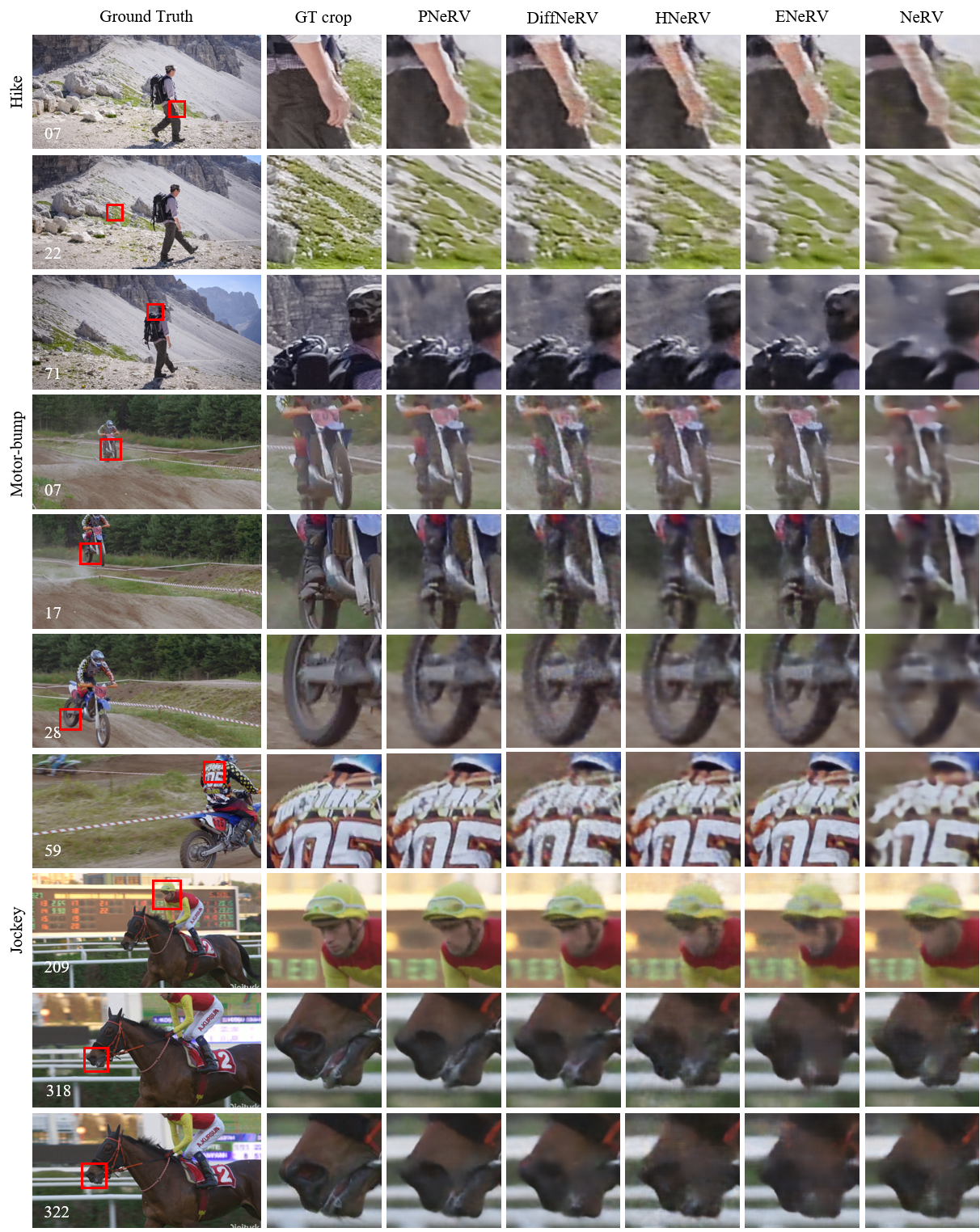
Shown in Fig. D.5, the comparison at different timestamps of the same video indicates some specific common issues of different models. Overlapping and noisy patterns have occurred in the results of DiffNeRV [71] and HNeRV [10], such as the grass and hands in “Hike”. ENeRV [31] and NeRV [9] often result in color deviation and blurring, e.g., backpack in “Hike” and motor in “motor-bump”. PNeRV achieves a balance between preserving details and maintaining semantic consistency. Compared to DiffNeRV, which also uses the difference between frames as input, the latter’s reconstruction of details is unbiased. However, human attention to visual elements under different semantics should be different. Improving the reconstruction results through high-level information is one of PNeRV’s pursuits.

C.5 Discussion on the Failure Cases

As shown in Table 2 , PNeRV fails in the “Dog” which is blurred and mixed with jitter and deformation. Also, the “Soapbox” video, which comprises two clips from entirely different scenes connected by a few frames where the camera rotates through a large angle, poses a challenge. So far, PNeRV has not been able to handle severe temporal inconsistency effectively.

C.6 Video Examples

We provide some video examples from DAVIS as follows. From the video comparison, it can be seen that the reconstructions of NeRV have lost spatial details, and it is difficult for DNeRV to reconstruct videos containing pervasive scattered high-frequency details. Whether there is large motion or high-frequency details in the given videos, PNeRV is more robust in modeling the spatial consistency, leading to better perceptual quality in reconstructions. The links to the examples are presented as follow.
Dance-jump: https://drive.google.com/file/d/18JZq1BCkBJWCkZs-71OB7wI6j_Vma0vP/view?usp=drive_link
Elephant: https://drive.google.com/file/d/1rnPEsEtfA5UADU6BnwEDOPRG9hO9uPuM/view?usp=drive_link
Kite-surf: https://drive.google.com/file/d/1DDGw1zc2iJWcJHdBS4DOnfUQVf2H04Bs/view?usp=drive_link
Parkour: https://drive.google.com/file/d/1jWbJuoc-GCz2N_dXAJSER0PSy7ThrMr-/view?usp=drive_link
Scooter-grey: https://drive.google.com/file/d/1vs22Ru-AwAQuG710qbF72lwdHS1ABy83/view?usp=drive_link

Models	Bmx-B	Camel	Dance-J	Dog	Drift-C	Parkour	Soapbox	Avg.	A.P.G
NeRV [9]	29.42/0.864	24.81/0.781	27.33/0.794	28.17/0.795	36.12/0.969	25.15/0.794	27.68/0.848	28.38/0.835	-
E-NeRV [31]	28.90/0.851	25.85/0.844	29.52/0.855	30.40/0.882	39.26/0.983	25.31/0.845	28.98/0.867	29.75/0.875	-
HNeRV [10]	29.98/0.872	25.94/0.851	29.60/0.850	30.96/0.898	39.27/0.985	26.56/0.851	29.81/0.881	30.30/0.874	-
DiffNeRV [71]	30.58/0.890	27.38/0.887	29.09/0.837	31.32/0.905	40.21/0.987	25.75/0.827	31.47/0.912	30.84/0.892	-
Ablation Study
Bilinear + Concat	24.85/0.783	24.49/0.793	28.32/0.806	26.19/0.723	31.92/0.943	25.09/0.793	29.23/0.872	27.16/0.816	-4.07
Bilinear + GRU	29.86/0.874	25.00/0.811	29.16/0.830	27.11/0.753	32.09/0.945	26.43/0.845	29.10/0.874	28.39/0.847	-2.84
Bilinear + LSTM	26.22/0.792	26.87/0.871	27.85/0.788	26.71/0.741	33.65/0.946	25.82/0.820	29.42/0.881	28.07/0.834	-3.16
Bilinear + BSM	29.97/0.877	27.35/0.881	29.49/0.838	27.14/0.756	34.34/0.968	26.15/0.835	29.14/0.876	29.08/0.862	-2.15
DeConv + Concat	28.06/0.840	24.07/0.774	27.86/0.792	25.16/0.693	34.97/0.961	22.13/0.683	29.33/0.877	27.37/0.803	-3.86
DeConv + GRU	27.52/0.827	28.16/0.900	29.09/0.825	25.76/0.706	37.91/0.980	25.09/0.793	29.54/0.882	29.00/0.845	-2.23
DeConv + LSTM	30.15/0.882	26.49/0.859	28.30/0.805	25.94/0.712	34.91/0.956	26.35/0.842	30.26/0.895	28.91/0.850	-2.32
DeConv + BSM	31.56/0.906	27.18/0.878	29.77/0.847	30.09/0.868	36.03/0.971	26.09/0.831	29.00/0.872	29.96/0.881	-1.27
KFc + Concat	27.51/0.826	25.02/0.816	29.02/0.831	28.80/0.831	36.82/0.974	25.12/0.796	28.53/0.864	28.68/0.848	-2.55
KFc + GRU	31.69/0.910	25.88/0.848	28.32/0.805	28.47/0.813	33.25/0.942	26.68/0.853	30.89/0.903	29.31/0.868	-1.92
KFc + LSTM	29.16/0.862	27.24/0.878	28.90/0.825	29.28/0.842	32.73/0.935	26.62/0.839	29.35/0.879	29.04/0.866	-2.19
KFc + BSM (PNeRV)	31.05/0.896	27.89/0.892	30.45/0.873	31.08/0.898	40.23/0.987	27.08/0.867	30.85/0.902	31.22/0.902	+0

Table C.6: Ablation results on DAVIS subset in PSNR and MS-SSIM, where Avg. is the average PSNR and A.P.G is the average PSNR gap. Every result is reported by corresponding model trained in 300 epoch and 3M size.

	40 $\times$ 80	20 $\times$ 40	10 $\times$ 20
PSNR	31.94	31.33	30.50
SSIM	0.960	0.954	0.947

Table C.7: Embedding size in PNeRV-L.

	1 $\times$ 1	3 $\times$ 3	5 $\times$ 5
PSNR	31.92	31.94	31.90
SSIM	0.960	0.960	0.961

Table C.8: Kernel size in BSM.

	ReLU	Leaky	GeLU	w/o BN
PSNR	31.80	31.86	31.94	31.53
SSIM	0.959	0.961	0.960	0.959

Table C.9: Activation and BN in KFc.

D Additional Ablation Studies

D.1 Ablation Results of Model Structure Details

We ablate the structure details of PNeRV in 3M on “Rollerblade” in $480\times 960$ from DAVIS, given in Tab. C.9, Tab. C.9 and Tab. C.9. The alternation of kernel size or activation has little influence. Encoding more information into embeddings will help the decoder reconstruct better and also increase the overall size.

D.2 Ablation Results of Proposed Modules on DAVIS

To verify the contribution of different modules in PNeRV, we conduct ablation studies on (1) upscaling operators and (2) gated memory mechanisms. We compare KFc with two upscaling layers, Deconv and Bilinear, where “Deconv” is implemented by “nn.ConvTranspose2d” from PyTorch, and “Bilinear” is the combination of bilinear upsampling and Conv2D. KFc achieves better performance due to the global receptive field regardless of what fusion module it is combined with.

Also, to illustrate the importance of adaptive feature fusion and improvement of BSM, we compare BSM with Concat, GRU and LSTM, where “Concat” means directly concatenating two features from different domains together. The ablation results suggest that the adaptive fusion of features from different domains significantly improves performance, and BSM outperforms other memory cells due to the disentangled feature learning. The last row is the final PNeRV and the last column shows PSNR gaps when changing modules in PNeRV.

D.3 Visualization of Feature Maps

To verify the effectiveness of hierarchical information merging via KFc and BSM, we visualize some feature maps in PNeRV-L which was pretrained on “Parkour” as examples. Those feature maps shown in Fig. D.6 are from different channels and layers using the same frame as input. Those in Fig. D.7 are all from the $4$ -th layer but using different frames as input. The feature maps from $4$ -th layer are in $480\times 960$ , and the original frames are in $960\times 1920$ . For each lower layer, the height and width are halved compared to the upper layer. “Before” and “After” refer to the feature maps before and after passing through BSM or after.

Fig. D.6 illustrates how the coarse features are refined by BSM. Different channels respond to distinct spatial patterns of video frames, including factors like color, geometric structure, texture, brightness, motion, and so on. Before being processed by the BSM, the vanilla features are semantically mixed and entangled. However, the BSM is able to decouple these features and distinguish their specific effects, resulting in more refined and distinct outputs.

Additionally, for imperfect feature maps, BSM can add details or balance the focus of the reconstruction across various areas in the frames. These phenomena are commonly observed in the $4$ -th layer, which is responsible for preparing for fine-grained reconstruction, as demonstrated in Figure. D.7. This shows the effectiveness of BSM in enhancing the quality of feature maps and improving the overall reconstruction.

PNeRV: Enhancing Spatial Consistency via Pyramidal Neural Representation for Videos