PLV-IEKF: Consistent Visual-Inertial Odometry using Points, Lines, and Vanishing Points
Abstract
In this paper, we propose an Invariant Extended Kalman Filter (IEKF) based Visual-Inertial Odometry (VIO) using multiple features in man-made environments. Conventional EKF-based VIO usually suffers from system inconsistency and angular drift that naturally occurs in feature-based methods. However, in man-made environments, notable structural regularities, such as lines and vanishing points, offer valuable cues for localization. To exploit these structural features effectively and maintain system consistency, we design a right invariant filter-based VIO scheme incorporating point, line, and vanishing point features. We demonstrate that the conventional additive error definition for point features can also preserve system consistency like the invariant error definition by proving a mathematically equivalent measurement model. And a similar conclusion is established for line features. Additionally, we conduct an invariant filter-based observability analysis proving that vanishing point measurement maintains unobservable directions naturally. Both simulation and real-world tests are conducted to validate our methods’ pose accuracy and consistency. The experimental results validate the competitive performance of our method, highlighting its ability to deliver accurate and consistent pose estimation in man-made environments.
I INTRODUCTION
Accurate pose estimation is a fundamental issue for robot localization, and a range of approaches have been developed in the previous literature which investigates different sensor fusion methods like GNSS [1, 2, 3, 4] and LiDAR [5, 6]. As an attractive candidate, Visual-Inertial Odometry (VIO) has been widely studied for its high accuracy, low cost, and lightweight. Moreover, Extended Kalman Filter (EKF) based VIOs like Multi-State Constraint Kalman Filter (MSCKF) [7] have been favored by many researchers for its great advantage in high computational efficiency.
Conventional MCSKF utilizes point features to constrain the state. However, it may produce a large pose drift in a textureless environment or illumination changing scenes due to the limited number of features in the scene [8]. As an alternative solution, line features may provide additional structural information in challenging environments [9]. Furthermore, vanishing points (VP) in man-made scenarios can make line feature fully observable [10]. Therefore, these structural features can be fully leveraged in VIO to obtain a more accurate pose estimation [11, 12, 13].
Standard EKF frameworks, regardless of whether they use points or lines, have been proven to be inconsistent due to spurious information along the unobservable direction [12]. To address this issue, various algorithms have been proposed. In recent years, the Invariant EKF (IEKF) has been successfully applied in robotic localization, particularly in filter-based VIO [14, 15, 16, 17]. The IEKF model defines an alternative nonlinear error for estimated poses and landmarks, automatically ensuring the appropriate dimension of the unobservable subspace [18]. However, in the case of MSCKF, landmarks are not included in the state. This leads to two different error definitions for landmarks: the nonlinear error definition following IEKF and the additive error definition following the conventional MSCKF. The relationship between these two definitions and their impact on filter consistency is our motivation to investigate.
Our main contributions are summarized as follows:
-
•
We present a right invariant filter-based VIO leveraging points, lines, and vanishing points, which improves both the pose consistency and accuracy.
-
•
In the filter design, we prove an equivalent measurement model for point features, demonstrating that these features do not change the filter consistency even in the conventional error representation when they are decoupled from the state vector. And a similar conclusion can be given for line features.
-
•
An observability analysis is given to demonstrate that our method maintains the system’s unobservable subspace naturally and enhances the observability of line features.
II RELATED WORKS
II-A IEKF Applications for VIO
IEKF [19] is proposed to address the filter inconsistency problem, which has been widely researched in a range of literature [18, 20, 21, 22, 23, 24, 25]. The IEKF model has been further applied to MSCKF [12, 14, 26] and UKF [15]. Previous works [14], [27] have coupled the landmark uncertainty with the camera pose, while other works adopt the simple addictive error [26]. Though both strategies can maintain the consistency, the relationship between two kinds of error definition has not been investigated.
II-B Point-Line-VIO
A couple of works have combined point and line features. Among optimization-based methods, [9] jointly minimizes the IMU pre-integration constraints together with the point and line re-projection errors. [28] further modifies the LSD [29] algorithm to have a better real-time performance based on [9]. By utilizing the structural regularity, Lee et al. introduce parallel lines’ constraints into point-line-based VIO and present a novel structural line triangulation method making full use of the prior information [13]. Among filter-based methods, the issue of point-line VIO inconsistency is addressed and improved by observability-constrained techniques [30] and the IEKF framework [12]. [31] extends a new line parameterization for processing the line observations in a rolling shutter camera setting. Zheng et al. present Trifo-VIO which incorporates point and line feature measurements and formulate loop closure as EKF updates [32]. [33] investigates two line triangulation methods and reveals three degenerate motions which cause triangulation failures.
II-C Vanishing Point aided SLAM/VIO
In man-made environments, geometric information like vanishing points can also boost the robustness of VIO and Simultaneous Localization and Mapping (SLAM) [34, 35, 36, 37]. Zhang et al. provide a solution to the loop closure problem leveraging vanishing points in line-based SLAM [38]. [39] proposes an efficient line classification method for detecting vanishing points and keeps the vanishing points in the VIO state for a long tracking. Xu et al. design a point-line-based VIO system where vanishing points are used to recognize and classify structural lines [40]. In [10], the vanishing point cost function is added into the optimization-based VIO without the constraints like the Manhattan world assumption [41]. However, these works have not focused on consistency about vanishing point measurements.
III PRELIMINARY KNOWLEDGE
III-A IEKF Model
In the visual-inertial navigation system, the defined state is given by:
| (1) |
where is the landmark. Unlike the conventional error in standard EKF, the right invariant filter employs a new uncertainty representation:
| (2) | ||||
where is the left Jacobian for Lie group, and is the state error vector. Note that apart from robot velocity and position, the landmark’s uncertainty is also coupled with the rotation state. This nonlinear error allows the system to obtain a better performance on consistency.
III-B Line Representation
There exist many representation models for a 3D line, and two representations are focused on in our paper. One is the conventional Plucker coordinate , where is the normal vector of the plane determined by the line and the coordinate origin, and is the line direction vector [9]. However, this representation has redundant parameters since the degrees of freedom for a line should be four, so the minimal representation is more suitable in line optimization:
| (3) | ||||
where denotes the skew symmetric matrix.
IV FILTER DESCRIPTION
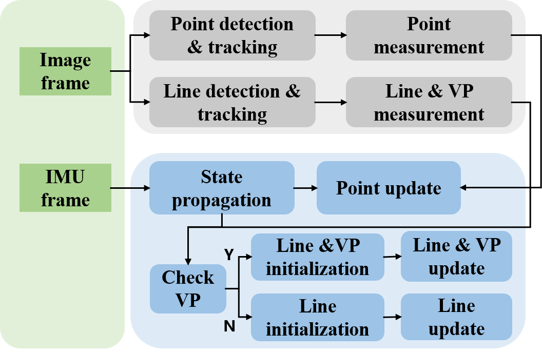
In the following sections, we denote the estimated state as , and the error state as . We build our system based on IEKF framework, as shown in Fig. 1. Specifically, we define the system state as:
| (4) | ||||
| (5) | ||||
| (6) |
where is the sliding window length. and represents the IMU state and camera pose respectively, is the rotation from the IMU frame to the global frame, and are the global velocity and position of IMU, respectively. and are the gyroscope and acceleromter biases, respectively. Note that we do not incorporate landmarks in , which is different from the conventional IEKF model in (1). In other words, landmarks are decoupled from the state.
IV-A IMU Kinematic Model
The IMU continuous kinematic model is given by:
| (7) | ||||
where and are the angular velocity and linear acceleration velocity, respectively. and are Gaussian noises. After linearization, the following propagation equation is obtained:
| (8) |
where is the process noise. is the continuous state transition matrix and is the input noise Jacobian.
IV-B Point Measurement Model
When the position of the point feature is initialized, the normalized coordinate of the feature point is obtained:
| (9) |
where is the projection function. The corresponding error vector of is denoted as . Therefore, the linearized measurement model can be obtained as below:
| (10) |
where Jacobians and are given by (25) in Appendix. Genrally, follows an invariant error definition like (2):
| (11) |
where is the orientation error for , and is the camera pose that captures the landmark first. However, a proposition is given to reveal the equivalent relationship between the right invariant form and the conventional error form, i.e. .
Given the same estimated landmark, the measurement model for points is equivalent for the invariant error and additive error.
Proof: See Appendix.
Remark: The equivalent measurement model indicates the same consistency property. However, the additive error definition is more convenient to implement.
IV-C Line Measurement Model
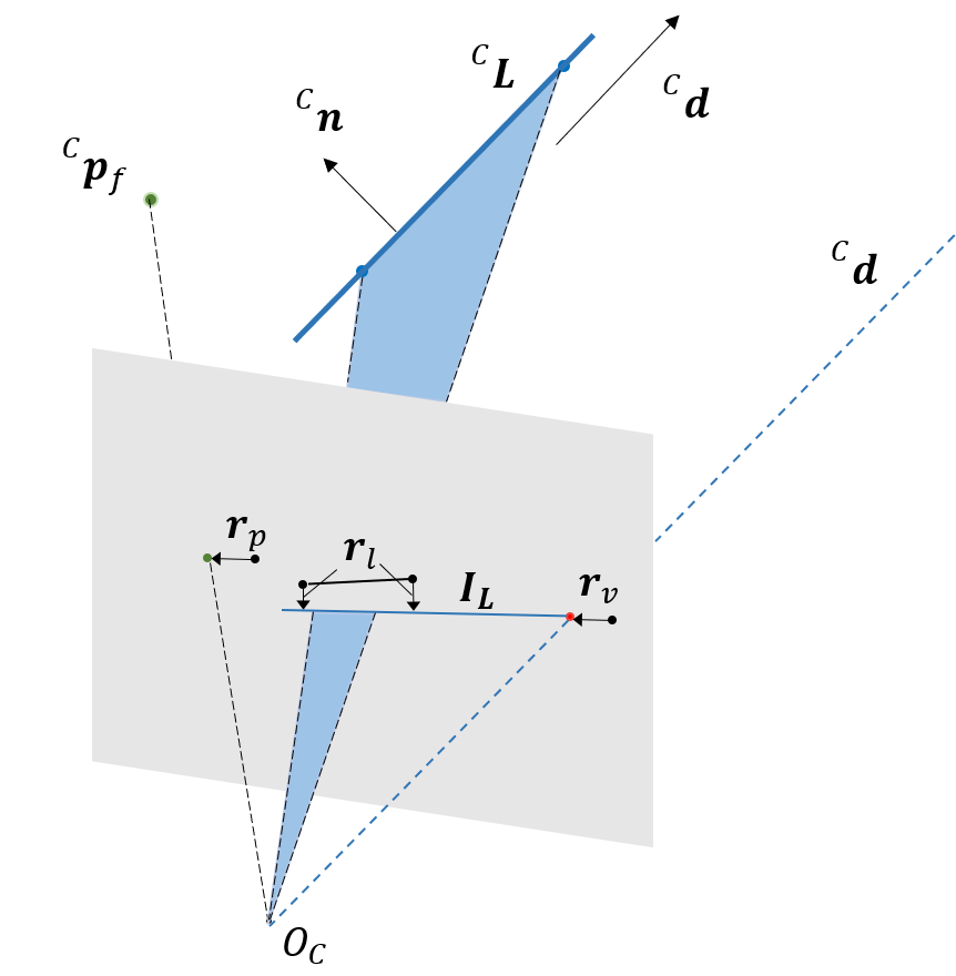
As shown in Fig. 2, represents the projection of a straight line on the normalized image plane, so the error term is defined as the distance between the endpoints on the line in an image and the estimated 2D line:
| (12) |
where is the re-projected line on the normalized plane, and are the endpoint measurements of the line on the normalized plane.
The line error for the orthonormal representation is classified into globally-defined error and locally-defined error as below:
| (13) | |||
Thus, a conclusion on these two error forms can be given:
Given the same estimated line, the measurement models for lines are equivalent for the globally-defined error and locally-defined error.
Proof: The proof is similar to that of 1.
Remark: Conventional line-based VIO usually chooses the locally-defined error [9] while IEKF-based VIO [12] may choose the global one. Since the line feature is not incorporated in the state variables, both errors are acceptable in the algorithm implementation.
Therefore, the linearized measurement model following a globally-defined error is given by:
| (14) | ||||
where is the Jacobian of line projection, .
IV-D Vanishing Point Measurement Model
In the man-made environment, lines can be classified into structural lines with VP measurements and non-structural lines [10]. For a structural line, when its corresponding vanishing point is calculated, a VP measurement residual is obtained:
| (15) |
where and represent the vanishing point residual and the vanishing point observation, respectively. is the line direction vector in the camera frame, which is orthogonal to the normal vector which is used as the line measurement. In this sense, VP measurement is complementary to line measurement and fully exploits the line geometric information. The Jacobian with respect to the vanishing point is computed as follows:
| (16) | ||||
where the Jacobian items are similar to those in (14).
V FEATURE INITIALIZATION
V-A Line & VP Detection
When a new frame comes, line segments are detected by the LSD detector. For each line, the descriptor LBD is calculated for line tracking. Some outlier rejection strategies are employed such as the limited distance between the endpoints of matched lines and the limited angle difference between the line directions. As for VP detection, we use the efficient and robust two-line based VP detection algorithm [42], and the observed lines with the detected VPs will be considered as the structural lines and used in the aforementioned line measurement model and VP measurement model.
V-B Line & VP Estimation
The strategy of line estimation is similar to that of point estimation in MSCKF. When a non-structural line is no longer tracked by the current camera frame, it will be triangulated by the dual Plucker matrix method [9]. Then we optimize it by the following cost function:
| (17) |
where are the sets of non-structural line measurements in the sliding window, is the -th line measurement. After the structural line is triangulated, we add a VP cost item for a better estimation:
| (18) |
where are the sets of structural line measurement, is the -th vanishing point measurement.
VI OBSERVABILITY ANALYSIS
In this section, we perform the observability analysis of our proposed method based on the EKF model which has the same observability property as MSCKF. The observability matrix for EKF in the period [] is defined as follows:
| (19) |
where is the measurement Jacobian, is the state transition matrix from to . Since previous literature has demonstrated that point-line based IEKF can improve the consistency without artificial remedies [12], we focus on the observability of the vanishing point. At time step , the state vector is considered to contain only one line feature with the line and VP measurement. The observability matrix at can be written as:
| (20) |
The null space for has been derived in [12], indicating that the unobservable subspace does not degenerate. And the second part can be derived as:
| (21) | ||||
There are at least eleven directions lying in the unobservable subspace with the null space matrix:
| (22) |
It is observed that the left nine columns of are independent of the estimated state. Therefore, the IEKF model with line features can remain in the ideal unobservable subspace naturally. Meanwhile, there exist at least two unobservable directions for :
| (23) |
where is the null space matrix of , and represents the null space regarding the line parameter. It can be verified that which means the line is fully observable with VP measurements.
VII EVALUATION
To validate the effectiveness of our proposed approach, we conduct the simulation and real-world test. In the real-world test, we compare our algorithm with some state-of-the-art VIO algorithms. Our experiments are conducted on a laptop with Intel(R) Core(TM) i7-10710U [email protected] and 16G RAM.
VII-A Simulation
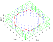
In the simulation test, we assume that a car equipped with a 100Hz IMU and a 10Hz camera loops ten times along a circle with a radius of 6m. A total of 200 points and 140 lines are scattered around the real trajectory, as shown in Fig. 3(a). The points are generated along the inside cylinder wall with a radius of 5 meters and outside cylinder walls with a radius of 7 meters. And the lines are generated along a square wall with a length of 14 meters. The camera captures landmarks in the field of view of the camera within a range of 20 meters. We generate sensor measurements with noise according to the trajectory and landmarks. The initial noise matrix is set as , and all the feature measurement noise is set as 1 pixel.
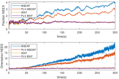
Four algorithms are compared in the simulation: standard point based MSCKF (MSCKF), standard point based IEKF, point-line-VP based MSCKF (PLV-MSCKF), and point-line-VP based IEKF (PLV-IEKF). The sliding window size is set as 20 and we only use the landmarks that are captured more than 5 times by the camera for robust estimation. The pose accuracy indicator Root Mean Squared Error (RMSE) and the consistency indicator Averaged Normalized Estimation Error Squared (ANEES) are reported in Fig. 3(b) and (c). It is evident that NEES of IEKF and PLV-IEKF is closer to the ideal NEES (one) than that of MSCKF family, indicating better consistency. Meanwhile, PLV-IEKF achieves a better pose estimation than IEKF with additional line and VP measurements.
| Sequence | Algorithm | ||||||
| 8 | |||||||
| MSCKF | PLV-MSCKF | IEKF | PL-IEKF | VINS-Mono | PL-VINS | PLV-IEKF | |
| MH_01_easy | 0.265 | 0.229 | 0.257 | 0.216 | 0.182 | 0.174 | |
| MH_02_easy | 0.295 | 0.237 | 0.250 | 0.229 | 0.232 | 0.208 | |
| MH_03_medium | 0.443 | 0.413 | 0.298 | 0.222 | 0.269 | 0.267 | |
| MH_04_difficult | 0.605 | 0.346 | 0.403 | 0.460 | 0.439 | 0.409 | |
| MH_05_difficult | 0.404 | 0.285 | 0.294 | 0.325 | 0.300 | 0.328 | |
| V1_01_easy | 0.105 | 0.098 | 0.079 | 0.082 | 0.087 | 0.073 | |
| V1_02_medium | 0.144 | 0.160 | 0.140 | 0.164 | 0.171 | 0.182 | |
| V1_03_difficult | 0.376 | 0.308 | 0.331 | 0.272 | 0.250 | 0.249 | |
| V2_01_easy | 0.349 | 0.154 | 0.242 | 0.187 | 0.165 | 0.141 | |
| V2_02_medium | 0.253 | 0.240 | 0.245 | 0.268 | 0.209 | 0.224 | |
| * Bold and underline represent best and second best in each sequence, respectively. | |||||||
VII-B Real-world Test
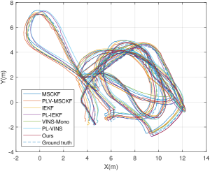
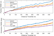
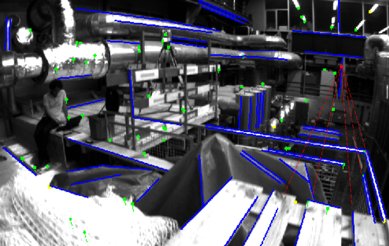
To validate the effect of our proposed method, we conduct a real-world experiment on EuRoC Dataset [43], which exhibits varying levels of motion blur and textureless regions [33]. V2_03_difficult sequence is not chosen due to a number of missing camera frames which affect the feature tracking. We compare our algorithm with other state-of-the-art algorithms such as MSCKF [44], IEKF [27], VINS-Mono [45] and PL-VINS [28]. PLV-MSCKF and point-line based invariant IEKF (PL-IEKF) are also implemented for a detailed comparison. For all of the algorithms, we extract no less than 100 point features and 30 line features for robust estimation and disable loop detection for a fair comparison. The sliding window size for these filter-based VIO is set as 20. An example of tracked features in MH_03_medium is shown in Fig. 4. RMSE results are reported in Table I, and the trajectory sample is shown in Fig. 5. It is evident that in most cases using lines and vanishing points can achieve a better pose accuracy, and PLV-IEKF has a better performance than PLV-MSCKF because of better consistency.
It is also observed in Table I that PLV-IEKF performs better in Machine Hall (MH) sequences than PL-IEKF since there exist more structural features in the environment, where vanishing point measurements can improve the line estimation, even in challenging sequences like MH_04_difficult sequence with illumination changing and textureless scenarios.
| Algorithm | MSCKF | PLV-MSCKF | IEKF | PL-IEKF | VINS-Mono | PL-VINS | PLV-IEKF |
| Time cost (ms) | 5.21 | 5.578 | 5.33 | 5.43 | 37.9 | 60.06 | 5.65 |
Table II shows the backend processing time on MH_01_easy sequence for different algorithms, among which the proposed PLV-IEKF requires slightly more time than other filter-based point-based and point-line-based methods, but much less time than VINS-Mono and PL-VINS. It demonstrates that PL-IEKF can achieve competitive and higher time efficiency compared with optimization-based methods.
VIII CONCLUSIONS
In this paper, we propose an invariant Visual-Inertial Odometry (VIO) leveraging points, lines, and vanishing point features in man-made environments. Three feature measurement models are obtained in our framework, and two equivalent measurement models of points and lines are proven in our filter design. The observability matrix regarding vanishing points is derived to demonstrate that the EKF model with line features can guarantee the ideal unobservable subspace. Simulation tests and real-world experiments validate our algorithm’s consistency and competitive accuracy compared with other state-of-the-art algorithms. In the future, we will refine the line and VP estimation to achieve an accurate and efficient mapping.
APPENDIX
VIII-A Proof of Proposition 1
To prove Proposition 1, we assume that only one point-type landmark in the current sliding window is observed by camera poses. When the landmark error is additive, the Jacobian for VIO state is given by:
| (24) | ||||
where , is the Jacobian for the -th camera pose. On the other hand, the Jacobian regarding an invariant form is calculated as follows:
| (25) | ||||
Note that the Jacobians with respect to the landmark for both forms are the same:
| (26) |
which shares the same left null space matrix . We calculate the difference between the final Jacobians:
| (27) | ||||
Therefore the final Jacobians are equivalent, so is the final projected measurement noise .
References
- [1] S. Cao, X. Lu, and S. Shen, “GVINS: Tightly coupled gnss-visual-inertial fusion for smooth and consistent state estimation,” IEEE Transactions on Robotics, vol. 38, no. 4, pp. 2004–2021, 2022.
- [2] W. Lee, K. Eckenhoff, P. Geneva, and G. Huang, “Intermittent gps-aided vio: Online initialization and calibration,” in 2020 IEEE International Conference on Robotics and Automation (ICRA). IEEE, 2020, pp. 5724–5731.
- [3] T. Li, L. Pei, Y. Xiang, W. Yu, and T.-K. Truong, “P3-VINS: Tightly-coupled ppp/ins/visual SLAM based on optimization approach,” IEEE Robotics and Automation Letters, vol. 7, no. 3, pp. 7021–7027, 2022.
- [4] T. Hua, L. Pei, T. Li, J. Yin, G. Liu, and W. Yu, “M2C-GVIO: motion manifold constraint aided gnss-visual-inertial odometry for ground vehicles,” Satellite Navigation, vol. 4, no. 1, pp. 1–15, 2023.
- [5] J. Zhang and S. Singh, “LOAM: Lidar odometry and mapping in real-time.” in Robotics: Science and systems, vol. 2, no. 9. Berkeley, CA, 2014, pp. 1–9.
- [6] T. Li, L. Pei, Y. Xiang, X. Zuo, W. Yu, and T.-K. Truong, “P3-LINS: Tightly coupled ppp-gnss/ins/lidar navigation system with effective initialization,” IEEE Transactions on Instrumentation and Measurement, vol. 72, pp. 1–13, 2023.
- [7] A. I. Mourikis and S. I. Roumeliotis, “A multi-state constraint Kalman filter for vision-aided inertial navigation,” in 2007 IEEE International Conference on Robotics and Automation, 2007, pp. 3565–3572.
- [8] H. Zhou, D. Zou, L. Pei, R. Ying, P. Liu, and W. Yu, “StructSLAM: Visual SLAM with building structure lines,” IEEE Transactions on Vehicular Technology, vol. 64, no. 4, pp. 1364–1375, 2015.
- [9] Y. He, J. Zhao, Y. Guo, W. He, and K. Yuan, “PL-VIO: Tightly-coupled monocular visual–inertial odometry using point and line features,” Sensors, vol. 18, no. 4, p. 1159, 2018.
- [10] H. Lim, J. Jeon, and H. Myung, “UV-SLAM: Unconstrained line-based SLAM using vanishing points for structural mapping,” IEEE Robotics and Automation Letters, vol. 7, no. 2, pp. 1518–1525, 2022.
- [11] D. Zou, Y. Wu, L. Pei, H. Ling, and W. Yu, “Structvio: Visual-inertial odometry with structural regularity of man-made environments,” IEEE Transactions on Robotics, vol. 35, no. 4, pp. 999–1013, 2019.
- [12] S. Heo, J. H. Jung, and C. G. Park, “Consistent ekf-based visual-inertial navigation using points and lines,” IEEE Sensors Journal, vol. 18, no. 18, pp. 7638–7649, 2018.
- [13] J. Lee and S.-Y. Park, “Plf-vins: Real-time monocular visual-inertial SLAM with point-line fusion and parallel-line fusion,” IEEE Robotics and Automation Letters, vol. 6, no. 4, pp. 7033–7040, 2021.
- [14] K. Wu, T. Zhang, D. Su, S. Huang, and G. Dissanayake, “An invariant-EKF vins algorithm for improving consistency,” in 2017 IEEE/RSJ international conference on intelligent robots and systems (IROS). IEEE, 2017, pp. 1578–1585.
- [15] M. Brossard, S. Bonnabel, and A. Barrau, “Invariant Kalman filtering for visual inertial SLAM,” in 2018 21st International Conference on Information Fusion (FUSION). IEEE, 2018, pp. 2021–2028.
- [16] Z. Zhang, Y. Song, S. Huang, R. Xiong, and Y. Wang, “Toward consistent and efficient map-based visual-inertial localization: Theory framework and filter design,” IEEE Transactions on Robotics, 2023.
- [17] J. H. Jung, Y. Choe, and C. G. Park, “Photometric visual-inertial navigation with uncertainty-aware ensembles,” IEEE Transactions on Robotics, vol. 38, no. 4, pp. 2039–2052, 2022.
- [18] A. Barrau and S. Bonnabel, “An EKF-SLAM algorithm with consistency properties,” arXiv preprint arXiv:1510.06263, 2015.
- [19] S. Bonnabel, “Left-invariant extended Kalman filter and attitude estimation,” in 2007 46th IEEE Conference on Decision and Control. IEEE, 2007, pp. 1027–1032.
- [20] T. Bailey, J. Nieto, J. Guivant, M. Stevens, and E. Nebot, “Consistency of the EKF-SLAM algorithm,” in 2006 IEEE/RSJ International Conference on Intelligent Robots and Systems. IEEE, 2006, pp. 3562–3568.
- [21] S. Huang and G. Dissanayake, “Convergence and consistency analysis for extended Kalman filter based SLAM,” IEEE Transactions on robotics, vol. 23, no. 5, pp. 1036–1049, 2007.
- [22] G. P. Huang, A. I. Mourikis, and S. I. Roumeliotis, “Analysis and improvement of the consistency of extended Kalman filter based SLAM,” in 2008 IEEE International Conference on Robotics and Automation. IEEE, 2008, pp. 473–479.
- [23] M. Li and A. I. Mourikis, “High-precision, consistent EKF-based visual-inertial odometry,” The International Journal of Robotics Research, vol. 32, no. 6, pp. 690–711, 2013.
- [24] G. P. Huang, A. I. Mourikis, and S. I. Roumeliotis, “Observability-based rules for designing consistent EKF SLAM estimators,” The International Journal of Robotics Research, vol. 29, no. 5, pp. 502–528, 2010.
- [25] T. Hua, T. Li, and L. Pei, “PIEKF-VIWO: Visual-inertial-wheel odometry using partial invariant extended Kalman filter,” arXiv preprint arXiv:2303.07668, 2023.
- [26] X. Li, H. Jiang, X. Chen, H. Kong, and J. Wu, “Closed-form error propagation on SE group for invariant EKF with applications to vins,” IEEE Robotics and Automation Letters, vol. 7, no. 4, pp. 10 705–10 712, 2022.
- [27] M. Brossard, S. Bonnabel, and A. Barrau, “Unscented Kalman filter on lie groups for visual inertial odometry,” in 2018 IEEE/RSJ International Conference on Intelligent Robots and Systems (IROS). IEEE, 2018, pp. 649–655.
- [28] Q. Fu, J. Wang, H. Yu, I. Ali, F. Guo, Y. He, and H. Zhang, “Pl-vins: Real-time monocular visual-inertial SLAM with point and line features,” arXiv preprint arXiv:2009.07462, 2020.
- [29] R. G. Von Gioi, J. Jakubowicz, J.-M. Morel, and G. Randall, “Lsd: A fast line segment detector with a false detection control,” IEEE transactions on pattern analysis and machine intelligence, vol. 32, no. 4, pp. 722–732, 2008.
- [30] D. G. Kottas and S. I. Roumeliotis, “Efficient and consistent vision-aided inertial navigation using line observations,” in 2013 IEEE International Conference on Robotics and Automation. IEEE, 2013, pp. 1540–1547.
- [31] H. Yu and A. I. Mourikis, “Vision-aided inertial navigation with line features and a rolling-shutter camera,” in 2015 IEEE/RSJ International Conference on Intelligent Robots and Systems (IROS). IEEE, 2015, pp. 892–899.
- [32] F. Zheng, G. Tsai, Z. Zhang, S. Liu, C.-C. Chu, and H. Hu, “Trifo-VIO: Robust and efficient stereo visual inertial odometry using points and lines,” in 2018 IEEE/RSJ International Conference on Intelligent Robots and Systems (IROS). IEEE, 2018, pp. 3686–3693.
- [33] Y. Yang, P. Geneva, K. Eckenhoff, and G. Huang, “Visual-inertial odometry with point and line features,” in 2019 IEEE/RSJ International Conference on Intelligent Robots and Systems (IROS). IEEE, 2019, pp. 2447–2454.
- [34] A. Pumarola, A. Vakhitov, A. Agudo, A. Sanfeliu, and F. Moreno-Noguer, “PL-SLAM: Real-time monocular visual SLAM with points and lines,” in 2017 IEEE international conference on robotics and automation (ICRA). IEEE, 2017, pp. 4503–4508.
- [35] R. Gomez-Ojeda, F.-A. Moreno, D. Zuniga-Noël, D. Scaramuzza, and J. Gonzalez-Jimenez, “PL-SLAM: A stereo SLAM system through the combination of points and line segments,” IEEE Transactions on Robotics, vol. 35, no. 3, pp. 734–746, 2019.
- [36] H. Li, J. Yao, J.-C. Bazin, X. Lu, Y. Xing, and K. Liu, “A monocular SLAM system leveraging structural regularity in manhattan world,” in 2018 IEEE International Conference on Robotics and Automation (ICRA). IEEE, 2018, pp. 2518–2525.
- [37] A. Georgis, P. Mermigkas, and P. Maragos, “VP-SLAM: A monocular real-time visual SLAM with points, lines and vanishing points,” arXiv preprint arXiv:2210.12756, 2022.
- [38] G. Zhang, D. H. Kang, and I. H. Suh, “Loop closure through vanishing points in a line-based monocular SLAM,” in 2012 IEEE International Conference on Robotics and Automation. IEEE, 2012, pp. 4565–4570.
- [39] F. Camposeco and M. Pollefeys, “Using vanishing points to improve visual-inertial odometry,” in 2015 IEEE international conference on robotics and automation (ICRA). IEEE, 2015, pp. 5219–5225.
- [40] B. Xu, P. Wang, Y. He, Y. Chen, Y. Chen, and M. Zhou, “Leveraging structural information to improve point line visual-inertial odometry,” IEEE Robotics and Automation Letters, vol. 7, no. 2, pp. 3483–3490, 2022.
- [41] J. Coughlan and A. L. Yuille, “The manhattan world assumption: Regularities in scene statistics which enable bayesian inference,” Advances in Neural Information Processing Systems, vol. 13, 2000.
- [42] X. Lu, J. Yaoy, H. Li, Y. Liu, and X. Zhang, “2-line exhaustive searching for real-time vanishing point estimation in manhattan world,” in 2017 IEEE Winter Conference on Applications of Computer Vision (WACV). IEEE, 2017, pp. 345–353.
- [43] M. Burri, J. Nikolic, P. Gohl, T. Schneider, J. Rehder, S. Omari, M. W. Achtelik, and R. Siegwart, “The EuRoC micro aerial vehicle datasets,” The International Journal of Robotics Research, vol. 35, no. 10, pp. 1157–1163, 2016.
- [44] K. Sun, K. Mohta, B. Pfrommer, M. Watterson, S. Liu, Y. Mulgaonkar, C. J. Taylor, and V. Kumar, “Robust stereo visual inertial odometry for fast autonomous flight,” IEEE Robotics and Automation Letters, vol. 3, no. 2, pp. 965–972, 2018.
- [45] T. Qin, P. Li, and S. Shen, “VINS-Mono: A robust and versatile monocular visual-inertial state estimator,” IEEE Transactions on Robotics, vol. 34, no. 4, pp. 1004–1020, 2018.