Plug-In Inversion: Model-Agnostic Inversion for Vision with Data Augmentations
Abstract
Existing techniques for model inversion typically rely on hard-to-tune regularizers, such as total variation or feature regularization, which must be individually calibrated for each network in order to produce adequate images. In this work, we introduce Plug-In Inversion, which relies on a simple set of augmentations and does not require excessive hyper-parameter tuning. Under our proposed augmentation-based scheme, the same set of augmentation hyper-parameters can be used for inverting a wide range of image classification models, regardless of input dimensions or the architecture. We illustrate the practicality of our approach by inverting Vision Transformers (ViTs) and Multi-Layer Perceptrons (MLPs) trained on the ImageNet dataset, tasks which to the best of our knowledge have not been successfully accomplished by any previous works.
1 Introduction
Model inversion is an important tool for visualizing and interpreting behaviors inside neural architectures, understanding what models have learned, and explaining model behaviors. In general, model inversion seeks inputs that either activate a feature in the network (feature visualization) or yield a high output response for a particular class (class inversion) (Olah et al., 2017). Model inversion and visualization has been a cornerstone of conceptual studies that reveal how networks decompose images into semantic information (Zeiler & Fergus, 2014; Dosovitskiy & Brox, 2016). Over time, inversion methods have shifted from solving conceptual problems to solving practical ones. Saliency maps, for example, are image-specific model visualizations that reveal the inputs that most strong influence a model’s decisions (Simonyan et al., 2014).
Recent advances in network architecture pose major challenges for existing model inversion schemes. Convolutional Neural Networks (CNN) have long been the de-facto approach for computer vision tasks, and are the focus of nearly all research in the model inversion field. Recently, other architectures have emerged that achieve results competitive with CNNs. These include Vision Transformers (ViTs; Dosovitskiy et al., 2021), which are based on self-attention layers, and MLP-Mixer (Tolstikhin et al., 2021) and ResMLP (Touvron et al., 2021a), which are based on Multi Layer Perceptron layers. Unfortunately, most existing model inversion methods either cannot be applied to these architectures, or are known to fail. For example, the feature regularizer used in DeepInversion (Yin et al., 2020) cannot be applied to ViTs or MLP-based models because they do not include Batch Normalization layers (Ioffe & Szegedy, 2015).
In this work, we focus on class inversion, the goal of which is to find interpretable images that maximize the score a classification model assigns to a chosen label without knowledge about the model’s training data. Class inversion has been used for a variety of tasks including model interpretation (Mordvintsev et al., 2015), image synthesis (Santurkar et al., 2019), and data-free knowledge transfer (Yin et al., 2020). However, current inversion methods have several key drawbacks. The quality of generated images is often highly sensitive to the weights assigned to regularization terms, so these hyper-parameters need to be carefully calibrated for each individual network. In addition, methods requiring batch norm parameters are not applicable to emerging architectures.
To overcome these limitations, we present Plug-In Inversion (PII), an augmentation-based approach to class inversion. PII does not require any explicit regularization, which eliminates the need to tune regularizer-specific hyper-parameters for each model or image instance. We show that PII is able to invert CNNs, ViTs, and MLP networks using the same architecture-agnostic method, and with the same architecture-agnostic hyper-parameters.
We summarize our contributions as follows:
-
We provide a detailed analysis of various augmentations and how they affect the quality of images produced via class inversion.
-
We introduce Plug-In Inversion (PII), a new class inversion technique based on these augmentations, and compare it to existing techniques.
-
We apply PII to dozens of different pre-trained models of varying architecture, justifying the claim that it can be ‘plugged in’ to most networks without modification.
-
In particular, we show that PII succeeds in inverting ViTs and large MLP-based architectures, which to our knowledge has not previously been accomplished.
-
Finally, we explore the potential for combining PII with prior methods.
2 Background
2.1 Class inversion
In the basic procedure for class inversion, we begin with a pre-trained model and chosen target class . We randomly initialize (and optionally pre-process) an image in the input space of . We then perform gradient descent to solve the optimization problem for a chosen objective function to produce a class image . For very shallow networks and small datasets, letting be cross-entropy or even the negative confidence assigned to the true class can produce recognizable images with minimal pre-processing (Fredrikson et al., 2015). Modern deep neural networks, however, cannot be inverted as easily.
2.2 Regularization
Most prior work on class inversion for deep networks has focused on carefully designing the objective function to produce quality images. This entails combining a divergence term (e.g. cross-entropy) with one or more regularization terms (image priors) meant to guide the optimization towards an image with ‘natural’ characteristics. DeepDream (Mordvintsev et al., 2015), following work on feature inversion (Mahendran & Vedaldi, 2015), uses two such terms: , which penalizes the magnitude of the image vector, and total variation, defined as , which penalizes sharp changes over small distances.
DeepInversion (Yin et al., 2020) uses both of these regularizers, along with the feature regularizer , where are the batch mean and variance of the features output by the -th convolutional layer, and are corresponding Batch Normalization statistics stored in the model (Ioffe & Szegedy, 2015). Naturally, this method is only applicable to models that use Batch Normalization, which leaves out ViTs, MLPs, and even some CNNs. Furthermore, the optimal weights for each regularizer in the objective function vary wildly depending on architecture and training set, which presents a barrier to easily applying such methods to a wide array of networks.
| w/ Centering | w/o Centering | ||||||||
| Init | Step 1 | Step 2 | Step 3 | Step 4 | Step 5 | Step 6 | Step 7 | Final | Final |
 |
 |
 |
 |
 |
 |
 |
 |
 |
|
| w/ Zoom | w/o Zoom | ||||||||
| Init | Step 1 | Step 2 | Step 3 | Step 4 | Step 5 | Step 6 | Step 7 | Final | Final |
|
|
|
|
|
|
|
|
|
|
2.3 Architectures for vision
We now present a brief overview of the three basic types of vision architectures that we will consider.
Convolutional Neural Networks (CNNs) have long been the standard in deep learning for computer vision (LeCun et al., 1989; Krizhevsky et al., 2012). Convolutional layers encourage a model to learn properties desirable for vision tasks, such as translation invariance. Numerous CNN models exist, mainly differing in the number, size, and arrangement of convolutional blocks and whether they include residual connections, Batch Normalization, or other modifications (He et al., 2016; Zagoruyko & Komodakis, 2016; Simonyan & Zisserman, 2014).
Dosovitskiy et al. (2021) recently introduced Vision Transformers (ViTs), adapting the Transformer architectures commonly used in NLP (Vaswani et al., 2017). ViTs break input images into patches, combine them with positional embeddings, and use these as input tokens to self-attention modules. Some proposed variants require less training data (Touvron et al., 2021c), have convolutional inductive biases (d’Ascoli et al., 2021), or make other modifications to the attention modules (Chu et al., 2021; Liu et al., 2021b; Xu et al., 2021).
Subsequently, a number of authors have proposed vision models which are based solely on Multi-Layer Perceptrons (MLPs), using insights from ViTs (Tolstikhin et al., 2021; Touvron et al., 2021a; Liu et al., 2021a). Generally, these models use patch embeddings similar to ViTs and alternate channel-wise and patch-wise linear embeddings, along with non-linearities and normalization.
We emphasize that as the latter two architecture types are recent developments, our work is the first to study them in the context of model inversion.
3 Plug-In Inversion
Prior work on class inversion uses augmentations like jitter, which randomly shifts an image horizontally and vertically, and horizontal flips to improve the quality of inverted images (Mordvintsev et al., 2015; Yin et al., 2020). The hypothesis behind their use is that different views of the same image should result in similar scores for the target class. These augmentations are applied to the input before feeding it to the network, and different augmentations are used for each gradient step used to reconstruct . In this section, we explore additional augmentations that benefit inversion before describing how we combine them to form the PII algorithm.
| w/ CS |

|

|
|

|

|

|
| w/o CS |
|
|
|
|
|
|

|

|

|

|

|

|

|
As robust models are typically easier to invert than naturally trained models (Santurkar et al., 2019; Mejia et al., 2019), we use a robust ResNet-50 (He et al., 2016) model trained on the ImageNet (Deng et al., 2009) dataset throughout this section as a toy example to examine how different augmentations impact inversion. Note, we perform the demonstrations in this section under slightly different conditions and with different models than those ultimately used for PII in order to highlight the effects of the augmentations as clearly as possible. The reader may find thorough experimental details in the appendix, section C.
3.1 Restricting Search Space
In this section, we consider two augmentations to improve the spatial qualities of inverted images: Centering and Zoom. These are designed based on our hypothesis that restricting the input optimization space encourages better placement of recognizable features. Both methods start with small input patches, and each gradually increases this space in different ways to reach the intended input size. In doing so, they force the inversion algorithm to place important semantic content in the center of the image.
Centering
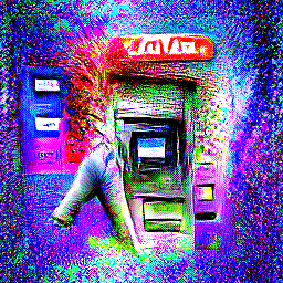
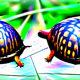
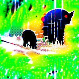
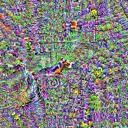
Let be the input image being optimized. At first, we only optimize a patch at the center of . After a fixed number of iterations, we increase the patch size outward by padding with random noise, repeating this until the patch reaches the full input size. Figure 1 shows the state of the image prior at each stage of this process, as well as an image produced without centering. Without centering, the shift invariance of the networks allows most semantic content to scatter to the image edges. With centering, results remain coherent.
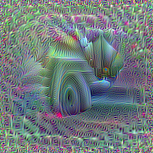
Zoom
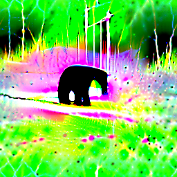
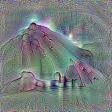
For zoom, we begin with an image of lower resolution than the desired result. In each step, we optimize this image for a fixed number of iterations and then up-sample the result, repeating until we reach the full resolution. Figure 2 shows the state of an image at each step of the zoom procedure, along with an image produced without zoom. The latter image splits the object of interest at its edges. By contrast, zoom appears to find a meaningful structure for the image in the early steps and refines details like texture as the resolution increases.
We note that zoom is not an entirely novel idea in inversion. Yin et al. (2020) use a similar technique as ‘warm-up’ for better performance and speed-up. However, we observe that continuing zoom throughout optimization contributes to the overall success of PII.
| Z | Z + C | C | None | Z | Z + C | C | None |
|---|---|---|---|---|---|---|---|

|

|

|

|

|

|

|

|
| w/ ColorShift | w/o ColorShift | ||||||
Zoom + Centering
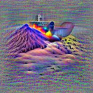
Unsurprisingly, we have found that applying zoom and centering simultaneously yields even better results than applying either individually, since each one provides a different benefit. Centering places detailed and important features (e.g. the dog’s eye in Figure 1) near the center and builds the rest of the image around the existing patch. Zoom helps enforce a sound large-scale structure for the image and fills in details later.
The combined Zoom and Centering process proceeds in ‘stages’, each at a higher resolution than the last. Each stage begins with an image patch generated by the previous stage, which approximately minimizes the inversion loss. The patch is then up-sampled to a resolution halfway between the previous stage and current stage resolution, filling the center of the image and leaving a border which is padded with random noise. The next round of optimization then begins starting from this newly processed image.
3.2 ColorShift Augmentation
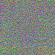
The colors of the illustrative images we have shown so far are notably different from what one might expect in a natural image. This is due to ColorShift, a new augmentation that we now present.
ColorShift is an adjustment of an image’s colors by a random mean and variance in each channel. This can be formulated as follows:
where and are -dimensional111 being the number of channels vectors drawn from and , respectively, and are repeatedly redrawn after a fixed number of iterations. We use in all demonstrations unless otherwise noted. At first glance, this deliberate shift away from the distribution of natural images seems counterproductive to the goal of producing a recognizable image. However, our results show that using ColorShift noticeably increases the amount of visual information in inverted images and also obviates the need for hard-to-tune regularizers to stabilize optimization.
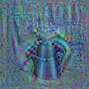
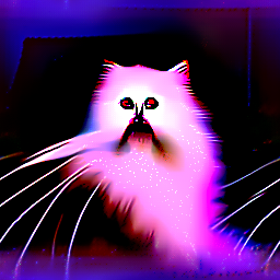
We visualize the stabilizing effect of ColorShift in Figure 3. In this experiment, we invert the model by minimizing the sum of a cross entropy and a total-variation (TV) penalty. Without ColorShift, the quality of images is highly dependent on the weight of the TV regularizer; smaller values produce noisy images, while larger values produce blurry ones. Inversion with ColorShift, on the other hand, is insensitive to this value and in fact succeeds when omitting the regularizer altogether.
Other preliminary experiments show that ColorShift similarly removes the need for or feature regularization, as our main results for PII will show. We conjecture that by forcing unnatural colors into an image, ColorShift requires the optimization to find a solution which contains meaningful semantic information, rather than photo-realistic colors, in order to achieve a high class score. Alternatively, as seen in Figure 10, images optimized with an image prior may achieve high scores despite a lack of semantic information merely by finding sufficiently natural colors and textures.
3.3 Ensembling
Ensembling is an established tool often used in applications from enhanced inference (Opitz & Maclin, 1999) to dataset security (Souri et al., 2021). We find that optimizing an ensemble composed of different ColorShifts of the same image simultaneously improves the performance of inversion methods. To this end, we minimize the average of cross-entropy losses , where the are different ColorShifts of the image at the current step of optimization. Figure 4 shows the result of applying ensembling alongside ColorShift. We observe that larger ensembles appear to give slight improvements, but even ensembles of size 1 or two produce satisfactory results. This is important for models like ViTs, where available GPU memory constrains the possible size of this ensemble; in general, we use the largest ensemble size (up to a maximum of ) that our hardware permits for a particular model. More results on the effect of ensemble size can be found in Figure 15. We show the effect of ensembling using other well-known augmentations and compare them to ColorShift in Appendix Section A.5, and observe that ColorShift is the strongest among augmentations we tried for model inversion.
3.4 The Plug-in Inversion Method
We combine the jitter, ensembling, ColorShift, centering, and zoom techniques, and name the result Plug-In Inversion, which references the ability to ‘plug in’ any differentiable model, including ViTs and MLPs, using a single fixed set of hyper-parameters. Full pseudocode for the algorithm may be found in appendix E. In the next section, we detail the experimental method that we used to find these hyper-parameters, after which we present our main results.
 |
 |
 |
 |
 |
| ResNet-101 | ViT B-32 | DeiT P16 224 | Deit Dist P16 384 | ConViT tiny |
 |
 |
 |
 |
 |
| Mixer b16 224 | PiT Dist 224 | ResMLP 36 Dist | Swin P4 W12 | Twin PCPVT |
| Barn | Garbage | Goblet | Ocean | CRT | Warplane | |
|---|---|---|---|---|---|---|
| Truck | Liner | Screen | ||||
| ResNet-101 |  |
 |
 |
 |
 |
 |
| ViT B-32 |  |
 |
 |
 |
 |
 |
| DeiT Dist |  |
 |
 |
 |
 |
 |
| ResMLP 36 |  |
 |
 |
 |
 |
 |
| Apple | Castle | Dolphin | Maple | Road | Rose | Sea | Seal | Train | |
|---|---|---|---|---|---|---|---|---|---|
| ViT L-16 |  |
 |
 |
 |
 |
 |
 |
|
 |
| ViT B-32 | |
|
|
|
|
|
|
|
|
| ViT S-32 | |
|
|
|
|
|
|
|
|
| ViT T-16 | |
|
|
|
|
|
|
|
|
| Plane | Car | Bird | Cat | Deer | Dog | Frog | Horse | Ship | Truck | |
|---|---|---|---|---|---|---|---|---|---|---|
| ViT L-32 | |
 |
 |
 |
 |
 |
 |
 |
 |
 |
| ViT L-16 | |
|
|
|
|
|
|
|
|
|
| ViT B-32 | |
|
|
|
|
|
|
|
|
|
| ViT B-16 | |
|
|
|
|
|
|
|
|
|
4 Experimental Setup
In order to tune hyper-parameters of PII for use on naturally-trained models, we use the torchvision (Paszke et al., 2019) ImageNet-trained ResNet-50 model. We apply centering + zoom simultaneously in 7 ‘stages’. During each stage, we optimize the selected patch for 400 iterations, applying random jitter and ColorShift at each step. We use the Adam (Kingma & Ba, 2014) optimizer with momentum , initial learning rate , and cosine-decay. At the beginning of every stage, the learning rate and optimizer are re-initialized. We use for the ColorShift parameters, and an ensemble size of . Further ablation studies for these choices can be found in figures 11, 14, and 15.
All the models (including pre-trained weights) we consider in this work are publicly available from widely-used sources. Explicit details of model resources can be found in section B of the appendix. We also make the code used for all demonstrations and experiments in this work available at https://github.com/youranonymousefriend/plugininversion.
5 Results
5.1 PII works on a range of architectures
We now present the results of applying Plug-In Inversion to different types of models. We once again emphasize that we use identical settings for the PII parameters in all cases.
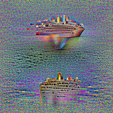
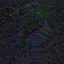
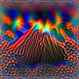
Figure 6 depicts images produced by inverting the Volcano class for a variety of architectures, including examples of CNNs, ViTs, and MLPs. While the quality of images varies somewhat between networks, all of them include distinguishable and well-placed visual information. Many more examples are found in Figure 17 of the Appendix.
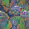
In Figure 7, we show images produced by PII from representatives of each main type of architecture for a few arbitrary ImageNet classes. We note the distinct visual styles that appear in each row, which supports the perspective of model inversion as a tool for understanding what kind of information different networks learn during training.
| Gown | Microphone | Mobile Home | Schooner | Cardoon | Volcano |
|---|---|---|---|---|---|
PII

|
|
|
|
|
|
PII + DeepInv

|
|
|
|
|
|
DeepInv

|
|
|
|
|
|
5.2 PII works on other datasets
In Figure 8, we use PII to invert ViT models trained on ImageNet and fine-tuned on CIFAR-100. Figure 9 shows inversion results from models fine-tuned on CIFAR-10. We emphasize that these were produced using identical settings to the ImageNet results above, whereas other methods (like DeepInversion) tune dataset-specific hyperparameters.
5.3 Comparing PII to existing methods
To quantitatively evaluate our method, we invert both a pre-trained ViT model and a pretrained ResMLP model to produce one image per class using PII, and do the same using DeepDream (i.e., DeepInversion minus feature regularization, which is not available for this model). We then use a variety of pre-trained models to classify these images. Table 1(b) contains the mean top-1 and top-5 classification accuracies across these models, as well as Inception scores, for the generated images from each method. We see that our method is competitive with, and in the ViT case widely outperforms, DeepDream. Appendix G contains more details about these experiments.
| Method | Inception score | Top-1 | Top-5 |
|---|---|---|---|
| PII | 28.17 7.21 | 77.0% | 89.5% |
| DeepDream | 2.72 0.23 | 35.2% | 49.6% |
| Method | Inception score | Top-1 | Top-5 |
|---|---|---|---|
| PII | 49.2% | 62.0% | |
| DeepDream | 51.3% | 61.3% |
Figure 10 shows images from a few arbitrary classes produced by PII and DeepInversion. We additionally show images produced by DeepInversion using the output of PII, rather than random noise, as its initialization. Using either initialization, DeepInversion clearly produces images with natural-looking colors and textures, which PII of course does not. However, DeepInversion alone results in some images that either do not clearly correspond to the target class or are semantically confusing. By comparison, PII again produces images with strong spatial and semantic qualities. Interestingly, these qualities appear to be largely retained when applying DeepInversion after PII, but with the color and texture improvements that image priors afford (Mahendran & Vedaldi, 2015), suggesting that using these methods in tandem may be a way to produce even better inverted images from CNNs than either method independently.
Appendix F contains additional qualitative comparisons to DeepDream and DeepInversion, further illustrating the need for model-specific hyperparameter tuning in contrast to our method.
6 Conclusion
We studied the effect of various augmentations on the quality of class-inverted images and introduced Plug-In Inversion, which uses these augmentations in tandem. We showed that this technique produces intelligible images from a wide range of well-studied architectures and datasets, including the recently introduced ViTs and MLPs, without a need for model-specific hyper-parameter tuning. We believe that augmentation-based model inversion is a promising direction for future research in understanding computer vision models.
References
- Chen et al. (2020) Chen, X., Fan, H., Girshick, R., and He, K. Improved baselines with momentum contrastive learning. arXiv preprint arXiv:2003.04297, 2020.
- Chu et al. (2021) Chu, X., Tian, Z., Wang, Y., Zhang, B., Ren, H., Wei, X., Xia, H., and Shen, C. Twins: Revisiting the design of spatial attention in vision transformers. arXiv preprint arXiv:2104.13840, 1(2):3, 2021.
- d’Ascoli et al. (2021) d’Ascoli, S., Touvron, H., Leavitt, M., Morcos, A., Biroli, G., and Sagun, L. Convit: Improving vision transformers with soft convolutional inductive biases. arXiv preprint arXiv:2103.10697, 2021.
- Deng et al. (2009) Deng, J., Dong, W., Socher, R., Li, L.-J., Li, K., and Fei-Fei, L. Imagenet: A large-scale hierarchical image database. In 2009 IEEE conference on computer vision and pattern recognition, pp. 248–255. Ieee, 2009.
- Dosovitskiy & Brox (2016) Dosovitskiy, A. and Brox, T. Inverting visual representations with convolutional networks. In Proceedings of the IEEE conference on computer vision and pattern recognition, pp. 4829–4837, 2016.
- Dosovitskiy et al. (2021) Dosovitskiy, A., Beyer, L., Kolesnikov, A., Weissenborn, D., Zhai, X., Unterthiner, T., Dehghani, M., Minderer, M., Heigold, G., Gelly, S., Uszkoreit, J., and Houlsby, N. An image is worth 16x16 words: Transformers for image recognition at scale, 2021.
- Fredrikson et al. (2015) Fredrikson, M., Jha, S., and Ristenpart, T. Model inversion attacks that exploit confidence information and basic countermeasures. In Proceedings of the 22nd ACM SIGSAC conference on computer and communications security, pp. 1322–1333, 2015.
- He et al. (2016) He, K., Zhang, X., Ren, S., and Sun, J. Deep residual learning for image recognition. In Proceedings of the IEEE conference on computer vision and pattern recognition, pp. 770–778, 2016.
- Heo et al. (2021) Heo, B., Yun, S., Han, D., Chun, S., Choe, J., and Oh, S. J. Rethinking spatial dimensions of vision transformers. arXiv preprint arXiv:2103.16302, 2021.
- Howard et al. (2019) Howard, A., Sandler, M., Chu, G., Chen, L.-C., Chen, B., Tan, M., Wang, W., Zhu, Y., Pang, R., Vasudevan, V., et al. Searching for mobilenetv3. In Proceedings of the IEEE/CVF International Conference on Computer Vision, pp. 1314–1324, 2019.
- Huang et al. (2017) Huang, G., Liu, Z., Van Der Maaten, L., and Weinberger, K. Q. Densely connected convolutional networks. In Proceedings of the IEEE conference on computer vision and pattern recognition, pp. 4700–4708, 2017.
- Iandola et al. (2016) Iandola, F. N., Han, S., Moskewicz, M. W., Ashraf, K., Dally, W. J., and Keutzer, K. Squeezenet: Alexnet-level accuracy with 50x fewer parameters and¡ 0.5 mb model size. arXiv preprint arXiv:1602.07360, 2016.
- Ioffe & Szegedy (2015) Ioffe, S. and Szegedy, C. Batch normalization: Accelerating deep network training by reducing internal covariate shift. In International conference on machine learning, pp. 448–456. PMLR, 2015.
- Kingma & Ba (2014) Kingma, D. P. and Ba, J. Adam: A method for stochastic optimization. arXiv preprint arXiv:1412.6980, 2014.
- Krizhevsky et al. (2012) Krizhevsky, A., Sutskever, I., and Hinton, G. E. Imagenet classification with deep convolutional neural networks. Advances in neural information processing systems, 25:1097–1105, 2012.
- LeCun et al. (1989) LeCun, Y., Boser, B., Denker, J. S., Henderson, D., Howard, R. E., Hubbard, W., and Jackel, L. D. Backpropagation applied to handwritten zip code recognition. Neural computation, 1(4):541–551, 1989.
- Liu et al. (2021a) Liu, H., Dai, Z., So, D. R., and Le, Q. V. Pay attention to mlps. arXiv preprint arXiv:2105.08050, 2021a.
- Liu et al. (2021b) Liu, Z., Lin, Y., Cao, Y., Hu, H., Wei, Y., Zhang, Z., Lin, S., and Guo, B. Swin transformer: Hierarchical vision transformer using shifted windows. arXiv preprint arXiv:2103.14030, 2021b.
- Ma et al. (2018) Ma, N., Zhang, X., Zheng, H.-T., and Sun, J. Shufflenet v2: Practical guidelines for efficient cnn architecture design. In Proceedings of the European conference on computer vision (ECCV), pp. 116–131, 2018.
- Mahendran & Vedaldi (2015) Mahendran, A. and Vedaldi, A. Understanding deep image representations by inverting them. In Proceedings of the IEEE conference on computer vision and pattern recognition, pp. 5188–5196, 2015.
- Mejia et al. (2019) Mejia, F. A., Gamble, P., Hampel-Arias, Z., Lomnitz, M., Lopatina, N., Tindall, L., and Barrios, M. A. Robust or private? adversarial training makes models more vulnerable to privacy attacks. arXiv preprint arXiv:1906.06449, 2019.
- Mordvintsev et al. (2015) Mordvintsev, A., Olah, C., and Tyka, M. Inceptionism: Going deeper into neural networks. 2015.
- Olah et al. (2017) Olah, C., Mordvintsev, A., and Schubert, L. Feature visualization. Distill, 2017. doi: 10.23915/distill.00007. https://distill.pub/2017/feature-visualization.
- Opitz & Maclin (1999) Opitz, D. and Maclin, R. Popular ensemble methods: An empirical study. Journal of artificial intelligence research, 11:169–198, 1999.
- Paszke et al. (2019) Paszke, A., Gross, S., Massa, F., Lerer, A., Bradbury, J., Chanan, G., Killeen, T., Lin, Z., Gimelshein, N., Antiga, L., et al. Pytorch: An imperative style, high-performance deep learning library. Advances in neural information processing systems, 32:8026–8037, 2019.
- Salimans et al. (2016) Salimans, T., Goodfellow, I., Zaremba, W., Cheung, V., Radford, A., and Chen, X. Improved techniques for training gans. Advances in neural information processing systems, 29:2234–2242, 2016.
- Sandler et al. (2018) Sandler, M., Howard, A., Zhu, M., Zhmoginov, A., and Chen, L.-C. Mobilenetv2: Inverted residuals and linear bottlenecks. In Proceedings of the IEEE conference on computer vision and pattern recognition, pp. 4510–4520, 2018.
- Santurkar et al. (2019) Santurkar, S., Ilyas, A., Tsipras, D., Engstrom, L., Tran, B., and Madry, A. Image synthesis with a single (robust) classifier. Advances in Neural Information Processing Systems, 32:1262–1273, 2019.
- Shafahi et al. (2019) Shafahi, A., Najibi, M., Ghiasi, A., Xu, Z., Dickerson, J., Studer, C., Davis, L. S., Taylor, G., and Goldstein, T. Adversarial training for free! arXiv preprint arXiv:1904.12843, 2019.
- Simonyan & Zisserman (2014) Simonyan, K. and Zisserman, A. Very deep convolutional networks for large-scale image recognition. arXiv preprint arXiv:1409.1556, 2014.
- Simonyan et al. (2014) Simonyan, K., Vedaldi, A., and Zisserman, A. Deep inside convolutional networks: Visualising image classification models and saliency maps, 2014.
- Souri et al. (2021) Souri, H., Goldblum, M., Fowl, L., Chellappa, R., and Goldstein, T. Sleeper agent: Scalable hidden trigger backdoors for neural networks trained from scratch. arXiv preprint arXiv:2106.08970, 2021.
- Szegedy et al. (2015) Szegedy, C., Liu, W., Jia, Y., Sermanet, P., Reed, S., Anguelov, D., Erhan, D., Vanhoucke, V., and Rabinovich, A. Going deeper with convolutions. In Proceedings of the IEEE conference on computer vision and pattern recognition, pp. 1–9, 2015.
- Tan et al. (2019) Tan, M., Chen, B., Pang, R., Vasudevan, V., Sandler, M., Howard, A., and Le, Q. V. Mnasnet: Platform-aware neural architecture search for mobile. In Proceedings of the IEEE/CVF Conference on Computer Vision and Pattern Recognition, pp. 2820–2828, 2019.
- Tolstikhin et al. (2021) Tolstikhin, I., Houlsby, N., Kolesnikov, A., Beyer, L., Zhai, X., Unterthiner, T., Yung, J., Keysers, D., Uszkoreit, J., Lucic, M., et al. Mlp-mixer: An all-mlp architecture for vision. arXiv preprint arXiv:2105.01601, 2021.
- Touvron et al. (2021a) Touvron, H., Bojanowski, P., Caron, M., Cord, M., El-Nouby, A., Grave, E., Izacard, G., Joulin, A., Synnaeve, G., Verbeek, J., and Jégou, H. Resmlp: Feedforward networks for image classification with data-efficient training, 2021a.
- Touvron et al. (2021b) Touvron, H., Cord, M., Douze, M., Massa, F., Sablayrolles, A., and Jegou, H. Training data-efficient image transformers & distillation through attention. In International Conference on Machine Learning, volume 139, pp. 10347–10357, July 2021b.
- Touvron et al. (2021c) Touvron, H., Cord, M., Douze, M., Massa, F., Sablayrolles, A., and Jégou, H. Training data-efficient image transformers & distillation through attention. In International Conference on Machine Learning, pp. 10347–10357. PMLR, 2021c.
- Vaswani et al. (2017) Vaswani, A., Shazeer, N., Parmar, N., Uszkoreit, J., Jones, L., Gomez, A. N., Kaiser, Ł., and Polosukhin, I. Attention is all you need. In Advances in neural information processing systems, pp. 5998–6008, 2017.
- Wightman (2019) Wightman, R. Pytorch image models. https://github.com/rwightman/pytorch-image-models, 2019.
- Xie et al. (2017) Xie, S., Girshick, R., Dollár, P., Tu, Z., and He, K. Aggregated residual transformations for deep neural networks. In Proceedings of the IEEE conference on computer vision and pattern recognition, pp. 1492–1500, 2017.
- Xu et al. (2021) Xu, W., Xu, Y., Chang, T., and Tu, Z. Co-scale conv-attentional image transformers. arXiv preprint arXiv:2104.06399, 2021.
- Yin et al. (2020) Yin, H., Molchanov, P., Alvarez, J. M., Li, Z., Mallya, A., Hoiem, D., Jha, N. K., and Kautz, J. Dreaming to distill: Data-free knowledge transfer via deepinversion. In Proceedings of the IEEE/CVF Conference on Computer Vision and Pattern Recognition, pp. 8715–8724, 2020.
- Zagoruyko & Komodakis (2016) Zagoruyko, S. and Komodakis, N. Wide residual networks. arXiv preprint arXiv:1605.07146, 2016.
- Zeiler & Fergus (2014) Zeiler, M. D. and Fergus, R. Visualizing and understanding convolutional networks. In European conference on computer vision, pp. 818–833. Springer, 2014.
Appendix A Additional Results
A.1 Ablation Study for and
Figure 11 shows the results of PII when varying the values of and , which determine the intervals from which the ColorShift constants are randomly drawn. Based on this and similar experiments, we permanently fix these parameters to for all other PII experiments, and find that these values indeed transfer well to other models.

|

|

|

|
|

|

|
|

|

|

|

|

|
|

|
|

|

|

|

|

|

|

|
|

|

|

|

|

|

|

|
|

|

|

|

|

|

|

|
|

|

|

|

|

|

|

|
|

|

|

|

|

|

|

|
A.2 Insensitivity to TV regularization
Figure 12 shows additional results on the effect of ColorShift on the sensitivity to the weight of TV regularization when inverting a robust model, complementing Figure 3. As in the earlier figure, we observe that certain values of may produce noisy or blurred images when not using ColorShift, whereas the ColorShift results are quite stable.
| w/ CS |

|

|

|

|

|

|
| w/o CS |
|
|
|
|
|
|
| w/ CS |

|

|

|

|

|

|
| w/o CS |
|
|
|
|
|
|
| w/ CS |

|

|

|

|

|

|
| w/o CS |
|
|
|
|
|
|
| w/ CS |

|

|

|

|

|

|
| w/o CS |
|
|
|
|
|
|
A.3 Effect of Centering
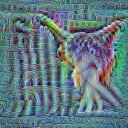
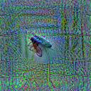
Figures 13 and 14 show the effect of centering on inverting a robust and natural model, respectively.
| Cen | Not Cen | Cen | Not Cen | Cen | Not Cen | Cen | Not Cen |

|

|

|
|

|

|

|

|
| Gold Finch | Box Turtle | Harvestman | Black Widow | ||||

|

|

|

|

|

|

|

|
| Black Grouse | Mergus Serrator | Border Terrier | Tiger Beetle | ||||

|

|

|

|

|

|

|

|
| Cricket | Upright Piano | Windsor Tie | Volcano | ||||
| Cen | Not Cen | Cen | Not Cen | Cen | Not Cen | Cen | Not Cen |

|

|

|
|
|

|

|

|
| Bustard | Otterhound | Fly | Macaque | ||||

|

|

|

|
|

|

|

|
| Clog | Combination Lock | Coffeepot | Espresso Maker | ||||

|

|

|

|

|

|

|

|
| Shower Curtain | TV | Iron | Mower | ||||
A.4 Effect of Ensemble Size
Figure 15 gives additional results to those in figure 4 for the effect of ensemble size on inversion.
| 403 |

|

|

|

|

|

|

|
| 283 |

|

|

|

|

|

|
|
| 449 |

|

|

|

|

|

|

|
| 460 |

|

|

|

|

|

|

|
| 558 |

|

|

|

|

|

|

|
| 802 |

|

|

|

|

|

|

|
| 834 |

|

|

|

|

|

|

|
A.5 Effect of using other Augmentations
We used 4 random augmentations other than ColorShift to make comparisons. We used augmentations used in (Chen et al., 2020) with modifications. We use PyTorch (Paszke et al., 2019) notation to describe this part. We used RandomHorizontalFlip with 0.5 probability. We used RandomResizedCrop with scale [0.7, 1.], and ratio [0.75, and 1.33]. With applied ColorJitter with 0.8 probability, and brightness, contrast, saturation, and hue of (0.4, 0.4, 0.4, 0.1), respectively. We used RandomGrayscale with 0.2 probability. For this experiment, we do apply data normalization before feeding the input to the network. This is different than the regular experiment setting that we use for the robust model (see appendix C). The reason is that not having data normalization is similar to using ColorShift (it changes the data distribution which the model expects as an input).
| No Aug | Flip | Crop | Gray | Color Jitter | ColorShift | |
| target=140 |

|

|

|

|

|

|
| target=295 |

|

|

|

|
|
|
| target=350 |

|

|

|

|

|

|
| target=240 |

|

|
|

|

|

|
| target=400 |

|

|

|

|

|

|
| target=460 |

|

|

|

|

|

|
A.6 PII on additional networks

|

|

|

|

|

|

|

|
| AlexNet | DenseNet | GoogLeNet | MobileNet v2 | MobileNet v3-l | MobileNet v3-s | MNasNet 0-5 | MNasNet 1-0 |

|

|

|

|

|
|

|

|
| ResNet 18 | ResNet 34 | ResNet 50 | ResNet 101 | ResNet 152 | ResNext 50 | ResNext 101 | WResNet 50 |

|

|

|

|

|

|

|

|
| WResNet 101 | ShuffleNet v2-0-5 | ShuffleNet v2-1-0 | SqueezeNet | VGG11-bn | VGG13-bn | VGG16-bn | VGG19-bn |

|

|

|

|

|

|
|

|
| ViT B16 | ViT B32 | ViT L16 | ViT L32 | DeiT p16-224 | DeiT-D p16-384 | Deit p16-384 | DeiT-D-t p16-224 |

|

|

|

|

|

|

|

|
| DeiT-D-s p16-224 | DeiT-D p16-224 | CoaT-m | CoaT-s | CoaT-t | ConViT | ConViT-s | ConViT-t |

|
|

|

|

|

|
|

|
| Mixer 24-224 | Mixer b16-224 | Mixer l16-224 | PiT-D b-224 | PiT s-224 | PiT-D s-224 | Pit-D t-224 | ResMLP 12-224 |

|

|

|

|

|

|

|

|
| ResMLP-D 12-224 | ResMLP 24-224 | ResMLP-D 24-224 | ResMLP 36-224 | ResMLP-D 36-224 | ResMLP b-24-224 | ResMLP b-24-224-1k | ResMLP-D b-24-224 |

|

|

|

|

|

|

|

|
| Swin w12-384 | Swin s-w7-224 | Twin pcpvt-b | Twin pcpvt-l | Twin pcpvt-s | Twin svt-b | Twin svt-l | Twin svt-s |
Appendix B Models
In our experiments, we use publicly available pre-trained models from various sources. The following tables list the models used from each source, along with references to where they are introduced in the literature.
| Alias | Name | Paper |
|---|---|---|
| ViT B16 | B_16_imagenet1k | (Dosovitskiy et al., 2021) |
| ViT B32 | B_32_imagenet1k | (Dosovitskiy et al., 2021) |
| ViT B-32 | B_32_imagenet1k | (Dosovitskiy et al., 2021) |
| ViT L16 | L_16_imagenet1k | (Dosovitskiy et al., 2021) |
| ViT L32 | L_32_imagenet1k | (Dosovitskiy et al., 2021) |
| Alias | Name | Paper |
|---|---|---|
| DeiT p16-224 | deit_base_patch16_224 | (Touvron et al., 2021c) |
| DeiT P16 224 | deit_base_patch16_224 | (Touvron et al., 2021c) |
| Deit-D p16-384 | deit_base_distilled_patch16_384 | (Touvron et al., 2021c) |
| Deit Dist P16 384 | deit_base_distilled_patch16_384 | (Touvron et al., 2021c) |
| deit p16-384 | deit_base_patch16_384 | (Touvron et al., 2021c) |
| Deit-D-t p16-224 | deit_tiny_distilled_patch16_224 | (Touvron et al., 2021c) |
| Deit-D-s p16-224 | deit_small_distilled_patch16_224 | (Touvron et al., 2021c) |
| Deit-D p16-224 | deit_base_distilled_patch16_224 | (Touvron et al., 2021c) |
| Alias | Name | Paper |
|---|---|---|
| AlexNet | alexnet | (Krizhevsky et al., 2012) |
| DenseNet | densenet121 | (Huang et al., 2017) |
| GoogLeNet | googlenet | (Szegedy et al., 2015) |
| MobileNet v2 | mobilenet_v2 | (Sandler et al., 2018) |
| MobileNet-v2 | mobilenet_v2 | (Sandler et al., 2018) |
| MobileNet v3-l | mobilenet_v3_large | (Howard et al., 2019) |
| MobileNet v3-s | mobilenet_v3_small | (Howard et al., 2019) |
| MNasNet 0-5 | mnasnet0_5 | (Tan et al., 2019) |
| MNasNet 1-0 | mnasnet1_0 | (Tan et al., 2019) |
| ResNet 18 | resnet18 | (He et al., 2016) |
| ResNet-18 | resnet18 | (He et al., 2016) |
| ResNet 34 | resnet34 | (He et al., 2016) |
| ResNet 50 | resnet50 | (He et al., 2016) |
| ResNet 101 | resnet101 | (He et al., 2016) |
| ResNet-101 | resnet101 | (He et al., 2016) |
| ResNet 152 | resnet152 | (He et al., 2016) |
| ResNext 50 | resnext50_32x4d | (Xie et al., 2017) |
| ResNext 101 | resnext101_32x8d | (Xie et al., 2017) |
| WResNet 50 | wide_resnet50_2 | (Zagoruyko & Komodakis, 2016) |
| WResNet 101 | wide_resnet101_2 | (Zagoruyko & Komodakis, 2016) |
| W-ResNet-101-2 | wide_resnet101_2 | (Zagoruyko & Komodakis, 2016) |
| ShuffleNet v2-0-5 | shufflenet_v2_x0_5 | (Ma et al., 2018) |
| ShuffleNet v2-1-0 | shufflenet_v2_x1_0 | (Ma et al., 2018) |
| ShuffleNet v2 | shufflenet_v2_x1_0 | (Ma et al., 2018) |
| SqueezeNet | squeezenet1_0 | (Iandola et al., 2016) |
| VGG11-bn | vgg11_bn | (Simonyan & Zisserman, 2014) |
| VGG13-bn | vgg13_bn | (Simonyan & Zisserman, 2014) |
| VGG16-bn | vgg16_bn | (Simonyan & Zisserman, 2014) |
| VGG19-bn | vgg19_bn | (Simonyan & Zisserman, 2014) |
| Alias | Name | Paper |
|---|---|---|
| CoaT-m | coat_lite_mini | (Xu et al., 2021) |
| CoaT-s | coat_lite_small | (Xu et al., 2021) |
| CoaT-t | coat_lite_tiny | (Xu et al., 2021) |
| ConViT | convit_base | (d’Ascoli et al., 2021) |
| ConViT-s | convit_small | (d’Ascoli et al., 2021) |
| ConViT-t | convit_tiny | (d’Ascoli et al., 2021) |
| ConViT tiny | convit_tiny | (d’Ascoli et al., 2021) |
| Mixer 24-224 | mixer_24_224 | (Tolstikhin et al., 2021) |
| Mixer b16-224 | mixer_b16_224 | (Tolstikhin et al., 2021) |
| Mixer b16 224 | mixer_b16_224 | (Tolstikhin et al., 2021) |
| Mixer b16-224-mill | mixer_b16_224_miil | (Tolstikhin et al., 2021) |
| Mixer l16-224 | mixer_l16_224 | (Tolstikhin et al., 2021) |
| PiT-D b-224 | pit_b_distilled_224 | (Heo et al., 2021) |
| PiT Dist 224 | pit_b_distilled_224 | (Heo et al., 2021) |
| PiT s-224 | pit_s_224 | (Heo et al., 2021) |
| PiT-D s-224 | pit_s_distilled_224 | (Heo et al., 2021) |
| PiT-D t-224 | pit_ti_distilled_224 | (Heo et al., 2021) |
| ResMLP 12-224 | resmlp_12_224 | (Touvron et al., 2021a) |
| ResMLP-D 12-224 | resmlp_12_distilled_224 | (Touvron et al., 2021a) |
| ResMLP 24-224 | resmlp_24_224 | (Touvron et al., 2021a) |
| ResMLP-D 24-224 | resmlp_24_distilled_224 | (Touvron et al., 2021a) |
| ResMLP 36-224 | resmlp_36_224 | (Touvron et al., 2021a) |
| ResMLP-D 36-224 | resmlp_36_distilled_224 | (Touvron et al., 2021a) |
| ResMLP 36 Dist | resmlp_36_distilled_224 | (Touvron et al., 2021a) |
| ResMLP b-24-224 | resmlp_big_24_224 | (Touvron et al., 2021a) |
| ResMLP b-24-224-1k | resmlp_big_24_224_in22ft1k | (Touvron et al., 2021a) |
| ResMLP-D b-24-224 | resmlp_big_24_distilled_224 | (Touvron et al., 2021a) |
| Swin w7-224 | swin_base_patch4_window7_224 | (Liu et al., 2021b) |
| Swin l-w7-224 | swin_large_patch4_window7_224 | (Liu et al., 2021b) |
| Swin l-w12-384 | swin_large_patch4_window12_384 | (Liu et al., 2021b) |
| Swin w12-384 | swin_base_patch4_window12_384 | (Liu et al., 2021b) |
| Swin P4 W12 | swin_base_patch4_window12_384 | (Liu et al., 2021b) |
| Swin s-w7-224 | swin_small_patch4_window7_224 | (Liu et al., 2021b) |
| Swin t-w7-224 | swin_tiny_patch4_window7_224 | (Liu et al., 2021b) |
| Twin pcpvt-b | twins_pcpvt_base | (Chu et al., 2021) |
| Twin PCPVT | twins_pcpvt_base | (Chu et al., 2021) |
| Twins pcpvt-l | twins_pcpvt_large | (Chu et al., 2021) |
| Twins pcpvt-s | twins_pcpvt_small | (Chu et al., 2021) |
| Twins svt-b | twins_svt_base | (Chu et al., 2021) |
| Twins svt-l | twins_svt_large | (Chu et al., 2021) |
| Twins svt-s | twins_svt_small | (Chu et al., 2021) |
Appendix C Additional experimental setting
C.1 Robust models
We use a robust RestNet-50 (He et al., 2016) model free-trained (Shafahi et al., 2019) on the ImageNet dataset (Deng et al., 2009). The setting we use for inverting robust models is very similar to that of PII explained in section 4 except for some differences. Throughout the paper, we use centering for robust models unless otherwise is mentioned (like when we are examining the effect of zoom and centering themselves). We use 0.0005 to scale total variation in the loss function. Also, we do not apply the data normalization layer before feeding the input to the network. In PII experiment setting, we apply a random ColorShift at each optimization step to each element in the ensemble. In the robust setting, we do not update the ColorShift variables , and for a fixed patch size, and we update these variables for the ensemble when we use a new patch size. Although using ColorShift would alleviate the need for using TV regularization as discussed in section 3.2, and illustrated in figure 3, we retain the TV penalty in our robust setting to make this setting more similar to that of previous inversion methods and to emphasize that it is a toy example for our ablation studies.
Appendix D Every Class of ImageNet Dataset Inverted


Appendix E Optimization algorithm
Input :
Model , class , final resolution , ColorShift parameters , ‘ensemble’ size , randomly initialized
for do
Pad with random noise to resolution
for do
for do
Appendix F Additional baseline comparisons
| MobileNet-v2 | ResNet-18 | VGG16-bn | W- ResNet-101-2 | ShuffleNet-v2 |
|
|
|
|
|
| ResNet-101 | ViT B-32 | DeiT P16 224 | Deit Dist P16 384 | ConViT tiny |
|
|
|
|
|
| Mixer b16 224 | PiT Dist 224 | ResMLP 36 Dist | Swin P4 W12 | Twin PCPVT |
| Barn | Garbage | Goblet | Ocean | CRT | Warplane | |
|---|---|---|---|---|---|---|
| Truck | Liner | Screen | ||||
| ResNet-101 |  |
 |
 |
 |
 |
 |
| ViT B-32 |  |
 |
 |
 |
 |
 |
| DeiT Dist |  |
 |
 |
 |
 |
 |
| ResMLP 36 | 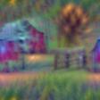 |
 |
 |
 |
 |
 |
Appendix G Quantitative Results
To quantitatively evaluate our method, we invert a pre-trained ViT model to produce one image per class using PII, and do the same using DeepDream (i.e., DeepInversion minus feature regularization, which is not available for this model). We then use a variety of pre-trained CNN, ViT, and MLP models to classify these images. We find that every model achieves strictly higher top-1 and top-5 accuracy on the PII-generated image set (excepting the ‘teacher’ model, which perfectly classifies both). We compile these results in figure 26. Additionally, we compute the Inception score (Salimans et al., 2016) for both sets of images, which also favors PII over DeepDream, with scores of and , respectively.


We also perform the same evaluation for images generated from a pre-trained ResMLP model. These results are more mixed; DeepDream images are classified much better by a small number of models, but the majority of models classify PII images better, and the average accuracy across models is approximately equal for both methods. Inception score, however, once again clearly favors PII over DeepDream, with scores of and , respectively.

