PKF: Probabilistic Data Association Kalman Filter for Multi-Object Tracking

Hanwen Cao¹ George J. Pappas² Nikolay Atanasov¹
¹University of California San Diego ²University of Pennsylvania

Abstract

In this paper, we derive a new Kalman filter with probabilistic data association between measurements and states. We formulate a variational inference problem to approximate the posterior density of the state conditioned on the measurement data. We view the unknown data association as a latent variable and apply Expectation Maximization (EM) to obtain a filter with update step in the same form as the Kalman filter but with expanded measurement vector of all potential associations. We show that the association probabilities can be computed as permanents of matrices with measurement likelihood entries. We also propose an ambiguity check that associates only a subset of ambiguous measurements and states probabilistically, thus reducing the association time and preventing low-probability measurements from harming the estimation accuracy. Experiments in simulation show that our filter achieves lower tracking errors than the well-established joint probabilistic data association filter (JPDAF), while running at comparable rate. We also demonstrate the effectiveness of our filter in multi-object tracking (MOT) on multiple real-world datasets, including MOT17, MOT20, and DanceTrack. We achieve better higher order tracking accuracy (HOTA) than previous Kalman-filter methods and remain real-time. Associating only bounding boxes without deep features or velocities, our method ranks top-10 on both MOT17 and MOT20 in terms of HOTA. Given offline detections, our algorithm tracks at 250+ fps on a single laptop CPU. Code is available at https://github.com/hwcao17/pkf.

1 Introduction

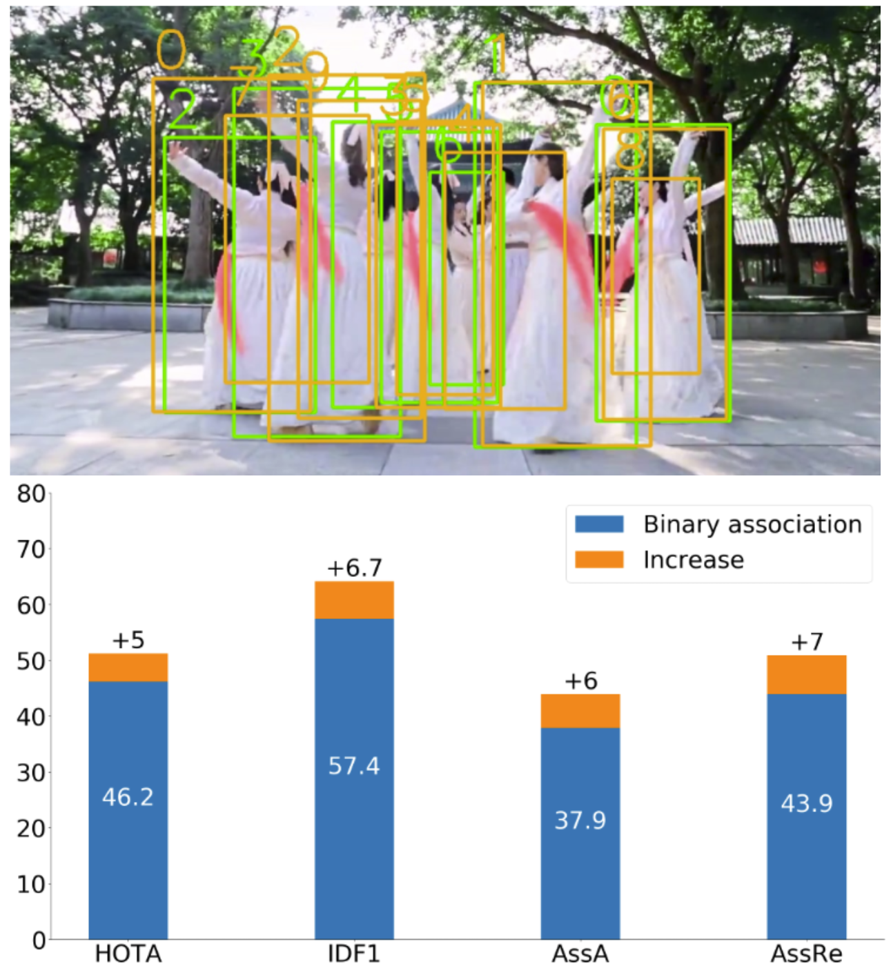
Refer to caption — Figure 1: Example scene with high ambiguity in DanceTrack [40] with green box detections and orange box tracks. Applying our probabilistic data association Kalman filter on this sequence significantly increases the association quality according to IDF1 [38], association accuracy (AssA) [24], association recall (AssRe) [24], and the combined HOTA metric [24].

In tasks where ambiguity exists between measurements and variables of interest, probabilistic data association can prevent catastrophic estimation failures. For example, in multi-object tracking (MOT), there can be a lot of occlusions causing high ambiguity in data association. An illustration of how probabilistic data association improves MOT is shown in Figure 1. Methods utilizing the Kalman filter [6, 47, 13] have achieved outstanding performance in MOT but have not considered the impact of probabilistic data association on the tracking process.

We derive a new formulation of the Kalman filter with probabilistic data association. Previous works [3, 12] show that the Kalman filter can be derived using variational inference (VI) by maximizing the evidence lower bound (ELBO) of the input and measurement data likelihood. To deal with ambiguous associations, we approach the VI problem using Expectation-Maximization (EM) with the data association as the latent variable. In the E-step, we show that the association weights can be computed as permanents of matrices with measurement likelihood entries using accelerated permanent algorithms [32, 20]. We also show that the weight computation can be extended to cases with missing detections and clutter. In the M-step, optimizing the EM objective once leads to a Kalman filter with the usual prediction and update steps but with an extended measurement vector and noise covariance matrix capturing all possible data associations. Our formulation is related to the well-known joint probabilistic data association filter (JPDAF) [2]. However, while JPDAF first computes a posterior given each associated measurement, i.e., maximizes the ELBO of each measurement, and then computes the weighted average of the posteriors, our filter directly optimizes the overall ELBO weighted by the data association probabilities. We show that our algorithm achieves lower tracking errors than JPDAF, while running at comparable tracking rates.

We also apply our filter to MOT. We observe that, with accurate detection algorithms [36, 35], binary associations are fast and work well when the ambiguity is not severe and incorporating measurements with low association weights can harm the estimation accuracy. Therefore, we employ a hybrid data association procedure. We first do binary data association (e.g., via [23, 21]) and then perform an ambiguity check which outputs a set of ambiguous measurements and tracks. Then, probabilistic data association is only performed on the ambiguous set, thus reducing the computation time and preventing low-probability measurements from harming the accuracy. We test our algorithm on multiple real-world MOT datasets, including MOT17 [27], MOT20 [15], and DanceTrack [40]. Our method outperforms previous Kalman-filter methods [47, 13] while maintaining almost the same inference speed. We name our probabilistic data association Kalman filter the PKF with P emphasizing both the probabilistic nature of the data association and the matrix permanent computation of the association weights. Our contributions are summarized as follows.

•

We formulate state estimation with ambiguous measurements as a VI problem and use EM to derive the PKF, a new Kalman filter with probabilistic data association.
•

We show that association probabilities can be computed using matrix permanents and design a hybrid association procedure with an ambiguity check to reduce computation complexity and exclude low-probability associations.
•

We demonstrate the effectiveness of the PKF in comparison to the JPDAF and on multiple real-world MOT datasets. PKF ranks top-10 on both MOT17 and MOT20 by associating only bounding boxes and runs at 250+ fps on a single laptop CPU given offline detections.

2 Related work

Probabilistic data association

Data association is a key challenge in estimation problems where measurements need to be related to estimated variables. The most straightforward association approach is by a nearest neighbor rule based on some distance metric, such as Euclidean or Mahalonobis [22]. However, nearest-neighbor associations are prone to mistakes. The joint compatibility branch and bound (JCBB) algorithm [31] computes a joint Mahalonobis distance and performs a joint $\chi^{2}$ test for the association event to obtain robust associations. To deal with ambiguity, Bar-Shalom and Tse developed the probabilistic data association filter (PDAF) [1] for tracking single objects in the presence of clutter measurements. In the Kalman filter update step, the innovation terms are computed for each of the possible associations and are averaged weighted by the association probabilities. The performance of PDAF can degrade in the multi-object case because its separate association process can cause multiple tracks to latch onto the same object. The JPDAF [2] extends the PDAF by associating all measurements and tracks jointly. In each association event, a measurement can be associated with at most one track, and vice versa. Musicki et al. [30] develop an integrated probabilistic data association (IPDA) method using a Markov chain modeling probabilistic data association, track initialization, and termination. JIPDA [29] extends IPDA [30] to the multi-object case by performing data association jointly. There are also improvements on the original JPDAF [2] like avoiding coalescence [8] and speeding up the inference [44, 37]. Meyer et al. [26] approach probabilistic data association using a factor graph where the variables (including objects and association events) and functions (motion, observation, et al.) are nodes and the edges model their relationships. The association probabilities can be computed efficiently by message passing in the graph. A survey of data association techniques can be found in [34]. Besides MOT, probabilistic data association is also applied in other estimation tasks like biological data processing [18] and simultaneous localization and mapping [9, 16].

Multi-object tracking State-of-art MOT algorithms are dominated by the tracking-by-detection approach, which consists of two steps: object detection [36, 35] and data association. SORT [6] uses the Hungarian algorithm [23] to associate bounding-box object detections and updates the object tracks using the Kalman filter to achieve real-time online tracking. DeepSORT [42] extends SORT [6] by introducing deep visual features for data association. ByteTrack [47] makes an observation that the detectors can make imperfect predictions in complex scenes and proposes a second round of data association for low-confidence detections. OC-SORT [13] analyzes the limitations of SORT [13], namely sensitivity to state noise and temporal error magnification, and proposes an observation-centric re-update step and object momentum for data association.

A second class of algorithms for MOT performs tracking-by-regression. Feichtenhofer et al. [17] use a correlation function between the feature maps of two frames to predict the transformation of bounding boxes in different frames. Bergmann et al. [4] uses the regression head of Faster-RCNN [36] to predict bounding-box offsets from the previous image to the current image. CenterTrack [49] adopts the same network architecture as CenterNet [48] but takes two consecutive images to predict object offsets between frames. Braso and Leal-Taixe [10] approach MOT with a graph neural network, which stores object features in the nodes and predicts whether two bounding boxes in different frames are the same object by edge features.

A third set of methods performs tracking-by-attention [25] using transformer models [41] for joint detection and tracking based on new object queries and tracked object queries, which solves the creation and association of objects implicitly. Although these methods utilize different techniques for data association, either explicit or implicit, they all consider deterministic data association.

3 Problem formulation

Consider $N$ time-varying variables that need to be estimated, denoted as $\mathbf{x}_{t,j}\in\mathbb{R}^{n}$ , $j=1,...,N$ . We refer to their concatenation into a single vector at time $t$ :

\mathbf{x}_{t}=\begin{bmatrix}\mathbf{x}_{t,1}^{\top}&\cdots&\mathbf{x}_{t,N}^{\top}\end{bmatrix}^{\top}\in\mathbb{R}^{nN}

(1)

as the state of a dynamical system. Suppose that $\mathbf{x}_{t}$ evolves according to a discrete-time linear motion model:

\mathbf{x}_{t+1}=F\mathbf{x}_{t}+G\mathbf{u}_{t}+\mathbf{w}_{t},\qquad\mathbf{w}_{t}\sim\mathcal{N}(\mathbf{0},W),

(2)

where $\mathbf{u}_{t}$ is the known input and $\mathbf{w}_{t}$ is zero-mean Gaussian noise with covariance $W$ .

At each time $t$ , a subset of the variables $\mathbf{x}_{t,1},\ldots,\mathbf{x}_{t,N}$ are observed. Let $M_{t}\in\{0,1,\ldots,N\}$ be the number of measurements at time $t$ and let $\mathbf{z}_{t,k}\in\mathbb{R}^{m}$ be the $k$ -th measurement with $k=1,\ldots,M_{t}$ , which is generated by some $\mathbf{x}_{t,j}$ according to a linear measurement model:

\mathbf{z}_{t,k}=H\mathbf{x}_{t,j}+\mathbf{v}_{t},\qquad\mathbf{v}_{t}\sim\mathcal{N}(\mathbf{0},V),

(3)

where $\mathbf{v}_{t}$ is zero-mean Gaussian noise with covariance $V$ . We denote the concatenation of all measurements by:

\mathbf{z}_{t}=\begin{bmatrix}\mathbf{z}_{t,1}^{\top}&\cdots&\mathbf{z}_{t,M_{t}}^{\top}\end{bmatrix}^{\top}\in\mathbb{R}^{mM_{t}}.

(4)

Problem.

Given an estimate of the state $\mathbf{x}_{t}$ at time $t$ , an input $\mathbf{u}_{t}$ , and measurements $\mathbf{z}_{t+1}$ , obtain an estimate of $\mathbf{x}_{t+1}$ . The association between the measurements $\mathbf{z}_{t+1,k}$ and the variables $\mathbf{x}_{t+1,j}$ that generated them is unknown.

4 Methodology

We formulate a Kalman filter with probabilistic data association to solve the estimation problem defined in Sec. 3.

4.1 Data association

We define the association between a set of measurements $\mathcal{Z}$ and a set of variables $\mathcal{X}$ that generated them as follows.

Definition.

The data association of set $\mathcal{Z}=\{\mathbf{z}_{k}\}_{k=1}^{M}$ to set $\mathcal{X}=\{\mathbf{x}_{j}\}_{j=1}^{N}$ is a function $\delta:\{1,\ldots,M\}\to\{0,1,\ldots,N\}$ that either associates an element $\mathbf{z}_{k}\in\mathcal{Z}$ to an element $\mathbf{x}_{\delta(k)}\in\mathcal{X}$ or indicates via $\delta(k)=0$ that there is no matching element in $\mathcal{X}$ .

For example, in MOT, $\mathcal{Z}$ is the set of measurements (e.g., features, bounding boxes, or object segmentations), and $\mathcal{X}$ is the set of tracked objects.

Let $\delta_{t}$ be the data association at time $t$ , such that measurement $\mathbf{z}_{t,k}$ is assigned to variable $\mathbf{x}_{t,\delta_{t}(k)}$ . We denote the set of all possible data association functions at time $t$ as $\mathcal{D}_{t}=\{\delta_{t}:\{1,...,M_{t}\}\to\{1,...,N\}\}$ and the set of data associations across all times as $\mathcal{D}=\cup_{t=1}^{T}\mathcal{D}_{t}$ .

We consider a probabilistic setting, in which we are given a prior probability density $p(\mathbf{x}_{t})$ of the state $\mathbf{x}_{t}$ , and aim to compute the posterior density $p(\mathbf{x}_{t+1}|\mathbf{z}_{t+1},\mathbf{u}_{t})$ of $\mathbf{x}_{t+1}$ conditioned on the input $\mathbf{u}_{t}$ and the measurements $\mathbf{z}_{t+1}$ . At each time $t$ , we treat the data association $\delta_{t}$ as a random variable with a uniform prior $p(\delta_{t})$ independent of $\mathbf{x}_{t}$ . Using Bayes rule and assuming the measurements are mutually independent conditioned on the variables that generated them, the density of $\delta_{t}$ conditioned on $\mathbf{z}_{t}$ satisfies:

$\displaystyle p(\delta_{t}\|\mathbf{z}_{t})$	$\displaystyle=\frac{p(\mathbf{z}_{t}\|\delta_{t})p(\delta_{t})}{p(\mathbf{z}_{t})}\propto p(\mathbf{z}_{t}\|\delta_{t})$
	$\displaystyle=\int p(\mathbf{z}_{t}\|\delta_{t},\mathbf{x}_{t})p(\mathbf{x}_{t})d\mathbf{x}_{t}$
	$\displaystyle=\prod_{k=1}^{M_{t}}\int p(\mathbf{z}_{t,k}\|\mathbf{x}_{t,\delta_{t}(k)})p(\mathbf{x}_{t,\delta_{t}(k)})d\mathbf{x}_{t,\delta_{t}(k)}$
	$\displaystyle=\prod_{k=1}^{M_{t}}p\left(\mathbf{z}_{t,k}\|\delta_{t}(k)\right).$	(5)

Let $p_{\mathcal{N}}(\cdot;\boldsymbol{\mu},\Sigma)$ denote the density of a Gaussian distribution with mean $\boldsymbol{\mu}$ and covariance $\Sigma$ . Since $p(\mathbf{z}_{t,k}|\mathbf{x}_{t,\delta_{t}(k)})=p_{\mathcal{N}}(\mathbf{z}_{t,k};H\mathbf{x}_{t,\delta_{t}(k)},V)$ and $p(\mathbf{x}_{t,\delta_{t}(k)})\allowbreak=p_{\mathcal{N}}(\mathbf{x}_{t,\delta_{t}(k)};\boldsymbol{\mu}_{t,\delta_{t}(k)},\Sigma_{t,\delta_{t}(k)})$ , we have:

p(\mathbf{z}_{t,k}|\delta_{t}(k))=p_{\mathcal{N}}(\mathbf{z}_{t,k};\!H\boldsymbol{\mu}_{t,\delta_{t}(k)},H\Sigma_{t,\delta_{t}(k)}H^{\top}+V).

Next, consider the likelihood that $\mathbf{z}_{t,k}$ is generated by $\mathbf{x}_{t,j}$ , which we denote by $w^{t}_{k,j}$ . Using (5), we have:

\displaystyle w^{t}_{k,j}=\!\!\!\!\sum_{\delta\in\mathcal{D}_{t}(k,j)}\!\!p(\delta|\mathbf{z}_{t})=\!\!\!\!\sum_{\delta\in\mathcal{D}_{t}(k,j)}\prod_{k^{\prime}=1}^{M_{t}}p\left(\mathbf{z}_{t,k^{\prime}}|\delta_{t}(k^{\prime})\right),

(6)

where $\mathcal{D}_{t}(k,j)$ is the set of data association functions that assign measurement $\mathbf{z}_{t,k}$ to variable $\mathbf{x}_{t,j}$ . We show that $w^{t}_{k,j}$ can be computed using the permanent of a matrix $Q$ containing the measurement likelihood $p(\mathbf{z}_{t,k}|\mathbf{x}_{t,j})$ as its entries $Q(k,j)$ . The permanent of a matrix $Q=\left[Q(k,j)\right]\in\mathbb{R}^{M\times N}$ with $M\leq N$ is defined as:

\operatorname*{per}(Q):=\sum_{\delta\in\mathcal{D}}\prod_{k=1}^{M}Q(k,\delta(k)),

(7)

where $\mathcal{D}$ is the set of injective functions $\delta:\{1,\ldots,M\}\to\{1,\ldots,N\}$ .

Proposition 1.

Let $Q^{t}\in\mathbb{R}^{M_{t}\times N}$ be a matrix with elements $Q^{t}(k,j)=p(\mathbf{z}_{t,k}|\delta_{t}(k)=j)=p(\mathbf{z}_{t,k}|\mathbf{x}_{t,j})$ . The data association weight $w^{t}_{k,j}$ in (6) can be computed as:

w^{t}_{k,j}\propto Q^{t}(k,j)\operatorname*{per}\left(Q^{t}_{-kj}\right),

(8)

where $Q^{t}_{-kj}$ is the matrix $Q^{t}$ with the $k$ -th row and $j$ -th column removed.

Proof.

See Supplementary Material Section 7. ∎

Proposition 1 allows us to compute data association weights. Next, we derive a Kalman filter with probabilistic data association.

4.2 Probabilistic data association Kalman filter

To derive a filter, we consider two time steps, namely $t$ and $t+1$ , and define a lifted form of the state:

\bar{\mathbf{x}}=\begin{bmatrix}\mathbf{x}_{t}^{\top}&\mathbf{x}_{t+1}^{\top}\end{bmatrix}^{\top}.

(9)

Given the prior density $p(\mathbf{x}_{t})$ , the input $\mathbf{u}_{t}$ , and the measurement $\mathbf{z}_{t+1}$ , we aim to find an estimate $q(\bar{\mathbf{x}})$ of the joint posterior $p(\bar{\mathbf{x}}|\mathbf{z}_{t+1},\mathbf{u}_{t})$ . To determine $q(\bar{\mathbf{x}})$ , we use variational inference [7, Ch. 10], which maximizes the ELBO of the evidence $\log p(\mathbf{z}_{t+1},\mathbf{u}_{t})$ with respect to $q(\bar{\mathbf{x}})$ . To save space, we denote $q(\bar{\mathbf{x}})$ by $q$ . The evidence can be decomposed as [7, Ch. 10]:

	$\displaystyle\log p(\mathbf{z}_{t+1},\mathbf{u}_{t})$	$\displaystyle=\operatorname*{KL}(q\|\|p(\bar{\mathbf{x}}\|\mathbf{z}_{t+1},\mathbf{u}_{t}))+\mathcal{L}(q),$		(10)
	$\displaystyle\mathcal{L}(q)$	$\displaystyle=\mathbb{E}_{q}\bigl{[}\log\frac{p(\bar{\mathbf{x}},\mathbf{z}_{t+1},\mathbf{u}_{t})}{q(\bar{\mathbf{x}})}\bigr{]},$		(11)

where $\operatorname*{KL}(q||p)$ is the Kullback–Leibler divergence and $\mathcal{L}(q)$ is the ELBO. Since the evidence is constant for given $\mathbf{z}_{t+1},\mathbf{u}_{t}$ , the ELBO is maximized when the $\operatorname*{KL}$ term is zero.

To account for probabilistic data association, we formulate the optimization inspired by the EM algorithm [7, Ch. 9]. EM determines the maximum likelihood (ML) or maximum a posterior (MAP) in the presence of unobserved variables. It contains an E-step that computes the expectation w.r.t. the unobserved variables and an M-step that maximizes the log-likelihood. Letting the data association $\delta_{t+1}$ be the unobserved variable, we consider the following optimization problem:

	$\displaystyle q^{(i+1)}\in\arg\max_{q}f^{(i)}(q),$		(12)
	$\displaystyle f^{(i)}(q)=\mathbb{E}_{\delta_{t+1}}\mathbb{E}_{\bar{\mathbf{x}}^{(i)}}\!\left[\mathcal{L}(q,\delta_{t+1})\mid\bar{\mathbf{x}}^{(i)},\mathbf{z}_{t+1}\right],$
	$\displaystyle\quad=\mathbb{E}_{\delta_{t+1}}\mathbb{E}_{\bar{\mathbf{x}}^{(i)}}\!\left[\mathbb{E}_{q}\bigl{[}\log\!\frac{p(\bar{\mathbf{x}},\mathbf{z}_{t+1},\mathbf{u}_{t},\delta_{t+1})}{q(\bar{\mathbf{x}})}\bigr{]}\mid\bar{\mathbf{x}}^{(i)}\!,\mathbf{z}_{t+1}\right],$

where the expectation $\mathbb{E}_{\bar{\mathbf{x}}^{(i)}}$ is with respect to $\bar{\mathbf{x}}^{(i)}\sim q^{(i)}(\bar{\mathbf{x}})$ . EM splits the optimization in (12) in two steps. The E-step requires computing the data association likelihood $p(\delta_{t+1}|\mathbf{z}_{t+1})$ . This can be obtained from (5) and Proposition 1. Given the data association weights $w^{t}_{k,j}$ , the M-step performs the optimization in (12) to determine $q^{(i+1)}$ .

We show that performing the E and M steps for one iteration, with initialization $\bar{\mathbf{x}}^{(i)}$ given by the prior state and the predicted state in (2), is equivalent to a Kalman filter with probabilistic data association. We first define an expanded observation model that captures all possible ways of generating the measurements at each time $t$ :

\bar{\mathbf{z}}_{t}=\bar{H}_{t}\mathbf{x}_{t}+\bar{\mathbf{v}}_{t},\qquad\bar{\mathbf{v}}_{t}\sim\mathcal{N}(\mathbf{0},\bar{V}_{t}),

(13)

where $\bar{\mathbf{z}}_{t}=(I_{M_{t}}\otimes\mathbf{1}_{N}\otimes I_{m})\mathbf{z}_{t}\in\mathbb{R}^{mM_{t}N}$ , $\bar{H}_{t}=\mathbf{1}_{M_{t}}\otimes\mathbf{I}_{N}\otimes H\in\mathbb{R}^{mM_{t}N\times nN}$ , $\mathbf{1}_{N}\in\mathbb{R}^{N}$ is a vector with elements equal to one, $\mathbf{I}_{N}\in\mathbb{R}^{N\times N}$ is the identity matrix, $\otimes$ is the Kronecker product, and $\bar{\mathbf{v}}_{t}$ is zero-mean Gaussian noise with covariance:

{\bar{V}_{t}\!=\!\!\begin{bmatrix}\bar{V}_{t,1}&\ &\ \\ \ &\ddots&\ \\ \ &\ &\bar{V}_{t,M_{t}}\end{bmatrix}\!\!,\bar{V}_{t,k}\!=\!\!\begin{bmatrix}V\!/\!w^{t}_{k,1}&\ &\ \\ \ &\ddots&\ \\ \ &\ &V\!/\!w^{t}_{k,N}\end{bmatrix}\!\!,}

(14)

where $w^{t}_{k,j}$ are the data association weights in (6). Using the expanded measurement model in (13), we obtain a Kalman filter with probabilistic data association.

Proposition 2.

Given prior $\mathbf{x}_{t}\sim\mathcal{N}(\boldsymbol{\mu}_{t},\Sigma_{t})$ and input $\mathbf{u}_{t}$ , the predicted Gaussian distribution $\mathcal{N}(\boldsymbol{\mu}_{t+1}^{+},\Sigma_{t+1}^{+})$ of $\mathbf{x}_{t+1}$ computed by the Kalman filter with motion model in (2) has parameters:

	$\displaystyle\boldsymbol{\mu}_{t+1}^{+}$	$\displaystyle=F\boldsymbol{\mu}_{t}+G\mathbf{u}_{t},$		(15)
	$\displaystyle\Sigma_{t+1}^{+}$	$\displaystyle=F\Sigma_{t}F^{\top}+W.$		(15)

Given measurements $\mathbf{z}_{t+1}$ , the updated Gaussian distribution $\mathcal{N}(\boldsymbol{\mu}_{t+1},\Sigma_{t+1})$ of $\mathbf{x}_{t+1}$ conditioned on $\mathbf{z}_{t+1}$ computed by the Kalman filter with probabilistic data association is obtained from the expanded measurement model in (13) as:

	$\displaystyle\boldsymbol{\mu}_{t+1}$	$\displaystyle=\boldsymbol{\mu}_{t+1}^{+}+\bar{K}_{t+1}(\bar{\mathbf{z}}_{t+1}-\bar{H}_{t+1}\boldsymbol{\mu}_{t+1}^{+}),$		(16)
	$\displaystyle\Sigma_{t+1}$	$\displaystyle=(I-\bar{K}_{t+1}\bar{H}_{t+1})\Sigma_{t+1}^{+},$		(16)

where the Kalman gain is:

\bar{K}_{t+1}=\Sigma_{t+1}^{+}\bar{H}_{t+1}^{\top}\left(\bar{H}_{t+1}\Sigma_{t+1}^{+}\bar{H}_{t+1}^{\top}+\bar{V}_{t+1}\right)^{-1}.

(17)

Proof.

See Supplementary Material Section 8. ∎

4.3 Comparison with JPDAF

We compare our PKF to the JPDAF [2]. We first show the update scheme difference, then show that the association weights in [2] can be computed using Proposition 1 and compare the tracking errors and speed on simulated data.

4.3.1 Update scheme

Both JPDAF [2] and PKF can be decomposed into two stages. The JPDAF first computes a posterior mean as the normal Kalman filter with each associated measurement, and then averages the posterior means with the association weights and computes the covariance correspondingly. Instead, our PKF first constructs an expanded measurement model and then performs a single update in the same form as the normal Kalman filter but with an expanded measurement vector. The JPDAF maximizes the ELBO with regard to each associated measurement and then averages those estimates, while our PKF maximizes the total weight-averaged ELBO, which does not necessarily maximize each measurement’s individual ELBO but may lead to a higher total ELBO. This difference is underscored by the lower tracking errors in the simulations in Sec. 4.3.3.

Both algorithms can be performed in a coupling or decoupling way. In the coupling way, all the objects are stored in one filter and updated jointly. In the decoupling way, each object is stored and updated separately. Proposition 2 shows the coupling version. In the experiments, we do decoupling updates just like JPDAF. Given measurements and the association weights, the update is the same as Proposition 2 except that there is an estimate of only one object in the state. Regarding the complexity, the Kalman gain in JPDAF is the same as the normal Kalman filter but JPDAF needs all the measurement residuals to update the mean and covariance. In PKF, the complexity of the Kalman gain computation increases due to the expanded measurement model. The original Kalman filter has complexity $\mathcal{O}(m^{2.4}+n^{2})$ [28] in terms of the measurement dimension $m$ and state dimension $n$ . Given the number of associated measurements $M_{t}$ , the complexity of PKF is $\mathcal{O}\left((M_{t}m)^{2.4}+M_{t}n^{2}\right)$ . In practice, $M_{t}$ is usually small because of outlier pruning like validation gating [2] and our ambiguity check in Sec. 5.1. Hence, PKF remains efficient as validated by the experiments in Sec. 4.3.3 and Sec. 5.2.

4.3.2 Weight computation

Following JPDAF [2], we make the assumption that 1) the number of established objects is known and 2) there can be missing or false measurements (clutter) for each object at each time step. Using our notation, the probability of an association event $\delta_{t}$ in [2, Eq. 47] can be written as

p(\delta_{t}|\mathbf{z}_{t})\!\propto\!\prod_{k}\!\left(\frac{1}{\lambda}p(\mathbf{z}_{t,k}|\mathbf{x}_{t,\delta_{t}(k)})\right)^{\tau_{k}}\!\prod_{j}\!(p^{t}_{D})^{\sigma_{j}}\!(1-p^{t}_{D})^{1-\sigma_{j}}

where $\lambda$ is the spatial density of the false measurements Poisson pmf, $p^{t}_{D}$ is the detection probability, $\tau_{k}$ is an indicator of whether $\mathbf{z}_{t,k}$ is associated in the event, i.e. $\mathbf{z}_{t,k}$ is not treated as clutter, and $\sigma_{j}$ is an indicator of whether the object $\mathbf{x}_{t,j}$ is associated. Suppose that the number of clutter points in $\delta_{t}$ is $\Phi_{t}$ , the number of measurements is $M_{t}$ , and the number of objects is $N$ . Since the number of established objects is assumed known, we have $M_{t}-\Phi_{t}\leq N$ . With the number of clutter points fixed, $p(\delta_{t}|\mathbf{z}_{t})$ can be simplified as

	$\displaystyle p(\delta_{t}\|\mathbf{z}_{t})$	$\displaystyle\propto c_{t}^{\Phi_{t}}\prod_{k}p(\mathbf{z}_{t,k}\|\mathbf{x}_{t,\delta_{t}(k)}),\;\;\delta_{t}\in\mathcal{D}_{t}^{\Phi_{t}},$		(18)
	$\displaystyle c_{t}^{\Phi_{t}}$	$\displaystyle=\lambda^{-\Phi_{t}}(p^{t}_{D})^{M_{t}-\Phi_{t}}(1-p^{t}_{D})^{N_{t}-M_{t}+\Phi_{t}},$		(18)

where $\mathcal{D}_{t}^{\Phi_{t}}$ is the set of association events that have $\Phi_{t}$ false measurements. The probability of measurement $\mathbf{z}_{t,k}$ being assigned to object $\mathbf{x}_{t,j}$ is computed in [2, Eq. 51] as

	$\displaystyle w^{t}_{k,j}\triangleq\!\!\!\!\!\sum_{\delta_{t}\in\mathcal{D}_{t}(k,j)}$	$\displaystyle p(\delta_{t}\|\mathbf{z}_{t})=\sum_{\Phi_{t}}\sum_{\delta_{t}\in\mathcal{D}^{\Phi_{t}}_{t}(k,j)}\!\!\!\!\!\!p(\delta_{t}\|\mathbf{z}_{t})$		(19)
		$\displaystyle\propto\sum_{\Phi_{t}}\sum_{\delta_{t}\in\mathcal{D}^{\Phi_{t}}_{t}(k,j)}\!\!\!\!\!c_{t}^{\Phi_{t}}\prod_{k}p(\mathbf{z}_{t,k}\|\mathbf{x}_{t,j}),$

where $\mathcal{D}^{\Phi_{t}}_{t}(k,j)$ is the set of associations having $\Phi_{t}$ false measurements and assigning $\mathbf{z}_{t,k}$ to $\mathbf{x}_{t,j}$ . Selecting a series of sets of false measurements of size $\Phi_{t}=\max\{0,M_{t}-N\}\ \cdots\ M_{t}$ , for each fixed $\Phi_{t}$ , the second sum on the last line of (19) can be computed via Proposition 1.

4.3.3 Tracking comparison

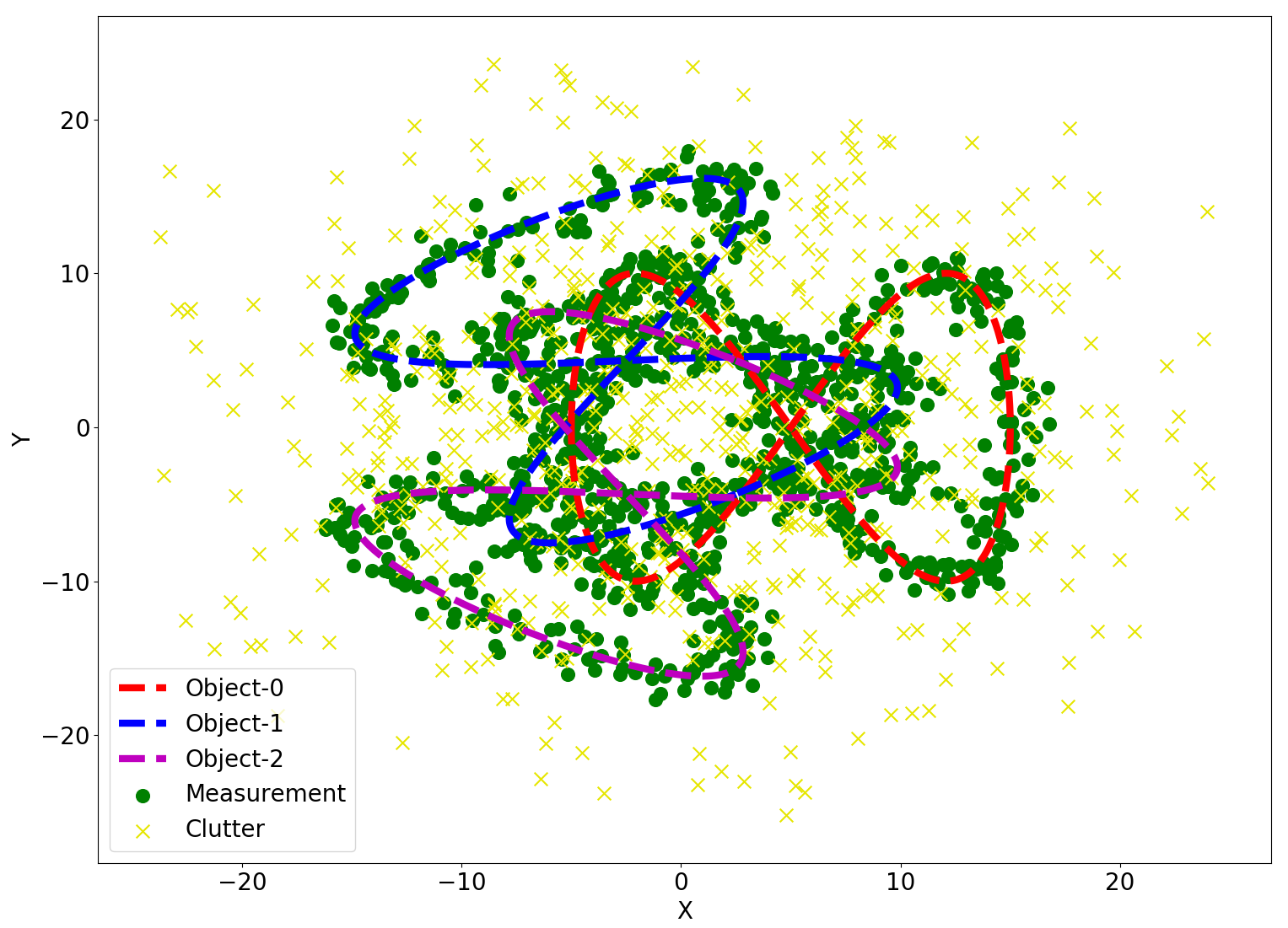
Using the same association weight computation, we compare the performance of JPDAF [2] and our PKF with 2D simulated data. In the simulation, each object is a 2D point and moves along an 8-shape trajectory. The detection probability of each object is $p^{t}_{D}=0.9$ , the measurement noise is a zero-mean Gaussian with covariance $\operatorname*{diag}(0.75,0.75)$ , and clutter is sampled uniformly in the range of $[-10,10]^{2}$ around each ground-truth point. A visualization of 3 simulated objects can be found in Figure 2.

The errors and speed of tracking 3 and 5 objects in simulation are shown in Table 1. PKF achieves lower tracking errors than JPDAF [2] implemented by [19]. Our intuition as to why PKF achieves lower errors is provided in the first paragraph of Sec. 4.3.1. The experiments also show that PKF can track at a comparable speed with JPDAF.

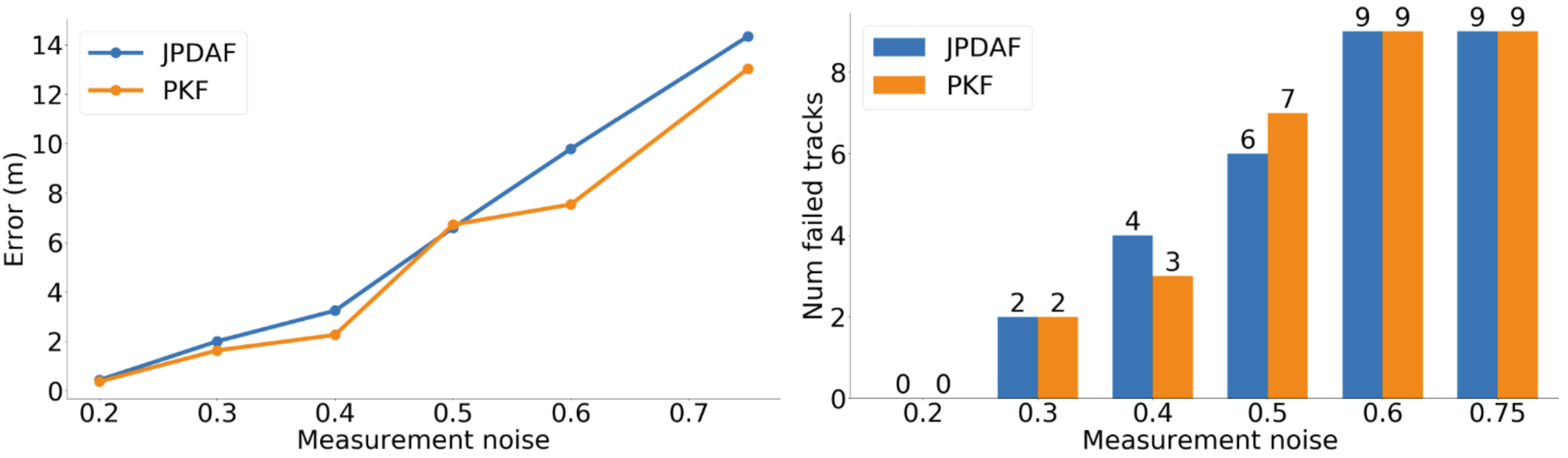
We also compare the two algorithms with a larger number of objects, i.e., 10 objects, under different levels of measurement noises. In this setting, we increase the detection probability to $0.95$ to avoid frequent tracking failures. The clutter generation remains the same and we test with measurement noises from $0.2$ to $0.75$ . The results can be found in Figure 3. We can see that our filter obtains lower tracking errors in most cases. The number of failed tracks is almost the same as JPDAF [2]. The average fps of JPDAF with 10 objects is $1284$ and that of ours is $1080$ .

Table 1: Comparison of tracking error (

l2

norm in meters) and speed (frames per second (fps)) among binary association, JPDAF [2], and PKF in simulation.

$N_{obj}$	Method	Obj 1	Obj 2	Obj 3	Obj 4	Obj 5	Avg	fps
3	Binary	2.16	1.36	1.80	-	-	1.78	5062
	JPDAF [2]	0.70	0.60	0.65	-	-	0.65	3631
	PKF	0.70	0.57	0.58	-	-	0.62	3235
5	Binary	8.37	19.36	17.34	11.37	14.53	14.20	3061
	JPDAF [2]	0.68	0.73	0.62	0.63	0.66	0.66	2567
	PKF	0.60	0.68	0.58	0.61	0.61	0.62	2172

5 Application to multi-object tracking

In this section, we apply our PKF to the MOT task.

5.1 Algorithm design

To make the filter work efficiently in practice, we introduce a hybrid data association scheme that applies probabilistic data association only to a subset of ambiguous measurements. Also, we force the state covariance matrix to be block diagonal so that each track is estimated by a separate filter, although the states are still considered jointly when evaluating the data association probabilities. We follow SORT [6] and model each object’s state as $\mathbf{x}=[u,v,s,r,\dot{u},\dot{v},\dot{s}]^{\top}$ , where $u$ and $v$ represent the horizontal and vertical pixel location of the center of the object bounding box, while $s$ and $r$ represent the scale (area) and the aspect ratio of the object’s bounding box respectively. The detections are converted into $\mathbf{z}=[u,v,s,r]^{\top}$ .

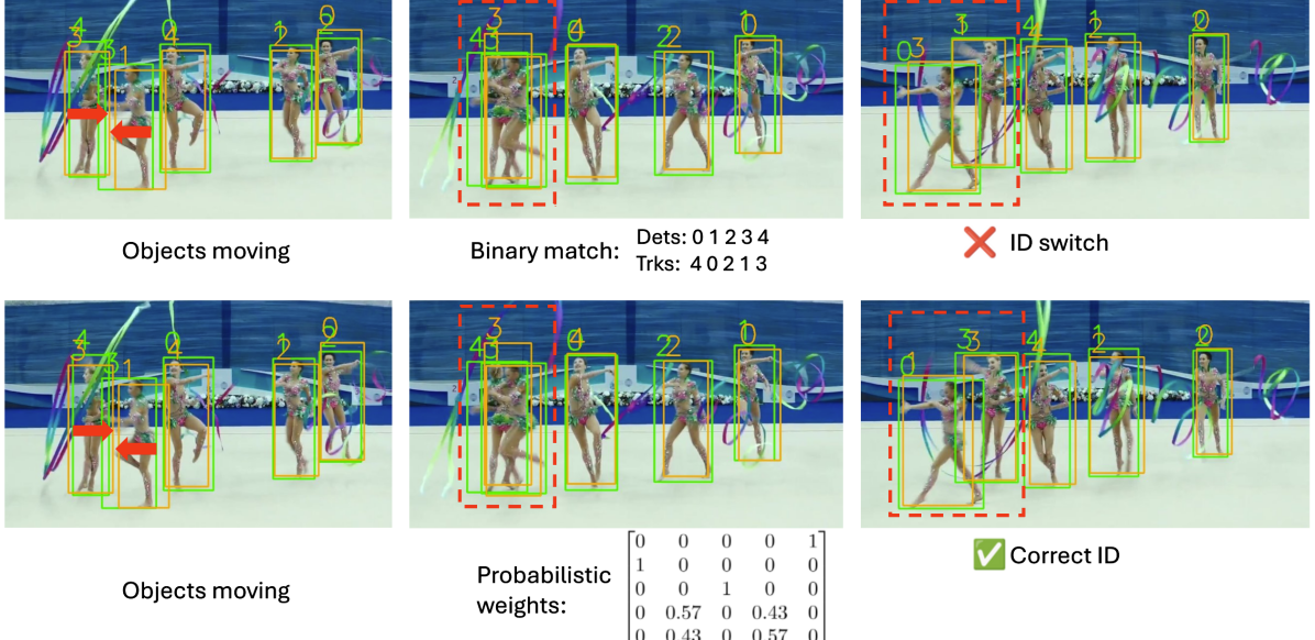
Hybrid data association Constructing a probability matrix using all measurements and states and computing the association weights according to Proposition 1 can be slow and potentially harm the tracking accuracy due to low-probability measurements. A binary matching algorithm, such as the Hungarian [23] or the Jonker-Volgenant [21], is efficient but may make incorrect hard decisions when there is ambiguity. We propose a hybrid association scheme to take advantage of both matching types. Given measurements $\mathbf{z}_{t,k}$ , $k=1,\ldots,M_{t}$ and states $\mathbf{x}_{t,j}$ , $j=1,\ldots,N$ , we first compute a score matrix $S_{t}\in\mathbb{R}^{M_{t}\times N}$ with entries $[S_{t}]_{kj}$ equal to the intersection over union (IoU) for each measurement-object bounding-box pair. A binary matching algorithm is applied to $S_{t}$ to obtain a binary matching weight matrix. Then, we perform an ambiguity check. For each row $k$ of $S_{t}$ (corresponding to measurement $\mathbf{z}_{t,k}$ ), we sort the scores from high to low. Supposing the rank is $\mathbf{x}_{t,j_{1}}\ \mathbf{x}_{t,j_{2}}\cdots\mathbf{x}_{t,j_{N}}$ , if object $\mathbf{x}_{t,j_{2}}$ has a score over a threshold $\tau_{ambig}$ , e.g., $90\%$ the score of object $\mathbf{x}_{t,j_{1}}$ , then $\mathbf{x}_{t,j_{1}}$ and $\mathbf{x}_{t,j_{2}}$ are ambiguous objects, and the measurement $\mathbf{z}_{t,k}$ is an ambiguous measurement. Then, we compare $\mathbf{x}_{t,j_{2}}$ and $\mathbf{x}_{t,j_{3}}$ and so on. We repeat this for all objects and measurements to obtain an ambiguous set. Measurements and objects with their matches marked as ambiguous will also be added to the ambiguous set. Proposition 1 is only applied to the ambiguous set of measurements and objects. Finally, we replace the elements in the initial binary matching weight matrix with the corresponding probabilistic weights. An illustration of how our proposed probabilistic data association Kalman filter benefits the ambiguous case is shown in Figure 4 where binary association causes a wrong ID switch while our proposed association can obtain a correct ID.

Each object as a single filter Instead of storing all objects in the filter state, we create a filter for each new object (which is equivalent to enforcing a block-diagonal covariance matrix). This avoids a large state covariance and observation Jacobian $\bar{H}_{t+1}$ in (17), which speeds up the tracking especially when the number of objects is large. After we get the association weight matrix $W$ , each column vector $\mathbf{w}_{j}$ corresponds to a tracked object with measurement association weights. All measurements with a weight larger than a threshold $\tau_{weight}$ are used to update the tracker by Proposition 2. The thresholding helps exclude potential outliers and achieve stable computation.

5.2 Evaluation

Datasets

We evaluate PKF on multiple MOT datasets, including MOT17 [27], MOT20 [15], and DanceTrack [40]. MOT17 and MOT20 focus on crowded pedestrian tracking in public places. DanceTrack is a dancing-scene dataset, where the objects have similar appearances, move fast, highly non-linearly, and cross over each other frequently, thus imposing a higher requirement on data association.

Metrics We use higher order tracking accuracy (HOTA) [24] as our main metric because it balances between detection accuracy and association accuracy. We also report the AssA [24] and IDF1 [38] metrics which emphasize data association accuracy and the MOTA [5] metric which emphasizes the detection accuracy.

Implementation In performing the data association ambiguity check, we compute the IoU between detections and tracked bounding boxes. To construct the matrix $Q$ in Proposition 1, we treat $UoI:=1/IoU$ as a distance (not an actual distance function mathematically) and compute the conditional probability as $p(\mathbf{z}_{t,k}|\mathbf{x}_{t,j})\propto\exp(-\alpha UoI)$ , where $\alpha$ is a scaling factor. We found $\alpha=2$ to work well in practice. On MOT17 [27] and DanceTrack [40], the ambiguity check threshold was set to $\tau_{ambig}=0.9$ . On MOT20, we set $\tau_{ambig}=0.95$ since the pedestrians are more crowded. The weight threshold was set at $\tau_{weight}=0.25$ . We used the publicly available YOLOX weights by ByteTrack [47]. Following the common practice of SORT [6], we set the detection confidence threshold at $0.4$ for MOT20 and $0.6$ for other datasets. A new track is created if a detected box has IoU lower than $0.3$ with all the tracks. All experiments were conducted on a laptop with [email protected] CPU, 16 GB RAM, and RTX 3080 GPU.

Table 2: Results on MOT17 [27] testset with private detections. We share detections with ByteTrack [47] and OC-SORT [13].

Tracker	HOTA $\uparrow$	MOTA $\uparrow$	IDF1 $\uparrow$	FP( $10^{4}$ ) $\downarrow$	FN( $10^{4}$ ) $\downarrow$	IDs $\downarrow$	Frag $\downarrow$	AssA $\uparrow$	AssR $\uparrow$
FairMOT [46]	59.3	73.7	72.3	2.75	11.7	3303	8073	58.0	63.6
QDTrack [33]	53.9	68.7	66.3	2.66	14.7	3378	8091	52.7	57.2
MOTR [45]	57.2	71.9	68.4	2.11	13.6	2115	3897	55.8	59.2
TransMOT [14]	61.7	76.7	75.1	3.62	9.32	2346	7719	59.9	66.5
MeMOT [11]	56.9	72.5	69.0	2.72	11.5	2724	-	55.2	-
OC-SORT [13]	63.2	78.0	77.5	1.51	10.8	1950	2040	63.2	67.5
ByteTrack [47]	63.1	80.3	77.3	2.55	8.37	2196	2277	62.0	68.2
PKF	63.3	78.3	77.7	1.56	10.5	2130	2754	63.4	67.4

5.3 Benchmark results

MOT17 and MOT20

The quantitative results on MOT17 [27] and MOT20 [15] are shown in Table 2 and 3. To get a fair comparison, we use the same detections as ByteTrack [47] and OC-SORT [13] and inherit the linear interpolation. While ByteTrack [47] does multiple rounds of associations and OC-SORT makes use of velocities, does object recovery, and re-updates, PKF only does one round of association using only bounding boxes and performs one single update step. We also do not use the adaptive detection thresholds as in ByteTrack [47] for generalization. We can see that our method is able to achieve comparable results with those two methods [47, 13] and is better in data association as indicated by the higher IDF1 and AssA and achieves higher HOTA results. Note that our method is compatible with techniques used by other methods, like multiple rounds of associations [47], taking into account velocities [13], and doing object recovery [13] but we did not incorporate these to keep the results clear.

Table 3: Results on MOT20 [15] testset with private detections. We share detections with ByteTrack [47] and OC-SORT [13].

Tracker	HOTA $\uparrow$	MOTA $\uparrow$	IDF1 $\uparrow$	FP( $10^{4}$ ) $\downarrow$	FN( $10^{4}$ ) $\downarrow$	IDs $\downarrow$	Frag $\downarrow$	AssA $\uparrow$	AssR $\uparrow$
FairMOT [46]	54.6	61.8	67.3	10.3	8.89	5243	7874	54.7	60.7
TransMOT [14]	61.9	77.5	75.2	3.42	8.08	1615	2421	60.1	66.3
MeMOT [11]	54.1	63.7	66.1	4.79	13.8	1938	-	55.0	-
OC-SORT [13]	62.1	75.5	75.9	1.80	10.8	913	1198	62.0	67.5
ByteTrack [47]	61.3	77.8	75.2	2.62	8.76	1223	1460	59.6	66.2
PKF	62.3	75.4	76.3	1.73	10.9	980	1584	62.7	67.6

Table 4: Results on DanceTrack [40] testset. Methods in blue share detections.

Tracker	HOTA $\uparrow$	DetA $\uparrow$	AssA $\uparrow$	MOTA $\uparrow$	IDF1 $\uparrow$
CenterTrack [49]	41.8	78.1	22.6	86.8	35.7
FairMOT [46]	39.7	66.7	23.8	82.2	40.8
QDTrack [33]	45.7	72.1	29.2	83.0	44.8
TraDes [43]	43.3	74.5	25.4	86.2	41.2
MOTR [45]	54.2	73.5	40.2	79.7	51.5
SORT [6]	47.9	72.0	31.2	91.8	50.8
DeepSORT [42]	45.6	71.0	29.7	87.8	47.9
ByteTrack [47]	47.3	71.6	31.4	89.5	52.5
OC-SORT [13]	54.5	80.4	37.1	89.4	54.0
PKF	51.7	79.8	33.5	89.1	50.1
PKF + OCM&OCR	55.4	79.5	38.7	89.2	54.9

DanceTrack The results on DanceTrack [40] are shown in Table 4. We can see that PKF achieves better results than SORT [6] and ByteTrack [47]. Since the movement is significant and the number of objects is usually fixed in a dancing scene, we find that OCM (velocity) and OCR (object recovery) proposed in OC-SORT [13] are useful. By incorporating these two components, we can further outperform OC-SORT without ORU (re-update) [13]. In this dataset, there are a lot of occlusions and the dancers can move dramatically. The increase of AssA and IDF1 shows again the advantage of PKF in terms of association. We can see that PKF obtains lower DetA than [13]. This is because the probabilistic data association can incorporate incorrect detections in the update step, making the position estimates slightly worse. However, we can still obtain higher HOTA since $\text{HOTA}_{\alpha}$ at a certain threshold $\alpha$ can be decomposed into two parts, a detection accuracy score (DetA) and an association accuracy score (AssA):

\text{HOTA}_{\alpha}=\sqrt{\text{DetA}_{\alpha}\cdot\text{AssA}_{\alpha}}.

(20)

The increased HOTA shows the increased association quality can compensate for relatively worse position updates.

Table 5: Ablation study of ambiguity check (A.C.) and weight thresholding (W.T.) on the validation sets of MOT17 [27] and DanceTrack [40] in terms of HOTA [24], IDF1 [38], and average tracking time per frame (

t

	MOT17			DanceTrack
Metrics	HOTA $\uparrow$	IDF1 $\uparrow$	$t$ (ms)	HOTA $\uparrow$	IDF1 $\uparrow$	$t$ (ms)
Binary	66.4	77.8	5.9	52.6	52.2	3.4
PKF w/o A.C.	44.9	52.8	4970.6	44.2	45.2	121.2
PKF w/o W.T.	66.6	78.1	6.3	52.0	50.4	3.8
PKF complete	66.8	78.5	6.2	53.3	53.2	3.7

Ablation study We study the effect of the ambiguity check and weight thresholding on the validation sets of MOT17 and DanceTrack. The results are shown in Table 5. We observed that associating all measurements and tracks directly not only decreases the association quality, implied by the low HOTA and IDF1, but also makes the tracking slow. Adding weight thresholding can further improve the results as low-probability measurements are usually wrong. Weight thresholding also reduces the time a bit as we use fewer measurements in the update step. The complete PKF algorithm obtains better results than binary association with almost the same tracking speed.

6 Conclusion

We derived a new formulation of the Kalman filter with probabilistic data association by formulating a variational inference problem and introducing data association as a latent variable in the EM algorithm. We showed that, in the E-step, the association probabilities can be computed as matrix permanents, while the M-step led to the usual Kalman filter prediction and update steps but with an extended measurement vector and noise covariance matrix capturing possible data associations. Our experiments demonstrated that our filter can outperform the JPDAF and can achieve top-10 results on MOT benchmarks even without using deep features. Our algorithm is not restricted to the MOT application and can serve as a general method for estimation problems with measurement ambiguity.

References

Bar-Shalom and Tse [1975] Yaakov Bar-Shalom and Edison Tse. Tracking in a cluttered environment with probabilistic data association. Automatica, 11(5):451–460, 1975.
Bar-Shalom et al. [2009] Yaakov Bar-Shalom, Fred Daum, and Jim Huang. The probabilistic data association filter. IEEE Control Systems Magazine, 29(6):82–100, 2009.
Barfoot et al. [2020] Timothy D Barfoot, James R Forbes, and David J Yoon. Exactly sparse gaussian variational inference with application to derivative-free batch nonlinear state estimation. IEEE IJRR, 39(13):1473–1502, 2020.
Bergmann et al. [2019] Philipp Bergmann, Tim Meinhardt, and Laura Leal-Taixe. Tracking without bells and whistles. In CVPR, pages 941–951, 2019.
Bernardin and Stiefelhagen [2008] Keni Bernardin and Rainer Stiefelhagen. Evaluating multiple object tracking performance: the clear mot metrics. EURASIP Journal on Image and Video Processing, 2008:1–10, 2008.
Bewley et al. [2016] Alex Bewley, Zongyuan Ge, Lionel Ott, Fabio Ramos, and Ben Upcroft. Simple online and realtime tracking. In ICIP, pages 3464–3468, 2016.
Bishop [2006] Christopher M Bishop. Pattern Recognition and Machine Learning. Springer, 2006.
Blom and Bloem [2000] Henk AP Blom and Edwin A Bloem. Probabilistic data association avoiding track coalescence. IEEE TAC, 45(2):247–259, 2000.
Bowman et al. [2017] Sean L Bowman, Nikolay Atanasov, Kostas Daniilidis, and George J Pappas. Probabilistic data association for semantic slam. In ICRA, pages 1722–1729, 2017.
Brasó and Leal-Taixé [2020] Guillem Brasó and Laura Leal-Taixé. Learning a neural solver for multiple object tracking. In CVPR, pages 6247–6257, 2020.
Cai et al. [2022] Jiarui Cai, Mingze Xu, Wei Li, Yuanjun Xiong, Wei Xia, Zhuowen Tu, and Stefano Soatto. MeMOT: Multi-object tracking with memory. In CVPR, pages 8090–8100, 2022.
Cao et al. [2024] Hanwen Cao, Sriram Shreedharan, and Nikolay Atanasov. Multi-Robot Object SLAM Using Distributed Variational Inference. IEEE Robotics and Automation Letters, 9(10):8722–8729, 2024.
Cao et al. [2023] Jinkun Cao, Jiangmiao Pang, Xinshuo Weng, Rawal Khirodkar, and Kris Kitani. Observation-centric sort: Rethinking sort for robust multi-object tracking. In CVPR, pages 9686–9696, 2023.
Chu et al. [2023] Peng Chu, Jiang Wang, Quanzeng You, Haibin Ling, and Zicheng Liu. Transmot: Spatial-temporal graph transformer for multiple object tracking. In WACV, pages 4870–4880, 2023.
Dendorfer et al. [2020] Patrick Dendorfer, Hamid Rezatofighi, Anton Milan, Javen Shi, Daniel Cremers, Ian Reid, Stefan Roth, Konrad Schindler, and Laura Leal-Taixé. MOT20: A benchmark for multi object tracking in crowded scenes. arXiv preprint arXiv:2003.09003, 2020.
Doherty et al. [2019] Kevin Doherty, Dehann Fourie, and John Leonard. Multimodal semantic slam with probabilistic data association. In ICRA, pages 2419–2425, 2019.
Feichtenhofer et al. [2017] Christoph Feichtenhofer, Axel Pinz, and Andrew Zisserman. Detect to track and track to detect. In ICCV, pages 3038–3046, 2017.
Godinez and Rohr [2014] William J Godinez and Karl Rohr. Tracking multiple particles in fluorescence time-lapse microscopy images via probabilistic data association. IEEE transactions on medical imaging, 34(2):415–432, 2014.
Hiscocks et al. [2023] Steven Hiscocks, Jordi Barr, Nicola Perree, James Wright, Henry Pritchett, Oliver Rosoman, Michael Harris, Roisín Gorman, Sam Pike, Peter Carniglia, Lyudmil Vladimirov, and Benedict Oakes. Stone Soup: No longer just an appetiser. In International Conference on Information Fusion (FUSION), 2023.
Huber and Law [2008] Mark Huber and Jenny Law. Fast approximation of the permanent for very dense problems. In Proceedings of the nineteenth annual ACM-SIAM symposium on Discrete algorithms, pages 681–689, 2008.
Jonker and Volgenant [1988] Roy Jonker and Ton Volgenant. A shortest augmenting path algorithm for dense and sparse linear assignment problems. In DGOR/NSOR: Papers of the 16th Annual Meeting of DGOR in Cooperation with NSOR/Vorträge der 16. Jahrestagung der DGOR zusammen mit der NSOR, pages 622–622, 1988.
Kaess et al. [2008] Michael Kaess, Ananth Ranganathan, and Frank Dellaert. isam: Incremental smoothing and mapping. IEEE TRO, 24(6):1365–1378, 2008.
Kuhn [1955] Harold W Kuhn. The hungarian method for the assignment problem. Naval research logistics quarterly, 2(1-2):83–97, 1955.
Luiten et al. [2021] Jonathon Luiten, Aljosa Osep, Patrick Dendorfer, Philip Torr, Andreas Geiger, Laura Leal-Taixé, and Bastian Leibe. Hota: A higher order metric for evaluating multi-object tracking. IJCV, 129:548–578, 2021.
Meinhardt et al. [2022] Tim Meinhardt, Alexander Kirillov, Laura Leal-Taixe, and Christoph Feichtenhofer. Trackformer: Multi-object tracking with transformers. In CVPR, pages 8844–8854, 2022.
Meyer et al. [2018] Florian Meyer, Thomas Kropfreiter, Jason L Williams, Roslyn Lau, Franz Hlawatsch, Paolo Braca, and Moe Z Win. Message passing algorithms for scalable multitarget tracking. Proceedings of the IEEE, 106(2):221–259, 2018.
Milan et al. [2016] Anton Milan, Laura Leal-Taixé, Ian Reid, Stefan Roth, and Konrad Schindler. MOT16: A benchmark for multi-object tracking. arXiv preprint arXiv:1603.00831, 2016.
Montella [2011] Corey Montella. The kalman filter and related algorithms: A literature review. Res. Gate, pages 1–17, 2011.
Musicki and Evans [2004] Darko Musicki and Robin Evans. Joint integrated probabilistic data association: Jipda. IEEE transactions on Aerospace and Electronic Systems, 40(3):1093–1099, 2004.
Musicki et al. [1994] Darko Musicki, Robin Evans, and Srdjan Stankovic. Integrated probabilistic data association. IEEE TAC, 39(6):1237–1241, 1994.
Neira and Tardós [2001] José Neira and Juan D Tardós. Data association in stochastic mapping using the joint compatibility test. IEEE Transactions on robotics and automation, 17(6):890–897, 2001.
Nijenhuis and Wilf [2014] Albert Nijenhuis and Herbert S Wilf. Combinatorial algorithms: for computers and calculators. Elsevier, 2014.
Pang et al. [2021] Jiangmiao Pang, Linlu Qiu, Xia Li, Haofeng Chen, Qi Li, Trevor Darrell, and Fisher Yu. Quasi-dense similarity learning for multiple object tracking. In CVPR, pages 164–173, 2021.
Rakai et al. [2022] Lionel Rakai, Huansheng Song, ShiJie Sun, Wentao Zhang, and Yanni Yang. Data association in multiple object tracking: A survey of recent techniques. Expert systems with applications, 192:116300, 2022.
Redmon et al. [2016] Joseph Redmon, Santosh Divvala, Ross Girshick, and Ali Farhadi. You only look once: Unified, real-time object detection. In NeurIPS, pages 779–788, 2016.
Ren et al. [2015] Shaoqing Ren, Kaiming He, Ross Girshick, and Jian Sun. Faster r-cnn: Towards real-time object detection with region proposal networks. NeurIPS, 28, 2015.
Rezatofighi et al. [2015] Seyed Hamid Rezatofighi, Anton Milan, Zhen Zhang, Qinfeng Shi, Anthony Dick, and Ian Reid. Joint probabilistic data association revisited. In ICCV, pages 3047–3055, 2015.
Ristani et al. [2016] Ergys Ristani, Francesco Solera, Roger Zou, Rita Cucchiara, and Carlo Tomasi. Performance measures and a data set for multi-target, multi-camera tracking. In ECCV, pages 17–35. Springer, 2016.
Stein [1981] Charles M Stein. Estimation of the mean of a multivariate normal distribution. The Annals of Statistics, pages 1135–1151, 1981.
Sun et al. [2022] Peize Sun, Jinkun Cao, Yi Jiang, Zehuan Yuan, Song Bai, Kris Kitani, and Ping Luo. Dancetrack: Multi-object tracking in uniform appearance and diverse motion. In CVPR, pages 20993–21002, 2022.
Vaswani et al. [2017] Ashish Vaswani, Noam Shazeer, Niki Parmar, Jakob Uszkoreit, Llion Jones, Aidan N Gomez, Łukasz Kaiser, and Illia Polosukhin. Attention is all you need. NeurIPS, 30, 2017.
Wojke et al. [2017] Nicolai Wojke, Alex Bewley, and Dietrich Paulus. Simple online and realtime tracking with a deep association metric. In ICIP, pages 3645–3649, 2017.
Wu et al. [2021] Jialian Wu, Jiale Cao, Liangchen Song, Yu Wang, Ming Yang, and Junsong Yuan. Track to detect and segment: An online multi-object tracker. In CVPR, pages 12352–12361, 2021.
Yang et al. [2018] Shishan Yang, Kolja Thormann, and Marcus Baum. Linear-time joint probabilistic data association for multiple extended object tracking. In IEEE Sensor Array and Multichannel Signal Processing Workshop (SAM), pages 6–10, 2018.
Zeng et al. [2022] Fangao Zeng, Bin Dong, Yuang Zhang, Tiancai Wang, Xiangyu Zhang, and Yichen Wei. MOTR: End-to-end multiple-object tracking with transformer. In ECCV, pages 659–675. Springer, 2022.
Zhang et al. [2021] Yifu Zhang, Chunyu Wang, Xinggang Wang, Wenjun Zeng, and Wenyu Liu. Fairmot: On the fairness of detection and re-identification in multiple object tracking. IJCV, 129:3069–3087, 2021.
Zhang et al. [2022] Yifu Zhang, Peize Sun, Yi Jiang, Dongdong Yu, Fucheng Weng, Zehuan Yuan, Ping Luo, Wenyu Liu, and Xinggang Wang. Bytetrack: Multi-object tracking by associating every detection box. In ECCV, pages 1–21. Springer, 2022.
Zhou et al. [2019] Xingyi Zhou, Dequan Wang, and Philipp Krähenbühl. Objects as points. arXiv preprint arXiv:1904.07850, 2019.
Zhou et al. [2020] Xingyi Zhou, Vladlen Koltun, and Philipp Krähenbühl. Tracking objects as points. In ECCV, pages 474–490. Springer, 2020.

\thetitle

Supplementary Material

7 Proof of Proposition 1

Define sets $\mathcal{K}^{-k}_{t}:=\{1,...,M_{t}\}\backslash\{k\}$ , $\mathcal{J}^{-j}:=\{1,...,N\}\backslash\{j\}$ , and a function $\bar{\delta}_{t}:\mathcal{K}^{-k}_{t}\rightarrow\mathcal{J}^{-j}$ . Then, (6) can be rewritten as:

$\displaystyle w^{t}_{k,j}$	$\displaystyle\propto\!\!\!\!\sum_{\delta\in\mathcal{D}_{t}(k,j)}\prod_{k^{\prime}=1}^{M_{t}}p\left(\mathbf{z}_{t,k^{\prime}}\|\delta_{t}(k^{\prime})\right)$
	$\displaystyle=\sum_{\bar{\delta}_{t}}p(\mathbf{z}_{k}\|\delta_{t}(k)=j)\prod_{\bar{k}\in\mathcal{K}^{-k}_{t}}p\left(\mathbf{z}_{t,\bar{k}}\|\bar{\delta}_{t}(\bar{k})\right)$
	$\displaystyle=p(\mathbf{z}_{k}\|\delta_{t}(k)=j)\sum_{\bar{\delta}_{t}}\prod_{\bar{k}\in\mathcal{K}^{-k}_{t}}p(\mathbf{z}_{t,\bar{k}}\|\bar{\delta}_{t}(\bar{k}))$
	$\displaystyle=Q^{t}(k,j)\operatorname*{per}(Q^{t}_{-kj}),$	(21)

where the derivation in the last line follows by the definition of the matrix permanent in (7).

8 Proof of Proposition 2

In this section, we show how optimizing (12) leads to Proposition 2. The objective function $f^{(i)}(q)$ in (12) can be rewritten as:

$\displaystyle f^{(i)}(q)\!=$	$\displaystyle\mathbb{E}_{\delta_{t+1}}\mathbb{E}_{\bar{\mathbf{x}}^{(i)}}\!\!\left\{\mathbb{E}_{q}\!\!\left[\!\log p(\bar{\mathbf{x}},\mathbf{z}_{t+1},\mathbf{u}_{t},\delta_{t+1})\|\bar{\mathbf{x}}^{(i)},\mathbf{z}_{t+1}\!\right]\!\right\}$
	$\displaystyle-\mathbb{E}_{\delta_{t+1}}\mathbb{E}_{\bar{\mathbf{x}}^{(i)}}\left\{\mathbb{E}_{q}\left[\log q\right]\right\}$
$\displaystyle=$	$\displaystyle\mathbb{E}_{q}\!\!\left\{\!\mathbb{E}_{\delta_{t+1}}\!\mathbb{E}_{\bar{\mathbf{x}}^{(i)}}\!\!\left[\!\log p(\bar{\mathbf{x}},\mathbf{z}_{t+1},\mathbf{u}_{t},\delta_{t+1})\|\bar{\mathbf{x}}^{(i)},\mathbf{z}_{t+1}\!\right]\!\right\}$
	$\displaystyle\underbrace{-\mathbb{E}_{q}\left[\log q\right]}_{\text{entropy}}$
$\displaystyle=$	$\displaystyle\mathbb{E}_{q}\left[J(\bar{\mathbf{x}})\right]\underbrace{-\frac{1}{2}\log\left(\|\Sigma^{-1}\|\right)+c}_{\text{entropy}},$	(22)

where $c$ is some constant unrelated to $q$ . To find the maximizer of (12), we take the gradient of $f(q)$ w.r.t. $\boldsymbol{\mu}$ and $\Sigma$ of $q$ :

$\displaystyle\frac{\partial f}{\partial\boldsymbol{\mu}^{\top}}$	$\displaystyle=\Sigma^{-1}\mathbb{E}_{q}\left[(\bar{\mathbf{x}}-\boldsymbol{\mu})J(\bar{\mathbf{x}})\right]$	(23)
$\displaystyle\frac{\partial^{2}f}{\partial\boldsymbol{\mu}^{\top}\partial\boldsymbol{\mu}}$	$\displaystyle=\Sigma^{-1}\mathbb{E}_{q}\left[(\bar{\mathbf{x}}-\boldsymbol{\mu})(\bar{\mathbf{x}}-\boldsymbol{\mu})^{\top}J(\bar{\mathbf{x}})\right]\Sigma^{-1}$
	$\displaystyle-\Sigma^{-1}\mathbb{E}_{q}\left[J(\bar{\mathbf{x}})\right]$	(24)
$\displaystyle\frac{\partial f}{\partial\Sigma^{-1}}$	$\displaystyle=-\frac{1}{2}\mathbb{E}_{q}\left[(\bar{\mathbf{x}}-\boldsymbol{\mu})(\bar{\mathbf{x}}-\boldsymbol{\mu})^{\top}J(\bar{\mathbf{x}})\right]$
	$\displaystyle+\frac{1}{2}\Sigma\mathbb{E}_{q}[J(\bar{\mathbf{x}})]-\frac{1}{2}\Sigma$	(25)

Using (24) and (25), we get the following relationship:

\frac{\partial^{2}f}{\partial\boldsymbol{\mu}^{\top}\partial\boldsymbol{\mu}}=-\Sigma^{-1}-2\Sigma^{-1}\frac{\partial f}{\partial\Sigma^{-1}}\Sigma^{-1}.

(26)

To compute the above derivatives, we use of Stein’s Lemma [39]. With our notation, the Lemma says:

\mathbb{E}_{q}[(\bar{\mathbf{x}}-\boldsymbol{\mu})J(\bar{\mathbf{x}})]=\Sigma\mathbb{E}_{q}\left[\frac{\partial J}{\partial\bar{\mathbf{x}}}\right].

(27)

To compute $\frac{\partial J}{\partial\bar{\mathbf{x}}}$ , we first analyze the term $J(\bar{\mathbf{x}})$ :

$\displaystyle J(\bar{\mathbf{x}})\!$	$\displaystyle=\!\mathbb{E}_{\delta_{t+1}}\!\mathbb{E}_{\bar{\mathbf{x}}^{(i)}}\!\!\left[\!\log p(\bar{\mathbf{x}},\mathbf{z}_{t+1},\mathbf{u}_{t},\delta_{t+1})\|\bar{\mathbf{x}}^{(i)}\!,\mathbf{z}_{t+1}\!\right]$	(28)
	$\displaystyle=\!\!\sum_{\delta\in\mathcal{D}_{t+1}}\!\!\!\mathbb{E}_{\bar{\mathbf{x}}^{(i)}}\left[p(\delta\|\bar{\mathbf{x}}^{(i)},\mathbf{z}_{t+1})\right]\log p(\bar{\mathbf{x}},\mathbf{z}_{t+1},\mathbf{u}_{t},\delta)$
	$\displaystyle\propto\!\!\sum_{\delta\in\mathcal{D}_{t+1}}\!\!\!p(\delta\|\mathbf{z}_{t+1})\log(p(\mathbf{z}_{t+1}\|\bar{\mathbf{x}},\delta)p(\bar{\mathbf{x}}\|\mathbf{u}_{t}))$
	$\displaystyle=\!\!\underbrace{\sum_{\delta\in\mathcal{D}_{t+1}}\!\!\!p(\delta\|\mathbf{z}_{t+1})\log p(\mathbf{z}_{t+1}\|\bar{\mathbf{x}},\delta)}_{J_{\mathbf{z}_{t+1}}(\bar{\mathbf{x}})}+\underbrace{\vphantom{\sum_{\delta\in\mathcal{D}_{t+1}}}\log p(\bar{\mathbf{x}}\|\mathbf{u}_{t})}_{J_{\mathbf{u}_{t}}(\bar{\mathbf{x}})}.$

Focusing on the first term on the right, we get:

$\displaystyle J_{\mathbf{z}_{t+1}}$	$\displaystyle(\bar{\mathbf{x}})=\sum_{\delta\in\mathcal{D}_{t+1}}p(\delta\|\mathbf{z}_{t+1})\log p(\mathbf{z}_{t+1}\|\mathbf{x}_{t+1},\delta)$	(29)
	$\displaystyle=\!\sum_{k=1}^{M_{t}}\sum_{\delta\in\mathcal{D}_{t+1}}\!\!\!p(\delta\|\mathbf{z}_{t+1})\log p(\mathbf{z}_{t+1,k}\|\mathbf{x}_{t+1,\delta(k)})$
	$\displaystyle=\!\sum_{k=1}^{M_{t}}\!\sum_{j=1}^{N}\sum_{\delta\in\mathcal{D}_{t+1}(k,j)}\!\!\!\!\!\!\!\!\!p(\delta\|\mathbf{z}_{t+1})\!\log p(\mathbf{z}_{t+1,k}\|\mathbf{x}_{t+1,j}),$

where $\mathcal{D}_{t+1}(k,j)$ is the subset of all possible data associations that assign measurement $\mathbf{z}_{t+1,k}$ to variable $\mathbf{x}_{t+1,j}$ . Let $w^{t+1}_{k,j}\triangleq\sum_{\delta\in\mathcal{D}_{t+1}(k,j)}p(\delta|\mathbf{z}_{t+1})$ , which is the same as (6). The above equation can be rewritten as:

$\displaystyle J_{\mathbf{z}_{t+1}}(\bar{\mathbf{x}})$	$\displaystyle=\sum_{k=1}^{M_{t}}\sum_{j=1}^{N}w^{t+1}_{k,j}\log(\mathbf{z}_{t+1,k}\|\mathbf{x}_{t+1,j})$	(30)
	$\displaystyle\propto\sum_{k=1}^{M_{t}}\sum_{j=1}^{N}w^{t+1}_{k,j}(-\frac{1}{2}\\|\mathbf{z}_{t+1,k}-H\mathbf{x}_{t+1,j}\\|_{V})$
	$\displaystyle=\sum_{k=1}^{M_{t}}\sum_{j=1}^{N}-\frac{1}{2}\\|\mathbf{z}_{t+1,k}-H\mathbf{x}_{t+1,j}\\|_{V/w^{t+1}_{k,j}}^{2}.$

Then, we analyze the second term of (28):

$\displaystyle J_{\mathbf{u}_{t}}(\bar{\mathbf{x}})$	$\displaystyle=\log p(\bar{\mathbf{x}}\|\mathbf{u}_{t})$	(31)
	$\displaystyle=\log p(\mathbf{x}_{t})p(\mathbf{x}_{t+1}\|\mathbf{x}_{t},\mathbf{u}_{t})$
	$\displaystyle=\log p(\mathbf{x}_{t})+\log p(\mathbf{x}_{t+1}\|\mathbf{x}_{t},\mathbf{u}_{t})$
	$\displaystyle\propto-\frac{1}{2}\\|\mathbf{x}_{t}-\boldsymbol{\mu}_{t}\\|^{2}_{\Sigma_{t}}-\frac{1}{2}\\|\mathbf{x}_{t+1}-F\mathbf{x}_{t}-G\mathbf{u}_{t}\\|^{2}_{W}.$

Combining (30) and (31), (28) can be expanded as:

	$\displaystyle J(\bar{\mathbf{x}})\propto$	$\displaystyle\sum_{k=1}^{M_{t}}\sum_{j=1}^{N}-\frac{1}{2}\\|\mathbf{z}_{t+1,k}-H\mathbf{x}_{t+1,j}\\|_{V/w^{t+1}_{k,j}}^{2}$		(32)
		$\displaystyle-\frac{1}{2}\\|\mathbf{x}_{t}-\boldsymbol{\mu}_{t}\\|^{2}_{\Sigma_{t}}-\frac{1}{2}\\|\mathbf{x}_{t+1}-F\mathbf{x}_{t}-G\mathbf{u}_{t}\\|^{2}_{W}.$

To further simplify the objective, we stack all the known data into a lifted column $\mathbf{y}$ as

\mathbf{y}=\begin{bmatrix}\boldsymbol{\mu}_{t}\\ G\mathbf{u}_{t}\\ \bar{\mathbf{z}}_{t+1}\\ \end{bmatrix},

(33)

where $\bar{\mathbf{z}}_{t+1}$ is an expanded measurement defined as:

\bar{\mathbf{z}}_{t+1}=(I_{M_{t+1}}\otimes\mathbf{1}_{N}\otimes I_{m})\mathbf{z}_{t+1}=\begin{bmatrix}\mathbf{z}_{t+1,1}\\ \vdots\\ \mathbf{z}_{t+1,1}\\ \vdots\\ \mathbf{z}_{t+1,M_{t+1}}\\ \vdots\\ \mathbf{z}_{t+1,M_{t+1}}\end{bmatrix}\!\!\!\in\mathbb{R}^{mM_{t+1}N}

(34)

where $\mathbf{z}_{t+1,k}\in\mathbb{R}^{m}$ for all $k$ , $M_{t+1}$ is the number of measurements at time $t+1$ , and $N$ is the number of states. Define the following expanded measurement model:

\bar{\mathbf{z}}_{t+1}=\bar{H}_{t+1}\mathbf{x}_{t+1}+\bar{\mathbf{v}}_{t+1},\quad\bar{\mathbf{v}}_{t+1}\sim\mathcal{N}(\mathbf{0},\bar{V}_{t+1}),

(35)

where $\bar{V}_{t+1}$ is defined in (14) (changing $t$ to $t+1$ ) and $\bar{H}_{t+1}$ is defined as below

\bar{H}_{t+1}\!=\!\mathbf{1}_{M_{t+1}}\otimes\mathbf{I}_{N}\otimes H\!=\!\begin{bmatrix}H&\ &\ \\ \ &\ddots&\ \\ \ &\ &H\\ \ &\vdots&\ \\ H&\ &\ \\ \ &\ddots&\ \\ \ &\ &H\\ \end{bmatrix}\in\mathbb{R}^{mM_{t+1}N\times nN}.

(36)

We, then, define the following block-matrix quantities:

A=\begin{bmatrix}I&\mathbf{0}\\ -F&I\\ \mathbf{0}&\bar{H}_{t+1}\\ \end{bmatrix},\ R=\begin{bmatrix}\Sigma_{t}&\mathbf{0}&\mathbf{0}\\ \mathbf{0}&W&\mathbf{0}\\ \mathbf{0}&\mathbf{0}&\bar{V}_{t+1}\\ \end{bmatrix}.

(37)

Then, (32) can be written in a matrix form as follows:

J(\bar{\mathbf{x}})=-\frac{1}{2}(\mathbf{y}-A\bar{\mathbf{x}})^{T}R^{-1}(\mathbf{y}-A\bar{\mathbf{x}}).

(38)

The derivative $\frac{\partial J}{\partial\bar{\mathbf{x}}}$ is then

\frac{\partial J(\bar{\mathbf{x}})}{\partial\bar{\mathbf{x}}}=A^{\top}R^{-1}(\mathbf{y}-A\bar{\mathbf{x}}).

(39)

Using Stein’s Lemma (27) and (39), the first-order derivative $\frac{\partial f}{\partial\boldsymbol{\mu}^{\top}}$ (23) becomes

\frac{\partial f}{\partial\boldsymbol{\mu}^{\top}}=\mathbb{E}_{q}\left[\frac{\partial J}{\partial\bar{\mathbf{x}}}\right]=-A^{\top}R^{-1}(\mathbf{y}-A\boldsymbol{\mu}).

(40)

The second-order derivative $\frac{\partial^{2}f}{\partial\boldsymbol{\mu}^{\top}\boldsymbol{\mu}}$ is then

\frac{\partial^{2}f}{\partial\boldsymbol{\mu}^{\top}\boldsymbol{\mu}}=-A^{\top}R^{-1}A.

(41)

To get the $\Sigma$ minimizer, by setting $\frac{\partial f}{\partial\Sigma^{-1}}=0$ and using (26), we get

	$\displaystyle\Sigma^{-1}=$	$\displaystyle-\frac{\partial^{2}f}{\partial\boldsymbol{\mu}^{\top}\boldsymbol{\mu}}$		(42)
	$\displaystyle=$	$\displaystyle\begin{bmatrix}\Sigma^{-1}_{t}+F^{\top}W^{-1}F&-F^{\top}W^{-1}\\ -W^{-1}F&\bar{H}_{t+1}^{\top}\bar{V}_{t+1}^{-1}\bar{H}_{t+1}+W^{-1}\end{bmatrix}.$

Since we want to obtain the marginal distribution $q(\mathbf{x}_{t+1})$ , we need the bottom right block of the inverse of the above matrix. We make use of the following two Lemmas.

Lemma 1.

Let $S$ be a $2\times 2$ block matrix,

S=\begin{bmatrix}A&C\\ C^{\top}&B\end{bmatrix}.

(43)

If $A$ and $B$ are invertible, the inverse of $S$ is

	$\displaystyle S^{-1}=$		(44)
	$\displaystyle\begin{bmatrix}(A\!-\!CB^{-1}C^{\top})^{-1}&-A^{-1}C(B\!-\!C^{\top}\!\!A^{-1}C)^{-1}\\ -(B\!-\!C^{\top}\!\!A^{-1}C)^{-1}C^{\top}\!\!A^{-1}&(B\!-\!C^{\top}\!\!A^{-1}C)^{-1}\end{bmatrix}.$

Lemma 2.

Given matrices $A\in\mathbb{R}^{N\times N}$ , $B\in\mathbb{R}^{M\times M}$ , $C\in\mathbb{R}^{N\times M}$ , the inverse of $B+C^{\top}A^{-1}C$ is:

	$\displaystyle(B+$	$\displaystyle C^{\top}A^{-1}C)^{-1}=$		(45)
		$\displaystyle B^{-1}-B^{-1}C^{\top}(A+CB^{-1}C^{\top})^{-1}CB^{-1}.$		(45)

Using Lemma 1 and (42), we get

	$\displaystyle\Sigma^{-1}_{t+1}=$	$\displaystyle\bar{H}_{t+1}^{\top}\bar{V}_{t+1}^{-1}\bar{H}_{t+1}+W^{-1}$		(46)
		$\displaystyle-W^{-1}F(\Sigma^{-1}_{t}+F^{\top}W^{-1}F)^{-1}F^{\top}W^{-1}.$

Then, using Lemma 2, we get

	$\displaystyle\Sigma^{-1}_{t+1}$	$\displaystyle=(\Sigma^{+}_{t+1})^{-1}+\bar{H}_{t+1}^{\top}\bar{V}_{t+1}^{-1}\bar{H}_{t+1},$		(47)
	$\displaystyle\Sigma^{+}_{t+1}$	$\displaystyle=F\Sigma_{t}F^{\top}+W,$		(48)

where $\Sigma^{+}_{t+1}$ is the predicted covariance. Setting $\frac{\partial f}{\partial\boldsymbol{\mu}^{\top}}=0$ in (40), we have

	$\displaystyle\begin{bmatrix}\Sigma^{-1}_{t}+F^{\top}W^{-1}F&-F^{\top}W^{-1}\\ -W^{-1}F&W^{-1}+\bar{H}_{t+1}^{\top}\bar{V}_{t+1}^{-1}\bar{H}_{t+1}\end{bmatrix}\begin{bmatrix}\boldsymbol{\mu}^{\prime}_{t}\\ \boldsymbol{\mu}_{t+1}\end{bmatrix}$			(49)
	$\displaystyle=\begin{bmatrix}\Sigma_{t}^{-1}\boldsymbol{\mu}_{t}-F^{\top}W^{-1}G\mathbf{u}_{t}\\ W^{-1}G\mathbf{u}_{t}+\bar{H}_{t+1}^{\top}\bar{V}_{t+1}^{-1}\bar{\mathbf{z}}_{t+1}\end{bmatrix}$	.		(49)

Note that $\boldsymbol{\mu}^{\prime}_{t}$ is the mean of $\mathbf{s}_{t}$ conditioned a future measurement $\bar{\mathbf{z}}_{t+1}$ , which is not suitable to compute in online filtering. We marginalize it by left-multiplying both sides by

D=\begin{bmatrix}I&\mathbf{0}\\ W^{-1}F(\Sigma_{t}^{-1}+F^{\top}W^{-1}F)^{-1}&I\end{bmatrix}.

(50)

The simplified result is

	$\displaystyle\begin{bmatrix}\Sigma_{t}^{-1}+F^{\top}W^{-1}F&-F^{\top}W^{-1}\\ \mathbf{0}&\underline{(\Sigma^{+}_{t+1})^{-1}+\bar{H}_{t+1}^{\top}\bar{V}_{t+1}^{-1}\bar{H}_{t+1}}\end{bmatrix}\begin{bmatrix}\boldsymbol{\mu}^{\prime}_{t}\\ \boldsymbol{\mu}_{t+1}\end{bmatrix}$			(51)
	$\displaystyle=\begin{bmatrix}\Sigma^{-1}_{t}\boldsymbol{\mu}_{t}-F^{\top}W^{-1}G\mathbf{u}_{t}\\ \uwave{(\Sigma^{+}_{t+1})^{-1}(F\boldsymbol{\mu}_{t}+G\mathbf{u}_{t})+\bar{H}^{\top}_{t+1}\bar{V}_{t+1}^{-1}\bar{\mathbf{z}}_{t+1}}\end{bmatrix}$	.		(51)

While other terms are straightforward to compute, we provide explanation for the two terms marked as $\underline{(\cdot)}$ and $\uwave{(\cdot)}$ . The term $\underline{(\cdot)}$ can be obtained in the same way as (46), (47), (48). Then, let us focus on the $\uwave{(\cdot)}$ term, which is the second block of $DA^{\top}R^{-1}\mathbf{y}$ , denoted as $[DA^{\top}R^{-1}\mathbf{y}]_{2}$ . We have

	$\displaystyle[DA^{\top}R^{-1}\mathbf{y}]_{2}=W^{-1}F(\Sigma_{t}^{-1}+F^{\top}W^{-1}F)^{-1}\Sigma^{-1}_{t}\boldsymbol{\mu}$
	$\displaystyle\quad+(W^{-1}+-W^{-1}F(\Sigma_{t}^{-1}+F^{\top}W^{-1}F)F^{\top}W^{-1})G\mathbf{u}_{t}$
	$\displaystyle\quad+\bar{H}^{\top}_{t+1}\bar{V}_{t+1}^{-1}\bar{\mathbf{z}}_{t+1}.$		(52)

The second term in (52) can be simplified in the same way as (46), (47), (48) into $(\Sigma_{t+1}^{+})^{-1}G\mathbf{u}_{t}$ . The first term in (52) can be written as

	$\displaystyle\quad W^{-1}F(\Sigma_{t}^{-1}+F^{\top}W^{-1}F)^{-1}\Sigma^{-1}_{t}\boldsymbol{\mu}$
	$\displaystyle=W^{-1}F[\Sigma_{t}-\Sigma_{t}F^{\top}(W+F\Sigma_{t}F^{\top})^{-1}F\Sigma_{t}]\Sigma_{t}^{-1}\boldsymbol{\mu}_{t}$
	$\displaystyle=W^{-1}F[\Sigma_{t}-\Sigma_{t}F^{\top}(\Sigma^{+}_{t+1})^{-1}F\Sigma_{t}]\Sigma_{t}^{-1}\boldsymbol{\mu}_{t}$
	$\displaystyle=[W^{-1}-W^{-1}F\Sigma_{t}F^{\top}(\Sigma^{+}_{t+1})^{-1}]F\boldsymbol{\mu}_{t}$
	$\displaystyle=[W^{-1}-W^{-1}(\Sigma^{+}_{t+1}-W)(\Sigma^{+}_{t+1})^{-1}]F\boldsymbol{\mu}_{t}$
	$\displaystyle=(\Sigma^{+}_{t+1})^{-1}F\boldsymbol{\mu}_{t}.$		(53)

This way, (52) is simplified to the $\uwave{(\cdot)}$ term in (51).

The term $\boldsymbol{\mu}^{+}_{t+1}=F\boldsymbol{\mu}_{t}+G\mathbf{u}_{t}$ is the predicted mean. Bringing all of the above together, we have the recursive filtering as follows:


$\displaystyle\text{Predictor}:$
$\displaystyle\quad\Sigma^{+}_{t+1}$	$\displaystyle=F\Sigma_{t}F^{\top}+W,$	(54a)
$\displaystyle\boldsymbol{\mu}^{+}_{t+1}$	$\displaystyle=F\boldsymbol{\mu}_{t}+G\mathbf{u}_{t}.$	(54b)
$\displaystyle\text{Corrector}:$
$\displaystyle\quad\Sigma_{t+1}^{-1}$	$\displaystyle=(\Sigma^{+}_{t+1})^{-1}+\bar{H}_{t+1}^{\top}\bar{V}_{t+1}^{-1}\bar{H}_{t+1},$	(54c)
$\displaystyle\Sigma_{t+1}^{-1}\boldsymbol{\mu}_{t+1}$	$\displaystyle=(\Sigma^{+}_{t+1})^{-1}\boldsymbol{\mu}^{+}_{t+1}+\bar{H}_{t+1}^{T}\bar{V}_{t+1}^{-1}\bar{\mathbf{z}}_{t+1}.$	(54d)

To obtain the canonical form, we first define the Kalman gain $\bar{K}_{t+1}$ as

\bar{K}_{t+1}=\Sigma_{t+1}\bar{H}_{t+1}^{\top}\bar{V}_{t+1}^{-1},

(55)

then we do the following manipulation:

$\displaystyle I$	$\displaystyle=\Sigma_{t+1}\left[(\Sigma_{t+1}^{+})^{-1}+\bar{H}_{t+1}^{\top}\bar{V}_{t+1}^{-1}\bar{H}_{t+1}\right]$	(56)
$\displaystyle I$	$\displaystyle=\Sigma_{t+1}(\Sigma_{t+1}^{+})^{-1}+\bar{K}_{t+1}\bar{H}_{t+1}$
$\displaystyle\Sigma_{t+1}$	$\displaystyle=(I-\bar{K}_{t+1}\bar{H}_{t+1})\Sigma_{t+1}^{+}$
$\displaystyle\bar{K}_{t+1}\bar{V}_{t+1}$	$\displaystyle=(I-\bar{K}_{t+1}\bar{H}_{t+1})\Sigma_{t+1}^{+}\bar{H}_{t+1}^{\top}.$

Thus, we obtain the canonical Kalman gain

\bar{K}_{t+1}=\Sigma^{+}_{t+1}\bar{H}_{t+1}^{\top}(\bar{H}_{t+1}\Sigma^{+}_{t+1}\bar{H}_{t+1}^{\top}+\bar{V}_{t+1})^{-1},

(57)

and rewrite the recursive filter in canonical form:


predictor:
$\displaystyle\quad\boldsymbol{\mu}^{+}_{t+1}$	$\displaystyle=F\boldsymbol{\mu}_{t}+G\mathbf{u}_{t},$	(58a)
$\displaystyle\quad\Sigma^{+}_{t+1}$	$\displaystyle=F\Sigma_{t}F^{T}+W,$	(58b)
corrector:
$\displaystyle\quad\boldsymbol{\mu}_{t+1}$	$\displaystyle=\boldsymbol{\mu}_{t+1}^{+}+\bar{K}_{t+1}(\bar{\mathbf{z}}_{t+1}-\bar{H}_{t+1}\boldsymbol{\mu}_{t+1}^{+}),$	(58c)
$\displaystyle\Sigma_{t+1}$	$\displaystyle=(I-\bar{K}_{t+1}\bar{H}_{t+1})\Sigma_{t+1}^{+}.$	(58d)

$\displaystyle p(\delta_{t}\|\mathbf{z}_{t})$	$\displaystyle=\frac{p(\mathbf{z}_{t}\|\delta_{t})p(\delta_{t})}{p(\mathbf{z}_{t})}\propto p(\mathbf{z}_{t}\|\delta_{t})$
	$\displaystyle=\int p(\mathbf{z}_{t}\|\delta_{t},\mathbf{x}_{t})p(\mathbf{x}_{t})d\mathbf{x}_{t}$
	$\displaystyle=\prod_{k=1}^{M_{t}}\int p(\mathbf{z}_{t,k}\|\mathbf{x}_{t,\delta_{t}(k)})p(\mathbf{x}_{t,\delta_{t}(k)})d\mathbf{x}_{t,\delta_{t}(k)}$
	$\displaystyle=\prod_{k=1}^{M_{t}}p\left(\mathbf{z}_{t,k}\|\delta_{t}(k)\right).$	(5)

$\displaystyle J(\bar{\mathbf{x}})\!$	$\displaystyle=\!\mathbb{E}_{\delta_{t+1}}\!\mathbb{E}_{\bar{\mathbf{x}}^{(i)}}\!\!\left[\!\log p(\bar{\mathbf{x}},\mathbf{z}_{t+1},\mathbf{u}_{t},\delta_{t+1})\|\bar{\mathbf{x}}^{(i)}\!,\mathbf{z}_{t+1}\!\right]$	(28)
	$\displaystyle=\!\!\sum_{\delta\in\mathcal{D}_{t+1}}\!\!\!\mathbb{E}_{\bar{\mathbf{x}}^{(i)}}\left[p(\delta\|\bar{\mathbf{x}}^{(i)},\mathbf{z}_{t+1})\right]\log p(\bar{\mathbf{x}},\mathbf{z}_{t+1},\mathbf{u}_{t},\delta)$
	$\displaystyle\propto\!\!\sum_{\delta\in\mathcal{D}_{t+1}}\!\!\!p(\delta\|\mathbf{z}_{t+1})\log(p(\mathbf{z}_{t+1}\|\bar{\mathbf{x}},\delta)p(\bar{\mathbf{x}}\|\mathbf{u}_{t}))$
	$\displaystyle=\!\!\underbrace{\sum_{\delta\in\mathcal{D}_{t+1}}\!\!\!p(\delta\|\mathbf{z}_{t+1})\log p(\mathbf{z}_{t+1}\|\bar{\mathbf{x}},\delta)}_{J_{\mathbf{z}_{t+1}}(\bar{\mathbf{x}})}+\underbrace{\vphantom{\sum_{\delta\in\mathcal{D}_{t+1}}}\log p(\bar{\mathbf{x}}\|\mathbf{u}_{t})}_{J_{\mathbf{u}_{t}}(\bar{\mathbf{x}})}.$

$\displaystyle J_{\mathbf{z}_{t+1}}$	$\displaystyle(\bar{\mathbf{x}})=\sum_{\delta\in\mathcal{D}_{t+1}}p(\delta\|\mathbf{z}_{t+1})\log p(\mathbf{z}_{t+1}\|\mathbf{x}_{t+1},\delta)$	(29)
	$\displaystyle=\!\sum_{k=1}^{M_{t}}\sum_{\delta\in\mathcal{D}_{t+1}}\!\!\!p(\delta\|\mathbf{z}_{t+1})\log p(\mathbf{z}_{t+1,k}\|\mathbf{x}_{t+1,\delta(k)})$
	$\displaystyle=\!\sum_{k=1}^{M_{t}}\!\sum_{j=1}^{N}\sum_{\delta\in\mathcal{D}_{t+1}(k,j)}\!\!\!\!\!\!\!\!\!p(\delta\|\mathbf{z}_{t+1})\!\log p(\mathbf{z}_{t+1,k}\|\mathbf{x}_{t+1,j}),$

$\displaystyle J_{\mathbf{z}_{t+1}}(\bar{\mathbf{x}})$	$\displaystyle=\sum_{k=1}^{M_{t}}\sum_{j=1}^{N}w^{t+1}_{k,j}\log(\mathbf{z}_{t+1,k}\|\mathbf{x}_{t+1,j})$	(30)
	$\displaystyle\propto\sum_{k=1}^{M_{t}}\sum_{j=1}^{N}w^{t+1}_{k,j}(-\frac{1}{2}\\|\mathbf{z}_{t+1,k}-H\mathbf{x}_{t+1,j}\\|_{V})$
	$\displaystyle=\sum_{k=1}^{M_{t}}\sum_{j=1}^{N}-\frac{1}{2}\\|\mathbf{z}_{t+1,k}-H\mathbf{x}_{t+1,j}\\|_{V/w^{t+1}_{k,j}}^{2}.$

$\displaystyle J_{\mathbf{u}_{t}}(\bar{\mathbf{x}})$	$\displaystyle=\log p(\bar{\mathbf{x}}\|\mathbf{u}_{t})$	(31)
	$\displaystyle=\log p(\mathbf{x}_{t})p(\mathbf{x}_{t+1}\|\mathbf{x}_{t},\mathbf{u}_{t})$
	$\displaystyle=\log p(\mathbf{x}_{t})+\log p(\mathbf{x}_{t+1}\|\mathbf{x}_{t},\mathbf{u}_{t})$
	$\displaystyle\propto-\frac{1}{2}\\|\mathbf{x}_{t}-\boldsymbol{\mu}_{t}\\|^{2}_{\Sigma_{t}}-\frac{1}{2}\\|\mathbf{x}_{t+1}-F\mathbf{x}_{t}-G\mathbf{u}_{t}\\|^{2}_{W}.$