PITN: Physics-Informed Temporal Networks
for Cuffless Blood Pressure Estimation
Abstract
Monitoring blood pressure with non-invasive sensors has gained popularity for providing comfortable user experiences, one of which is a significant function of smart wearables. Although providing a comfortable user experience, such methods are suffering from the demand for a significant amount of realistic data to train an individual model for each subject, especially considering the invasive or obtrusive BP ground-truth measurements. To tackle this challenge, we introduce a novel physics-informed temporal network (PITN) with adversarial contrastive learning to enable precise BP estimation with very limited data. Specifically, we first enhance the physics-informed neural network (PINN) with the temporal block for investigating BP dynamics’ multi-periodicity for personal cardiovascular cycle modeling and temporal variation. We then employ adversarial training to generate extra physiological time series data, improving PITN’s robustness in the face of sparse subject-specific training data. Furthermore, we utilize contrastive learning to capture the discriminative variations of cardiovascular physiologic phenomena. This approach aggregates physiological signals with similar blood pressure values in latent space while separating clusters of samples with dissimilar blood pressure values. Experiments on three widely-adopted datasets with different modailties (i.e., bioimpedance, PPG, millimeter-wave) demonstrate the superiority and effectiveness of the proposed methods over previous state-of-the-art approaches. The code is available at https://github.com/Zest86/ACL-PITN.
Index Terms:
Cuffless blood pressure estimation, physics-informed neural network, multimodal sensing.I Introduction
Continous monitoring of vital physiological signs such as heart rate (HR), blood pressure (BP), and respiration rate (RR), is essential and has become popular on smart wearables. The blood circulatory system can be considered as a whole-body interconnecting organ, hence, blood pressure (BP) is one of the most crucial indicators of cardiovascular health [1]. Two common irregularities in BP are hypertension (high blood pressure) and hypotension (low blood pressure) which can easily be overlooked despite indicating certain cardiovascular diseases such as stroke or chronic kidney issues. Therefore, accurate blood pressure estimation holds significant importance in monitoring everyday human health. To enable continuous monitoring of BP values, various wearable devices have been integrated [2] to mine valuable information for health analysis, such as graphene electronic tattoos and multiple sensors. These devices enable precise BP estimation using diverse multimodal signals, including bioimpedance, millimeter-wave, and photoplethysmography (PPG). This casts a problem of how these multi-sensor data should be analyzed to predict the subject’s health information. They significantly enhance user experience and contribute to the advancement of digital health.

Traditionally, blood pressure is measured using a cuff to compress the arm, which causes an unpleasant user experience [4]. As a result, cuffless BP estimation has gained significant development in recent years to improve user comfort. A lot of ambulatory BP monitoring platforms provide multiple solutions for continuous cuffless BP estimation in non-clinical (ambulatory) settings using wearable devices like bioimpedance [5, 6, 7] or millimeter wave sensor [3]. Considering that these electrical signals are frequently a multi-variable measurement utilized to predict physiological states, recent developments in AI algorithms, especially deep learning models, can provide great opportunities for cuffless BP estimation. This involves inferring BP using data from cuffless wearable devices (e.g., Blumio sensor, graphene electronic tattoos), by modeling the complex inherent input-output temporal relationships in physiological systems. However, these methods usually require collecting significant amounts of training data as well as ground truth labels for each subject to train a powerful model. In fact, invasive or obtrusive medical-grade measurement systems (e.g., arterial lines or cuff-based (auscultatory or oscillometric) sphygmomanometers for peripheral blood pressure monitoring), are cumbersome and impractical in certain contexts. To address these challenges, there is a pressing need to develop advanced models for time series data that can achieve accurate BP estimation with reduced reliance on ground truth data.
So far, extensive efforts [5, 8, 9, 10, 6] have been devoted to cuffless BP estimation, which utilizes various methods for modeling, such as Finite Element Analysis (FEA) [5], Bidirectional Long Short Term Memory (BiLSTM)-based Hybrid Neural Network (HNN) [8] and Autoencoder [9], etc. These models work in a pure data-driven framework, without utilizing domain knowledge in biological systems, which makes them effective in numerous training data situations but fail in personalized modeling. In this paper, we focus on improving the personal modeling ability of previous beat-to-beat BP estimation models and data augmentation methods which provide more training examples. Furthermore, the emerging physics-informed neural networks (PINNs) [11] which leverage underlying physics laws structured by generalized partial differential equations (PDEs), have proven their superiority in related fields such as structural mechanics [12], mechanical systems [13], and biomedical informatics [14]. Compared with the above-mentioned pure data-driven BP estimation approaches, PINN utilizes physiological prior to formalizing additional physics residual for constraint on model training, which enhances BP estimation with reduced labels for training [6].
Vanilla PINNs take coordinates as input, which ignores the potential temporal relation between input time series data [15]. However, beat-to-beat BP estimation is a continuous time series data mining task, where input time series waveform contains rich temporal information. Furthermore, there are some Transformer-based methods that utilize the long-term modeling ability for cuffless blood pressure estimation [16]. Specifically, Transformer-based models adopt the attention mechanism or its variants to capture the pair-wise temporal dependencies among time points [17]. However, it is still challenging for the attention mechanism to directly identify reliable dependencies from scattered time points, as these temporal dependencies can be deeply obscured by intricate temporal patterns [18]. To bridge the gap between PINN and temporal modeling, we propose a novel Physics-Informed Temporal Network (PITN) for cuffless blood pressure estimation, which enhances PINN’s ability in temporal data mining through a novel temporal block for personal cardiovascular cycle modeling as shown in Fig. 1. The proposed temporal block enables temporal variation modeling through transformation of 1D time series to 2D space and is suitable for personalized cardiovascular cycle modeling.
For data scarcity, one promising way is adversarial training, which is used to improve the model’s robustness. Several recent works show that adversarial examples can be used to improve model performance in computer vision (CV) [19], natural language processing [20], and other domains. These previous works make it promising to use adversarial samples for data augmentation in time series analysis. Unfortunately, limited work adopts such a similar adversarial training strategy in medical time series data, which is our main focus of data augmentation methods in this work.
In addition, contrastive representation learning has been shown as a promising manner to mitigate data scarcity [21]. However, extending contrastive learning paradigms to time series presents significant challenges, especially in the health domain with unique characteristics (e.g., low frequency, and high sensitivity [22]). Although, some previous work adopt self-supervised contrastive learning to mitigate the challenge of label scarcity in medical time series [23, 21]. These self-supervised methods require a large amount of data for pre-training, which is an emergent weakness. Besides, Sel et al. [6] point out that for deep learning-based BP estimation models, as the training data increases, personalized correlation fluctuates.
For this part, to the best of our knowledge, there is no related work focusing on improving this insufficiency. In this work, we utilize contrastive learning to address this problem by adding soft constrain on latent embedding, to enable the deep model to learn from physiological signals with similar BP values. Through using generated adversarial examples, our proposed method can offer extra alternatives for the deep model to capture the discriminative variations of cardiovascular physiologic phenomena.
The main advantages of our proposed framework are three-fold. First, PITN extends vanilla PINN models’s ability in time series modeling by capturing intraperiodic temporal features. Second, we further enhance the PITN by incorporating adversarial training which generates extra adversarial samples to ensure sufficient robustness. These perturbed samples also serve as data augmentation to boost model training. Last but not least, the proposed contrastive learning leverages adversarial samples to better capture the discriminative BP dynamics. Our contributions can be summarized as follows:
-
•
We propose an end-to-end Physics-Informed Temporal Network (PITN) for cuffless blood pressure estimation by enhancing the PINN with the newly designed temporal blocks, which model precise personal temporal characteristics and address the scarcity of realistic healthy data.
-
•
We propose a novel adversarial training method to augment physiological time series data for cuffless blood pressure estimation, which leverages physiological priors during the generation.
-
•
We design a contrastive learning approach incorporated with adversarial training to capture blood pressure discriminative variations.
-
•
Extensive experiments are carried out on graphene-HGCPT, ring-CPT, and blumio datasets, and the results show our methods’ superiority in different modal physiological time series modeling using minimal ground truth data.
II Related Work
This section discusses the related work, including blood pressure monitoring, adversarial training, and contrastive learning methods.
II-A Blood Pressure Monitoring
Blood Pressure (BP) is a key cardiovascular parameter commonly used by clinicians to evaluate cardiac and circulatory health [24]. Traditionally, BP is measured using cuff-based (auscultatory or oscillometric) digital BP devices, which compress the user’s arm and often result in an unpleasant user experience [25]. With the increasing use of contactless sensors for health monitoring [26], recent work tends to explore different modal cuffless BP measurement methods (e.g., bioimpedance, millimeter wave, PPG), which use wearable devices to capture pulse activities and infer BP using learning-based methods, like BiLSTM-based HNN [8], and Transformer[9, 4]. However, they require amounts of invasive or cuff-based BP measurement results as ground truth labels to help map pulse activities to BP values. Particularly, beat-to-beat BP estimation and learning algorithms for continuous BP wave function extraction can be viewed as a time series modeling task, which is of significant importance in data mining and has attracted increasing attention in multiple areas [27, 28, 29, 30, 31, 32, 33, 34]. Numerous models have been developed to analyze these beat-to-beat time series signals [35, 36], which includes time domain LSTM-based methods [35], a mixture of time and frequency domain human designed features-based approaches [36]. These methods work well in data-sufficient situations, however, in precision physiological personal modeling, these models often fail due to limited training data and lack of personalized modeling. Unlike previous work, we propose to use a more generalized method for personal modeling which extracts intraperiodic features from the original waveform, and our proposed framework is based on physics constrain and personal modeling which only uses minimal training data while retaining high accuracy.
II-B Adversarial Training
Numerous studies have provided supporting evidence for the proposition that training with adversarial examples can effectively improve the capabilities of models [37, 38]. For instance, compared to clean examples, adversarial ones contribute to a more effective alignment of network representations with salient data characteristics and human perception [39]. Furthermore, models trained with adversarial examples demonstrate heightened robustness to high-frequency noise [40]. Besides, previous work [41] also demonstrates that by automatically generating adversarial examples, adversarial training will not decrease model performance but benefit both generalization and robustness of models. And He et al. [42] use adversarial training to generate multivariate time-series samples for forecasting tasks. Especially for Physics-Informed Neural Networks (PINNs), of which the robustness can be enhanced by fine-tuning the model with adversarial samples [43]. To the best of our knowledge, we are the first to adopt such an adversarial training method as data augmentation in BP estimation.
II-C Contrastive Learning
Contrastive learning has shown remarkable success in deep learning tasks [44, 45]. Existing techniques like SimCLR [46] and SimCSE [47] have demonstrated superior performance in generating semantically rich image embeddings without the need for labeled data. These methods help pull instances together with the same labels in the latent space, while simultaneously pushing clusters of samples from different classes apart. However, contrastive learning is rarely applied to time series analysis [48]. Several common image augmentations including color changes or rotation may not be as relevant to time series data, especially in medical time series data mining. To address this insufficiency, we introduce contrastive learning to enhance the deep models’ performance by capturing discriminative variations in cardiovascular dynamics.
III Preliminaries
In this section, we start with the problem definition and then introduce the physics-informed neural networks for beat-to-beat BP estimation.
III-A Problem Definition
Given the input time series signal , the goal of cuffless blood pressure is to estimate blood pressure value (e.g., systolic BP (SBP) or diastolic BP (DBP)). Let be the continuous bioimpedance (BioZ) signal with segments, length- and channels, for each segment , we extract physiological feature denoted as the dimensional vector. The neural network can be formulated as with input , , parameter , and the predicted blood pressure .

III-B Physics-Informed Neural Networks
In this part, we review the formal definition of Physics-Informed Neural Networks (PINNs) [11]. PINNs are trained to solve regular supervised tasks while adopting several given laws of physics described by partial differential equations (PDEs) as the network residual. However, the relationships that connect wearable measurements to cardiovascular parameters are not well-defined in the form of generalized PDEs. Following [6], we adopt the idea of building physics constraints with Taylor’s approximation for certain gradually changing cardiovascular phenomena (e.g., establishing the relationship between physiological features extracted from bioimpedance sensor measurements and BP). Here we can define a polynomial with Taylor’s approximation around -th segment as the following:
| (1) |
where represents the above Talyor polynomial approximated based on -th segment. The first-order Jacobin matrix can be calculated discretely as . A residual result from the difference between the neural network prediction and the Taylor polynomial evaluated at the -th segment as shown in Eq. (2):
| (2) |
where denotes the residual value evaluated at ()-th segment using Taylor’s approximation around -th segment. The value of represents a physics-based loss for the neural network. Given that is calculated in an unsupervised way (i.e., labels of output are not used), we can calculate for any given input sequence. We evaluate the value of for all consecutive input segments and use the mean squared sum of this evaluation for the physics-based loss function, as shown in Eq. (3):
| (3) |
where is the total number of segments.
Following [6], as for physiological feature , we denote the amplitude change as , which serves as a proxy for the extent of arterial expansion. The second feature is represented by , which captures the inverse of the relative time difference between the forward-traveling (i.e., systolic) wave and the reflection wave, providing an estimate of the pulse wave velocity (PWV). The third feature denoted as , which corresponds to beat-to-beat heart rate. These three physiological features can be formulated as follows:
| (4) |
where denotes the maximum and minimum variation in the (inverted) bioimpedance signal, refer to the trough point in the derivative signal and the zero-crossing point in the derivative signal transitioning to the ascent, and denote the peak point in the derivative signal, the zero-crossing point in the derivative signal transitioning to the descent, respectively.
IV Proposed Approach
We give an overview of our proposed framework in Section IV-A. We explain each component of our framework including the PITN model with temporal blocks in Section IV-B, the adversarial examples generation in Section IV-C, the contrastive learning in Section IV-D. Lastly, we discuss the training and inference process in Section IV-E.
IV-A Overview
As illustrated in Fig. 2, our framework comprises three key components: 1) Physics-Informed Temporal Network (PITN), 2) adversarial training, and 3) contrastive learning. In the PITN, newly designed temporal blocks are employed to extract personal physiological features, and Projected Gradient Descent (PGD) is tailed to generate adversarial samples for model training augmentation. These adversarial samples, along with clean samples, are disentangled using distinct layer normalization (LN) layers. Additionally, we adopt the contrastive learning loss by comparing clean and adversarial samples, based on their true blood pressure (BP) values.
The whole process is as follows. We first pre-process different modal signals (e.g. bioimpedance signal) to obtain clean input . Then adversarial sample is generated using Project Gradient Descent (PGD). Both clean and adversarial inputs are fed through the temporal block for feature extraction and the output estimated BPs are denoted as and , respectively.
IV-B Physics-Informed Temporal Networks
Physics-Informed Neural Networks (PINNs) traditionally use coordinates as input while overlooking potential temporal relationships among these inputs. This omission disregards the crucial inherent temporal dependencies present in practical physical systems, leading to a failure in globally propagating initial condition constraints and capturing accurate solutions across diverse scenarios [15]. In this paper, we introduce a novel temporal modeling block to enhance the capability of PINNs in modeling time-series medical data, by extracting complex temporal variations from transformed 2D tensors using a multi-scale Inception block.
As illustrated in Fig. 3, we organize the temporal block in a residual way [49]. Specifically, for the length- 1D input signal , we project the raw inputs into the deep features through the initial embedding layer, represented as . For the -th layer of temporal block, the input is processed as:
| (5) |
Each temporal block is designed to capture both intraperiod personal characteristics of physiological signals, as shown in Fig. 3. This process includes operations such as , two functions, a 2D inception convolution and residual addition. Initially, the 1D signal is extended to a 2D shape by calculating:
| (6) |
where and denote the Fast Fourier Transform and the calculation of amplitude values, respectively. represents the calculated amplitude for each frequency, averaged by . The personal cardiovascular cycle is identified by detecting the periodic basis function as described in Eq. (6). For computational efficiency and avoidance of noises [50], only one most significant frequency is selected for personalized modeling. The entire process described in Eq. (6) can be summarized as .
For processing extended 2D signal, the temporal block is formulated as follows:
| (7) |
where extends the time series by zeros along the temporal dimension to ensure compatibility with . For 2D signal encoding, is employed, based on the InceptionNet [51], which utilizes multi-scale 2D kernels, formulated as:
| (8) |
where is the transformed 2D tensor. The learned 2D representation is then transformed back to 1D space for subsequent stacked temporal blocks. After obtaining the temporal embeddings , the physiological features are concatenated for regression. The estimated blood pressure value is then computed as follows:
| (9) |
where represents a fully connected layer, and denotes concatenation. The embedding encapsulates rich temporal features from the sensor signal, which complements the PINN model. By integrating these two sets of features, precise blood pressure measurements can be achieved.

IV-C Adversarial Training
Due to the limited availability of labeled physiological time series data, the results of current methods are still unsatisfactory. To address this issue, we enable blood pressure estimation using adversarial training by generating additional samples, while preserving the performance on clean data [37].
For estimating BP with the function , we formulate the adversarial training as an optimization problem:
| (10) | ||||
where represents the mean square error between and , and is the threshold for the maximum allowable adversarial perturbation. The perturbation is initialized drawn from a uniform distribution . Subsequently, the adversarial perturbation is updated as , where is the element-wise sign function, producing for negative values of the Jacobin matrix and otherwise. denotes the step size of each iteration.
In our proposed blood pressure estimation framework, we further regularize the perturbed signal by truncating it within the problem domain :
| (11) |
where the problem domain is defined by the element-wise maximum and minimum values of the input, for all training data. We adopt the Projected Gradient Descent (PGD) [52] in time series adversarial samples generating, as shown in Algorithm 1. During initialization, the clean BioZ data is perturbed with randomly sampled variables from the uniform distribution. The means clipping samples according to the problem domain . During the projected gradient descent process, gradient ascent is applied to maximize the residual, and the perturbed sample is subsequently truncated again to remain within the problem domain.
Input: Clean BioZ data , problem domain , proposed model .
Parameter: Adversarial perturbation , number of iteration steps , and the step size of each iteration .
Output: Adversarial samples .
IV-D Contrastive Learning
Although generating additional samples is beneficial for augmenting cuffless blood pressure data, increasing data points can lead to fluctuations in per-subject correlation [6]. Recently, contrastive learning has achieved success in self-supervised learning [53], by introducing additional constraints in the latent space to regularize embedding with the same label. Specifically, in classification tasks, similar data pairs (referred to as positive pairs) are selected for the same class, while all other pairs are treated as negative ones. However, applying contrastive learning to regression tasks remains non-trivial. In this part, we first introduce contrastive learning into the BP regression issue. Here, we define the -th and -th samples as a positive pair based on the following criterion:
| (12) |
where is a threshold parameter. By imposing this soft constraint, which labels inputs with similar blood pressure (BP) values, we aim to enhance the model’s ability to learn cardiovascular dynamics from a single pulse wave. The contrastive learning loss is computed between clean and adversarial samples. Inspired by [54], we formalize the contrastive learning loss as follows:
| (13) |
where is the index of an arbitrary training sample, and index denotes an adversarial sample which has . Index is called positive and index is called negative. and are sets of positive samples and negative samples, respectively. The embeddings and correspond to positive/negative pairs, respectively, after layers of Temporal blocks for the input . The symbol represents the inner (dot) product, and is a scalar temperature parameter.
IV-E Training and Inference
IV-E1 Training
We formally integrate the Projected Gradient Descent (PGD) method into the regression framework, as outlined in Algorithm 1. For each clean input, we initiate the process by using PGD to generate its corresponding adversarial counterpart. Subsequently, both the clean data and its adversarial counterpart are fed into the same network but with different normalization layers (LNs) inspired by [37]. Specifically, the primary LNs are applied to the clean input, while the auxiliary LNs are used for the adversarial counterpart. The overall loss is then minimized with respect to the network parameters through gradient updates. It is important to note that, aside from the LN layers, all other layers are optimized concurrently for both clean inputs and their adversarial counterparts.
During the training phase, both clean and adversarial samples are input into the network to obtain blood pressure predictions. The regression loss and , are calculated as follows:
| (14) |
where denotes the total number of training samples, and and correspond to the network outputs for the -th clean example and adversarial example , respectively. The overall loss is computed by summing the regression loss from Eq. (14), the physical loss from Eq. (3), and the contrastive loss from Eq. (13). The total loss can be formulated as the following:
| (15) |
where is a hyper-parameter which is set to 1 for balancing the magnitude of multiple losses.
IV-E2 Inference
Given a test bioimpedance segment representing an entire cardiac cycle, along with physiological features , the network output is obtained using primary layer normalizations (LNs). The output corresponds to the blood pressure (BP) value (e.g., systolic BP or diastolic BP).
V Experiments
In this section, we comprehensively evaluate the performance of our proposed framework on three public benchmark datasets, containing various wearable signals for cuffless blood pressure estimation. The evaluation aims at estimating systolic BP (SBP) and diastolic BP (DBP). The datasets are introduced first, followed by a description of the baselines used for comparison, and a brief outline of the evaluation protocols and implementation details. Then, the experimental results are presented with the corresponding analysis. Finally, we conduct ablation studies on each module proposed in this paper.
V-A Datasets
We conduct our experiments on Graphene-HGCPT [1], Ring-CPT [5] and Blumio [3] datasets. The first two datasets contain raw time series data obtained from a wearable bioimpedance sensor, with corresponding reference BP values acquired using a medical-grade finger cuff (Finapres NOVA). The Blumio dataset includes data from 115 subjects (aged range 20-67 years), collected using several types of wearable sensors: PPG, applanation tonometry, and the Blumio millimeter-wave radar. Detailed information on each dataset is provided below.
V-A1 Graphene-HGCPT Dataset [1]
This BioZ signal based dataset includes data from six participants who undergo multiple sessions of a blood pressure elevation routine, which involves hand grip (HG) exercise followed by a cold pressor test (CPT) and recovery. Participants wear bioimpedance sensors that utilize graphene e-tattoos placed on their wrists along the radial artery. They also wear a silver electrode-based wristband at different positions. The evaluation takes over 24,829 samples (after post-processing), covering a wide range of BP values.
V-A2 Ring-CPT Dataset [5]
This dataset consists of data from five participants who undergo multiple sessions of CPT and recovery. Bioimpedance data is collected with a ring-worn BioZ sensor placed on the participants’ fingers. Our experiments adhere to a minimal training criterion [6], where the labeled data is divided into bins, with . Here, represents the difference between the maximum and minimum BP values, calculated separately for SBP and DBP. This binning process partitions the dataset into distinct bins with a bin width of 0.5 mmHg, from which one data point is randomly selected from each bin to form the initial training set. The overall evaluation takes place over the total 6,544 samples for Ring-CPT.
V-A3 Blumio Dataset [3]
This multimodal dataset includes data from 115 subjects using multiple wearable sensors. In our experiments, we select a subset of 30 subjects, aged 21 to 50 years (15 males and 15 females), and test our framework on PPG and millimeter wave signals to evaluate our methods across different modalities for cuffless BP estimation. For data processing, we employ the same procedure as for the Ring-CPT and Graphene-HGCPT datasets.
We apply a consistent preprocessing method across all three datasets, extracting beat-to-beat signals from a single channel to ensure that our approach remains universal across different datasets and modalities. This approach differs slightly from the method used in [6], which integrates multiple channels in the graphene-HGCPT dataset. For each of the three datasets, separate models are trained for each subject to achieve precise, personalized modeling. Each model receives a varying number of labeled training points according to the minimal training criterion. Subsequently, we evaluate the performance of each model against reference blood pressure (BP) values using a test set, which includes BP values not used in the training process.
V-B Baselines
We compare our model against several baseline models and state-of-the-art approaches including methods specifically designed for cuffless blood pressure estimation as Hybrid-LSTM [55], Physics-Informed Neural Networks (PINN) [6] and ResNet1D [4]. Additionally, we evaluate our framework against several general time series models, such as inverted Transformer (iTransformer) [56] and TimesNet [57]. We follow the methodologies provided by each corresponding paper during the experiment. More details refer to the supplementary.
V-C Evaluation Protocols
Following the standard practice in blood pressure estimation [9, 6], we adopt common evaluation metrics, including root-mean-square error (RMSE), and Pearson’s correlation coefficient values. RMSE is defined as follows:
| (16) |
where and correspond to -th estimated and true BP value (SBP or DBP), and is the total number of test samples. Pearson’s correlation coefficient is calculated to measure the linear correlation between the estimated and true BP values, defined as:
| (17) |
where and denote the mean values of the predicted () and true BP values (), respectively.
Additionally, the mean error (ME) and standard deviation of the error (SDE) are computed following the American National Standards Institute/ Association for the Advancement of Medical Instrumentation/ International Organization for Standardization AAMI standard. This standard requires BP devices to have ME and SDE values less than 5 and 8 mmHg, respectively [58]. Moreover, we utilize a pair-wise t-test [59] to compare the performance of our proposed method and other baseline models, in order to make the experimental results more convincing. More results under the AAMI standard and statistical significance analyses refer to the supplementary.
V-D Implementation Details
All implementations are based on the open-source PyTorch framework and trained on a single NVIDIA 3090 GPU. The networks are trained using the Adam optimizer with a learning rate set to 0.001. For generating controllable adversarial samples, we choose a relatively small perturbation parameter of 0.2 and set the training steps to 2. During training, we balance the magnitude of different losses by setting hyperparameters based on a parameter sensitivity analysis (see supplementary material). Specifically, we set the weight of physics loss to and the minimal sensitivity of blood pressure to .
V-E Results and Analysis
| Models | iTransformer | TimesNet | ResNet1D | Hybrid-LSTM | PINN | Ours-Base | Ours-Full | ||||||||
|---|---|---|---|---|---|---|---|---|---|---|---|---|---|---|---|
| 2024 | 2023 | 2023 | 2022 | 2023 | 2024 | 2024 | |||||||||
| BP type | Corr | RMSE | Corr | RMSE | Corr | RMSE | Corr | RMSE | Corr | RMSE | Corr | RMSE | Corr | RMSE | |
| SBP | 1 | 0.41 | 16.5 | 0.38 | 11.5 | 0.18 | 13.3 | 0.35 | 20.1 | 0.66 | 9.5 | 0.63 | 9.5 | 0.68 | 9.0 |
| 2 | 0.43 | 19.1 | 0.07 | 12.3 | 0.36 | 17.7 | 0.36 | 24.9 | 0.48 | 11.1 | 0.61 | 9.6 | 0.62 | 9.5 | |
| 3 | 0.48 | 17.0 | 0.40 | 12.9 | 0.16 | 15.5 | 0.42 | 16.8 | 0.43 | 12.6 | 0.60 | 10.7 | 0.61 | 10.6 | |
| 4 | 0.42 | 17.2 | 0.45 | 15.7 | 0.23 | 19.6 | 0.35 | 23.2 | 0.48 | 14.4 | 0.57 | 13.0 | 0.59 | 12.8 | |
| 5 | 0.27 | 18.6 | 0.30 | 13.6 | 0.28 | 17.7 | 0.20 | 22.3 | 0.47 | 12.1 | 0.60 | 10.6 | 0.62 | 10.6 | |
| 6 | 0.24 | 27.1 | 0.30 | 20.5 | 0.15 | 21.5 | 0.21 | 34.1 | 0.39 | 17.2 | 0.59 | 14.9 | 0.68 | 13.3 | |
| Avg | 0.38 | 19.3 | 0.32 | 14.4 | 0.23 | 17.6 | 0.32 | 23.6 | 0.48 | 12.8 | 0.60 | 11.4 | 0.63 | 11.0 | |
| DBP | 1 | 0.43 | 16.5 | 0.23 | 10.8 | 0.49 | 12.3 | 0.42 | 18.3 | 0.62 | 8.3 | 0.62 | 8.6 | 0.61 | 8.7 |
| 2 | 0.34 | 20.5 | 0.24 | 11.2 | 0.27 | 13.3 | 0.31 | 22.5 | 0.44 | 9.8 | 0.54 | 9.1 | 0.54 | 9.2 | |
| 3 | 0.44 | 15.2 | 0.38 | 11.4 | 0.21 | 10.3 | 0.32 | 16.6 | 0.51 | 9.8 | 0.64 | 8.9 | 0.66 | 8.6 | |
| 4 | 0.41 | 16.2 | 0.23 | 13.6 | 0.32 | 15.5 | 0.30 | 21.8 | 0.50 | 12.8 | 0.47 | 11.9 | 0.53 | 11.6 | |
| 5 | 0.26 | 20.0 | 0.33 | 15.8 | 0.33 | 19.6 | 0.17 | 26.3 | 0.60 | 11.9 | 0.71 | 9.9 | 0.74 | 9.4 | |
| 6 | 0.18 | 22.5 | 0.14 | 15.5 | 0.10 | 17.7 | 0.17 | 30.3 | 0.31 | 14.5 | 0.37 | 13.5 | 0.34 | 13.3 | |
| Avg | 0.34 | 18.4 | 0.26 | 13.1 | 0.29 | 21.5 | 0.28 | 22.6 | 0.50 | 11.1 | 0.56 | 10.3 | 0.57 | 10.1 | |
| Inference time (s) | 0.03 | 0.17 | 0.04 | 0.08 | 0.02 | 0.18 | 0.18 | ||||||||
| Models | iTransformer | TimesNet | ResNet1D | Hybrid-LSTM | PINN | Ours-Base | Ours-Full | ||||||||
|---|---|---|---|---|---|---|---|---|---|---|---|---|---|---|---|
| 2024 | 2023 | 2023 | 2022 | 2023 | 2024 | 2024 | |||||||||
| BP type | Corr | RMSE | Corr | RMSE | Corr | RMSE | Corr | RMSE | Corr | RMSE | Corr | RMSE | Corr | RMSE | |
| SBP | 1 | 0.62 | 10.5 | 0.67 | 8.8 | 0.58 | 10.7 | 0.50 | 14.2 | 0.58 | 9.0 | 0.71 | 7.6 | 0.73 | 7.4 |
| 2 | 0.47 | 10.1 | 0.43 | 7.4 | 0.39 | 9.0 | 0.40 | 12.0 | 0.51 | 7.1 | 0.66 | 6.2 | 0.72 | 5.8 | |
| 3 | 0.43 | 14.9 | 0.42 | 11.3 | 0.60 | 11.2 | 0.48 | 17.1 | 0.65 | 9.8 | 0.67 | 9.0 | 0.69 | 8.8 | |
| 4 | 0.71 | 12.3 | 0.79 | 9.8 | 0.80 | 12.2 | 0.69 | 14.8 | 0.87 | 10.0 | 0.90 | 6.5 | 0.90 | 6.5 | |
| 5 | 0.54 | 8.8 | 0.50 | 8.1 | 0.56 | 8.8 | 0.49 | 11.5 | 0.68 | 7.4 | 0.78 | 5.7 | 0.82 | 5.2 | |
| Avg | 0.55 | 11.3 | 0.56 | 9.1 | 0.59 | 10.4 | 0.51 | 13.9 | 0.66 | 8.7 | 0.74 | 7.0 | 0.77 | 6.7 | |
| DBP | 1 | 0.45 | 11.4 | 0.47 | 7.7 | 0.43 | 10.5 | 0.49 | 13.6 | 0.57 | 6.2 | 0.66 | 6.0 | 0.68 | 5.7 |
| 2 | 0.36 | 9.4 | 0.20 | 6.8 | 0.38 | 5.8 | 0.21 | 12.9 | 0.46 | 4.8 | 0.46 | 5.5 | 0.53 | 4.8 | |
| 3 | 0.55 | 10.3 | 0.65 | 7.7 | 0.68 | 10.7 | 0.52 | 12.0 | 0.74 | 7.5 | 0.78 | 6.4 | 0.79 | 6.1 | |
| 4 | 0.69 | 10.4 | 0.62 | 8.7 | 0.76 | 12.9 | 0.67 | 12.2 | 0.81 | 6.4 | 0.84 | 5.1 | 0.84 | 5.1 | |
| 5 | 0.38 | 8.3 | 0.53 | 5.6 | 0.54 | 6.6 | 0.36 | 11.3 | 0.72 | 4.9 | 0.71 | 4.6 | 0.76 | 4.3 | |
| Avg | 0.49 | 10.0 | 0.49 | 7.3 | 0.56 | 9.3 | 0.45 | 12.4 | 0.67 | 6.0 | 0.69 | 5.5 | 0.72 | 5.2 | |
V-E1 Results on Graphene-HGCPT Dataset
Table I presents a comprehensive overview of the quantitative outcomes obtained through our proposed framework and alternative baseline approaches. From the table, it is evident that the Ours-Full model demonstrates superior performance against other methods (i.e., iTransformer, TimesNet, ResNet1D, Hybrid-LSTM) in both SBP and DBP estimation. For example, the Ours-Full model achieves a 31%/14% improvement in correlation and a 14%/9% reduction in RMSE (SBP/DBP) compared to the PINN model, mostly attributing to the superiority and effectiveness of our proposed temporal block for personal cardiovascular cycle modeling. Additionally, the improved results of the Ours-Full model compared to the Ours-Base model show that adversarial examples and contrastive learning are beneficial for improving blood pressure estimation.
Noting that under minimal training criteria, strong baselines (such as ResNet or Transformer-based methods) also struggle to make precise predictions and model BP dynamics, which is possibly due to their pure data-driven nature. Models with prior knowledge designed for time series can improve performance, thus TimesNet and PINN model achieves better results than iTransformer, ResNet1D, and Hybrid-LSTM. However, compared to our methods, TimesNet lacks physiological priors, while PINN models are insufficient for extracting temporal information. Our model combines physiological priors with advanced temporal modeling, enabling more precise blood pressure estimation.
Given the real-time requirements of continuous BP estimation, we conduct experiments to evaluate inference time, as shown in the last row of Table I. The results indicate that PINN and iTransformer demonstrate relatively fast inference times per segment, whereas TimesNet and our proposed models exhibit a bit slower inference speeds. This slower performance is primarily due to the transformation operations and the extraction of multi-scale temporal information. However, considering the obtained superior performance, our proposed model can achieve a good trade-off.
Furthermore, the results underscore the varying challenges in modeling different subjects, as illustrated by the performance of subjects #4 and subject #6 in Table I, which show higher RMSE and lower correlation compared to other subjects. This highlights the critical importance of personalized modeling. Our model employs temporal blocks specifically designed for temporal modeling, which better capture personalized cardiovascular cycles and enhance the accuracy of personal modeling.
V-E2 Results on Ring-CPT Dataset
The results and comparisons of our model and other state-of-the-art methods on the ring-CPT dataset can be found in Table II. From the table, we can see that the Ours-Full model manifests the best performance against other methods by a considerable margin. This improvement is largely attributed to our model’s capability in temporal modeling and the effectiveness of our data augmentation methods, including adversarial examples and contrastive learning.
V-E3 Results on Blumio Dataset
We report the results on the Blumio dataset to demonstrate our model is versatile and applicable to various modalities of cuffless blood pressure signals, such as mmWave and PPG. Table III presents the performance of our proposed approaches for SBP and DBP estimation using different modalities in the Blumio dataset (mmWave and PPG). From the table, it is evident that our proposed framework consistently achieves superior performance compared to other methods in terms of RMSE and Pearson’s correlation. Specifically, when using mmWave for BP estimation, the Ours-Full model achieves a 132%/62% improvement in correlation (SBP/DBP) compared to the TimesNet. Similarly, for BP estimation using PPG, the Ours-Full model shows a 100%/56% improvement in correlation (SBP/DBP) over the TimesNet. The enhanced performance of the Ours-Full model on Pearson’s correlation is mostly due to the physiological prior and contrastive learning. However, the correlation results achieved in the Blumio using either PPG or mmWave modalities are generally inferior to those in the graphene-HGCPT and Ring-CPT datasets, which may stem from the sparse sampling points, causing inconsistent predictions.
| Methods | mmWave | PPG | ||
| SBP/DBP | SBP/DBP | |||
| Corr | RMSE | Corr | RMSE | |
| Hybrid-LSTM | 0.27/0.26 | 7.0/6.1 | 0.24/0.27 | 7.9/7.3 |
| ResNet1D | 0.29/0.30 | 6.7/6.0 | 0.28/0.35 | 7.2/5.9 |
| iTransformer | 0.27/0.27 | 6.6/5.2 | 0.28/0.32 | 7.5/5.7 |
| TimesNet | 0.22/0.28 | 4.1/3.6 | 0.22/0.27 | 4.3/3.7 |
| PINN | 0.45/0.37 | 3.8/3.5 | 0.41/0.40 | 4.0/3.7 |
| Ours-Base | 0.47/0.40 | 3.8/3.4 | 0.42/0.40 | 4.2/3.8 |
| Ours-Full | 0.51/0.44 | 3.7/3.3 | 0.44/0.42 | 3.5/3.7 |
V-E4 Qualitative Results Analysis

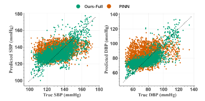
Fig. 4 visually compares the beat-to-beat SBP and DBP estimations using the Ours-Full model and PINN model. The results clearly demonstrate the effectiveness of the proposed model. Under identical training constraints, it is evident that the Ours-Full model outperforms the PINN model in capturing the personalized characteristics of subjects, yielding higher correlations and lower absolute errors. Ours-Full model consistently outperforms the PINN model across all three signal types (bioimpedance, mmWave, and PPG). Cardiovascular time series data typically involve intricate temporal patterns, where multiple variations (e.g., rising, falling, fluctuation) mix and overlap, making temporal variation modeling extremely challenging. Compared to the vanilla PINN, our PITN model is better equipped to capture such temporal information, resulting in a closer fit to the actual blood pressure values.
However, there are still a few failure cases, likely due to the limited number and inconsistent sampling observed points for certain subjects in the Blumio dataset. Additional training data could potentially improve the model’s accuracy in BP estimation. Generally, the BioZ datasets (Ring-CPT and Graphene-HGCPT) contain more samples, leading to better model performance compared to the Blumio dataset.
As a proof-of-concept, Fig. 5 presents Pearson’s correlation visual analysis, by using subject #5 from the Graphene-HGCPT as an example. We can clearly observe that the prediction points of the Ours-Full model are more closely aligned with the dashed line (where predicted values equal true values), while those of the PINN model are more dispersed. This further demonstrates the effectiveness of our proposed methods in personal modeling and in capturing discriminative variations and cardiovascular dynamics.
V-F Ablation Study
In this subsection, we conduct ablation studies to examine the effectiveness of the proposed temporal block, adversarial training, and contrastive learning, respectively.
| Graphene-HGCPT | Ring-CPT | |||||||||||
|---|---|---|---|---|---|---|---|---|---|---|---|---|
| Method | Corr | RMSE | Corr | RMSE | ||||||||
| Model Name | Temporal block | Adversarial | Contrastive | SBP | DBP | SBP | DBP | SBP | DBP | SBP | DBP | |
| PINN [6] | ✗ | ✗ | ✗ | 0.48 | 0.50 | 12.8 | 11.1 | 0.66 | 0.67 | 8.7 | 6.0 | |
| Ours-Base | ✓ | ✗ | ✗ | +0.12 | +0.06 | -1.4 | -0.8 | +0.08 | +0.02 | -1.7 | -0.5 | |
| Ours w/ adv | ✓ | ✓ | ✗ | +0.13 | +0.05 | -1.7 | -0.9 | +0.09 | +0.03 | -1.9 | -0.8 | |
| Ours-Full | ✓ | ✓ | ✓ | +0.15 | +0.07 | -1.8 | -1.0 | +0.11 | +0.05 | -2.0 | -0.8 | |
V-F1 Temporal Block
As shown in Table IV, with temporal modeling, the Ours-Base model outperforms the vanilla PINN model by a large margin. From the table, we can observe that our proposed temporal blocks have a significant influence on BP prediction, removing them will lead to a significant drop in performance. This demonstrates the vital significance of the proposed temporal block. In terms of Pearson correlation, Ours-Base excels the vanilla PINN by relatively 25% and 12% in SBP and DBP estimation, while in terms of RMSE, Ours-Base outperforms the vanilla PINN by 11% and 3% relatively in SBP and DBP estimation.
V-F2 Adversarial Training
As shown in Table IV, we can see augmenting the framework with adversarial samples (denoted as “Ours w/ adv”) enhances performance compared to the Ours-Base model, which utilizes only clean samples for training. This improvement suggests that minor perturbations in adversarial samples can enhance model performance, especially when training data is insufficient. Although these adversarial samples are designed to introduce perturbations through negative gradients, careful control of the generation steps and perturbations allows them to supplement the training data rather than disrupt it.
It is evident from Fig. 6 that, although the generated adversarial examples exhibit differences in signal characteristics compared to the clean examples, their primary feature components remain closely aligned with the corresponding clean examples. Additionally, we compare various data augmentation methods in the supplementary material to further demonstrate the superiority of our approach.
However, as also shown in Table IV, while adversarial examples improve the framework’s performance on RMSE in two datasets, they may degrade Pearson’s correlation between the estimated and true BP values. To address this, we introduce contrastive learning to better capture BioZ signals with similar BP values, thereby improving correlation.

V-F3 Contrastive Learning
As shown in Table IV, our full model achieves the best correlation between state-of-the-art methods and the Ours-Base model, demonstrating the effectiveness of incorporating contrastive learning to capture BP flow changes over time. As noted in [6], an increase in input BioZ data causes correlation to fluctuate. Thus our proposed contrastive learning approach addresses this issue by introducing an additional loss on bioimpedance signals that have relatively similar BP labels. As anticipated, by aligning bioimpedance signals with similar BP values, our framework can better capture BP dynamics, resulting in improved Pearson’s correlation coefficients. Furthermore, by precisely modeling personal discriminative variations, our full model obtained slightly better performance in RMSE compared to the base model. Overall, it can be observed that, compared to the Ours-Base model, our full model effectively learns cardiovascular dynamics and personal discriminative variations.
VI Conclusion
In this paper, we presented an adversarial contrastive learning-based Physics-Informed Temporal Network for cuffless blood pressure estimation. Specifically, we introduced a temporal block within Physics-informed neural networks to extract intraperodic physiological features for temporal modeling. Additionally, we implemented adversarial training combined with contrastive learning to augment physiological time series data. Extensive experiments conducted on multimodal signals from the graphene-HGCPT, ring-CPT, and Blumio datasets, have demonstrated the superior effectiveness of our framework. In the future, we will apply the proposed framework to other medical applications, such as blood sugar monitoring.
References
- [1] D. Kireev, K. Sel, B. Ibrahim, N. Kumar, A. Akbari, R. Jafari, and D. Akinwande, “Continuous cuffless monitoring of arterial blood pressure via graphene bioimpedance tattoos,” Nature Nanotechnology, vol. 17, no. 8, pp. 864–870, 2022.
- [2] L. Zhao, C. Liang, Y. Huang, G. Zhou, Y. Xiao, N. Ji, Y.-T. Zhang, and N. Zhao, “Emerging sensing and modeling technologies for wearable and cuffless blood pressure monitoring,” npj Digital Medicine, vol. 6, pp. 93–108, 2023.
- [3] E. Gomes, C. Liao, O. Shay, and N. Bikhchandani, “A dataset of synchronized signals from wearable cardiovascular monitoring sensors,” 2021. [Online]. Available: https://dx.doi.org/10.21227/3yte-wz05
- [4] S. González, W.-T. Hsieh, and T. P.-C. Chen, “A benchmark for machine-learning based non-invasive blood pressure estimation using photoplethysmogram,” Scientific Data, vol. 10, no. 1, pp. 149–164, 2023.
- [5] K. Sel, D. Osman, N. Huerta, A. Edgar, R. I. Pettigrew, and R. Jafari, “Continuous cuffless blood pressure monitoring with a wearable ring bioimpedance device,” npj Digital Medicine, vol. 6, no. 1, pp. 59–74, 2023.
- [6] K. Sel, A. Mohammadi, R. I. Pettigrew, and R. Jafari, “Physics-informed neural networks for modeling physiological time series for cuffless blood pressure estimation,” npj Digital Medicine, vol. 6, no. 1, pp. 110–125, 2023.
- [7] B. Ibrahim and R. Jafari, “Cuffless blood pressure monitoring from a wristband with calibration-free algorithms for sensing location based on bio-impedance sensor array and autoencoder,” Scientific Reports, vol. 12, no. 1, pp. 319–333, 2022.
- [8] Y. Cao, H. Chen, F. Li, and Y. Wang, “Crisp-bp: Continuous wrist ppg-based blood pressure measurement,” in Proceedings of the 27th Annual International Conference on Mobile Computing and Networking, 2021.
- [9] Y. Liang, A. Zhou, X. Wen, W. Huang, P. Shi, L. Pu, H. Zhang, and H. Ma, “airbp: Monitor your blood pressure with millimeter-wave in the air,” ACM Transactions on Internet of Things, vol. 4, no. 4, pp. 1–32, 2023.
- [10] L. Zhang, G. Wang, and G. B. Giannakis, “Real-time power system state estimation and forecasting via deep unrolled neural networks,” IEEE Transactions on Signal Processing, vol. 67, no. 15, pp. 4069–4077, 2019.
- [11] M. Raissi, P. Perdikaris, and G. E. Karniadakis, “Physics-informed neural networks: A deep learning framework for solving forward and inverse problems involving nonlinear partial differential equations,” Journal of Computational Physics, vol. 378, pp. 686–707, 2019.
- [12] T. Kapoor, H. Wang, A. Núnez, and R. Dollevoet, “Physics-Informed Neural Networks for Solving Forward and Inverse Problems in Complex Beam Systems,” IEEE Transactions on Neural Networks and Learning Systems, vol. 35, no. 5, pp. 5981–5995, 2024.
- [13] W. Xu, Z. Zhou, T. Li, C. Sun, X. Chen, and R. Yan, “Physics-Constraint Variational Neural Network for Wear State Assessment of External Gear Pump,” IEEE Transactions on Neural Networks and Learning Systems, vol. 35, no. 5, pp. 5996–6006, 2024.
- [14] C. Oszkinat, S. E. Luczak, and I. G. Rosen, “Uncertainty Quantification in Estimating Blood Alcohol Concentration From Transdermal Alcohol Level With Physics-Informed Neural Networks,” IEEE Transactions on Neural Networks and Learning Systems, vol. 34, no. 10, pp. 8094–8101, 2023.
- [15] L. Z. Zhao, X. Ding, and B. A. Prakash, “Pinnsformer: A transformer-based framework for physics-informed neural networks,” in International Conference on Learning Representations, 2024.
- [16] C. Ma, P. Zhang, F. Song, Y. Sun, G. Fan, T. Zhang, Y. Feng, and G. Zhang, “KD-Informer: A Cuff-Less Continuous Blood Pressure Waveform Estimation Approach Based on Single Photoplethysmography,” IEEE Journal of Biomedical and Health Informatics, vol. 27, pp. 2219–2230, 2023.
- [17] J. Zhang, S. Zheng, W. Cao, J. Bian, and J. Li, “Warpformer: A multi-scale modeling approach for irregular clinical time series,” in Proceedings of the 29th ACM SIGKDD Conference on Knowledge Discovery and Data Mining, 2023.
- [18] Z. Yu, J. Wang, W. Luo, R. Tse, and G. Pau, “Mpre: Multi-perspective patient representation extractor for disease prediction,” in IEEE International Conference on Data Mining, 2023.
- [19] T. Chen, P. Wang, Z. Fan, and Z. Wang, “Aug-nerf: Training stronger neural radiance fields with triple-level physically-grounded augmentations,” in Proceedings of the IEEE/CVF Conference on Computer Vision and Pattern Recognition, 2022.
- [20] M. Zhang, N. U. Naresh, and Y. He, “Adversarial data augmentation for task-specific knowledge distillation of pre-trained transformers,” in Proceedings of the AAAI Conference on Artificial Intelligence, 2022.
- [21] X. Liu, F. Zhang, Z. Hou, L. Mian, Z. Wang, J. Zhang, and J. Tang, “Self-supervised learning: Generative or contrastive,” IEEE Transactions on Knowledge and Data Engineering, vol. 35, no. 1, pp. 857–876, 2021.
- [22] K.-H. Yu, A. L. Beam, and I. S. Kohane, “Artificial intelligence in healthcare,” Nature Biomedical Engineering, vol. 2, no. 10, pp. 719–731, 2018.
- [23] D. Kiyasseh, T. Zhu, and D. A. Clifton, “Clocs: Contrastive learning of cardiac signals across space, time, and patients,” in International Conference on Machine Learning, 2021.
- [24] X. Guo, L. Tan, C. Gu, Y. Shu, S. He, and J. Chen, “Magwear: Vital sign monitoring based on biomagnetism sensing,” IEEE Transactions on Mobile Computing, pp. 1–14, 2024.
- [25] A. C. Flint, C. Conell, X. Ren, N. M. Banki, S. L. Chan, V. A. Rao, R. B. Melles, and D. L. Bhatt, “Effect of systolic and diastolic blood pressure on cardiovascular outcomes,” New England Journal of Medicine, vol. 381, no. 3, pp. 243–251, 2019.
- [26] J. Zhang, Y. Wu, Y. Chen, and T. Chen, “Health-radio: Towards contactless myocardial infarction detection using radio signals,” IEEE Transactions on Mobile Computing, vol. 21, no. 2, pp. 585–597, 2022.
- [27] M. Qi, Y. Wang, A. Li, and J. Luo, “Sports video captioning via attentive motion representation and group relationship modeling,” IEEE Transactions on Circuits and Systems for Video Technology, vol. 30, no. 8, pp. 2617–2633, 2019.
- [28] M. Qi, Y. Wang, J. Qin, A. Li, J. Luo, and L. Van Gool, “Stagnet: An attentive semantic rnn for group activity and individual action recognition,” IEEE Transactions on Circuits and Systems for Video Technology, vol. 30, no. 2, pp. 549–565, 2019.
- [29] M. Qi, Y. Wang, A. Li, and J. Luo, “Stc-gan: Spatio-temporally coupled generative adversarial networks for predictive scene parsing,” IEEE Transactions on Image Processing, vol. 29, pp. 5420–5430, 2020.
- [30] M. Qi, J. Qin, Y. Yang, Y. Wang, and J. Luo, “Semantics-aware spatial-temporal binaries for cross-modal video retrieval,” IEEE Transactions on Image Processing, vol. 30, pp. 2989–3004, 2021.
- [31] K. Qin, W. Huang, and T. Zhang, “Deep generative model with domain adversarial training for predicting arterial blood pressure waveform from photoplethysmogram signal,” Biomedical Signal Processing and Control, vol. 70, pp. 102 972–102 988, 2021.
- [32] A. Garg, W. Zhang, J. Samaran, R. Savitha, and C.-S. Foo, “An evaluation of anomaly detection and diagnosis in multivariate time series,” IEEE Transactions on Neural Networks and Learning Systems, vol. 33, no. 6, pp. 2508–2517, 2022.
- [33] W. Qian, Y. Zhao, D. Zhang, B. Chen, K. Zheng, and X. Zhou, “Towards a unified understanding of uncertainty quantification in traffic flow forecasting,” IEEE Transactions on Knowledge and Data Engineering, vol. 36, no. 5, pp. 2239–2256, 2024.
- [34] C. Lv, S. Zhang, Y. Tian, M. Qi, and H. Ma, “Disentangled counterfactual learning for physical audiovisual commonsense reasoning,” Advances in Neural Information Processing Systems, 2024.
- [35] N. F. Ali and M. Atef, “An efficient hybrid lstm-ann joint classification-regression model for ppg based blood pressure monitoring,” Biomedical Signal Processing and Control, vol. 84, pp. 104 782–104 793, 2023.
- [36] D. Barvik, M. Cerny, M. Penhaker, and N. Noury, “Noninvasive continuous blood pressure estimation from pulse transit time: A review of the calibration models,” IEEE Reviews in Biomedical Engineering, vol. 15, pp. 138–151, 2021.
- [37] C. Xie, M. Tan, B. Gong, J. Wang, A. L. Yuille, and Q. V. Le, “Adversarial examples improve image recognition,” in Proceedings of the IEEE/CVF Conference on Computer Vision and Pattern Recognition, 2020.
- [38] A. Ilyas, S. Santurkar, D. Tsipras, L. Engstrom, B. Tran, and A. Madry, “Adversarial examples are not bugs, they are features,” Advances in Neural Information Processing Systems, 2019.
- [39] D. Tsipras, S. Santurkar, L. Engstrom, A. Turner, and A. Madry, “There is no free lunch in adversarial robustness (but there are unexpected benefits),” arXiv preprint arXiv:1805.12152, vol. 2, no. 3, 2018.
- [40] D. Yin, R. Gontijo Lopes, J. Shlens, E. D. Cubuk, and J. Gilmer, “A fourier perspective on model robustness in computer vision,” Advances in Neural Information Processing Systems, 2019.
- [41] M. Ivgi and J. Berant, “Achieving model robustness through discrete adversarial training,” in Conference on Empirical Methods in Natural Language Processing, 2021.
- [42] H. He, Q. Zhang, S. Wang, K. Yi, Z. Niu, and L. Cao, “Learning informative representation for fairness-aware multivariate time-series forecasting: A group-based perspective,” IEEE Transactions on Knowledge and Data Engineering, vol. 36, no. 6, pp. 2504–2516, 2024.
- [43] Y. Li, S. Shi, Z. Guo, and B. Wu, “Adversarial training for physics-informed neural networks,” arXiv preprint arXiv:2310.11789, 2023.
- [44] X. Wu, C.-D. Wang, J.-Q. Lin, W.-D. Xi, and P. S. Yu, “Motif-based contrastive learning for community detection,” IEEE Transactions on Neural Networks and Learning Systems, vol. 35, no. 9, pp. 11 706–11 719, 2024.
- [45] J. Qin, Z. Yang, J. Chen, X. Liang, and L. Lin, “Template-based contrastive distillation pretraining for math word problem solving,” IEEE Transactions on Neural Networks and Learning Systems, vol. 35, no. 9, pp. 12 823–12 835, 2024.
- [46] T. Chen, S. Kornblith, M. Norouzi, and G. Hinton, “A simple framework for contrastive learning of visual representations,” in International Conference on Machine Learning, 2020.
- [47] T. Gao, X. Yao, and D. Chen, “Simcse: Simple contrastive learning of sentence embeddings,” in Conference on Empirical Methods in Natural Language Processing, 2021.
- [48] D. Spathis, I. Perez-Pozuelo, L. Marques-Fernandez, and C. Mascolo, “Breaking away from labels: The promise of self-supervised machine learning in intelligent health,” Patterns, vol. 3, no. 2, 2022.
- [49] K. He, X. Zhang, S. Ren, and J. Sun, “Deep residual learning for image recognition,” in Proceedings of the IEEE/CVF Conference on Computer Vision and Pattern Recognition, 2016.
- [50] T. Zhou, Z. Ma, Q. Wen, X. Wang, L. Sun, and R. Jin, “Fedformer: Frequency enhanced decomposed transformer for long-term series forecasting,” in International Conference on Machine Learning, 2022.
- [51] C. Szegedy, W. Liu, Y. Jia, P. Sermanet, S. Reed, D. Anguelov, D. Erhan, V. Vanhoucke, and A. Rabinovich, “Going deeper with convolutions,” in Proceedings of the IEEE/CVF Conference on Computer Vision and Pattern Recognition, 2015.
- [52] A. Madry, A. Makelov, L. Schmidt, D. Tsipras, and A. Vladu, “Towards deep learning models resistant to adversarial attacks,” in International Conference on Learning Representations, 2018.
- [53] B. U. Demirel and C. Holz, “Finding Order in Chaos: A Novel Data Augmentation Method for Time Series in Contrastive Learning,” Advances in Neural Information Processing Systems, 2023.
- [54] P. Khosla, P. Teterwak, C. Wang, A. Sarna, Y. Tian, P. Isola, A. Maschinot, C. Liu, and D. Krishnan, “Supervised contrastive learning,” Advances in Neural Information Processing Systems, 2020.
- [55] F. Schrumpf, P. Frenzel, C. Aust, G. Osterhoff, and M. Fuchs, “Assessment of non-invasive blood pressure prediction from ppg and rppg signals using deep learning,” Sensors, vol. 21, no. 18, p. 6022, 2021.
- [56] Y. Liu, T. Hu, H. Zhang, H. Wu, S. Wang, L. Ma, and M. Long, “itransformer: inverted transformers are effective for time series forecasting,” in International Conference on Learning Representations, 2024.
- [57] H. Wu, T. Hu, Y. Liu, H. Zhou, J. Wang, and M. Long, “Timesnet: Temporal 2d-variation modeling for general time series analysis,” in International Conference on Learning Representations, 2023.
- [58] G. S. Stergiou, B. Alpert, S. Mieke, R. Asmar, N. Atkins, S. Eckert, G. Frick, B. Friedman, T. Graßl, T. Ichikawa et al., “A universal standard for the validation of blood pressure measuring devices: Association for the advancement of medical instrumentation/european society of hypertension/international organization for standardization (aami/esh/iso) collaboration statement,” Hypertension, vol. 71, no. 3, pp. 368–374, 2018.
- [59] G. D. Ruxton, “The unequal variance t-test is an underused alternative to student’s t-test and the mann–whitney u test,” Behavioral Ecology, vol. 17, no. 4, pp. 688–690, 2006.