^†^†institutetext: School of Physics, Beihang University, Beijing 100191, China

Pinning down the primordial black hole formation mechanism with gamma-rays and gravitational waves

Abstract

Primordial black holes (PBHs) are predicted in many models via different formation mechanisms. Identifying the origin of PBHs is of the same importance as probing their existence. We propose to probe the asteroid-mass PBHs [ $\mathcal{O}(10^{17})~{}{\rm g}\lesssim M\lesssim\mathcal{O}(10^{22})~{}{\rm g}$ ] with gamma-rays from Hawking radiation and the stochastic gravitational waves (GWs) from the early Universe. We consider four concrete formation mechanisms, including collapse from primordial curvature perturbations, first-order phase transitions, or cosmic strings, and derive the extended PBH mass functions of each mechanism for phenomenological study. The results demonstrate that by combining gamma-rays and GW signals we can probe PBHs up to $\mathcal{O}(10^{19})~{}{\rm g}$ and identify their physical origins.

1 Introduction

Many models predict the formation of black holes in the early Universe, soon after the Big Bang. Those primordial black holes (PBHs), in contrast to “astrophysical” black holes that are formed from stellar collapses, exist long before the formation of galaxies and stars zel1967hypothesis ; hawking1971gravitationally . Therefore, the mass of PBHs is not necessarily related to the stellar mass and can be in a vast range, depending on the formation mechanism. Different mass ranges receive experimental probes from different astrophysical or cosmological observations. Due to the Hawking radiation Hawking:1974rv , PBHs with mass $M\lesssim 5\times 10^{14}$ g would have evaporated before today and could leave their imprints in the Big Bang Nucleosynthesis (BBN) Carr:2009jm , Cosmic Microwave Background (CMB) Acharya:2020jbv ; Chluba:2020oip , extragalactic gamma-rays Carr:2009jm , or gravitational waves Papanikolaou:2020qtd ; Papanikolaou:2022chm ; Papanikolaou:2021uhe ; Papanikolaou:2022hkg . Heavier PBHs can survive till today and be probed by gamma-rays (for $M\lesssim 10^{19}$ g), gravitational microlensing (for $M\gtrsim 10^{21}$ g), accretion (for $10^{34}~{}{\rm g}\lesssim M\lesssim 10^{41}~{}{\rm g}$ ), etc. See Refs. Carr:2020gox ; Carr:2020xqk ; Green:2020jor for reviews on current constraints on PBHs.

Depending on their masses, PBHs have very rich cosmological implications. Light PBHs can Hawking evaporate into dark matter (DM) Bell:1998jk ; Khlopov:2004tn ; Allahverdi:2017sks ; Lennon:2017tqq ; Gondolo:2020uqv ; Masina:2020xhk ; Bernal:2021yyb ; Cheek:2021odj ; Cheek:2021cfe ; Sandick:2021gew ; Cheek:2022mmy , dark radiation Hooper:2019gtx ; Masina:2021zpu ; Arbey:2021ysg ; Cheek:2022dbx or generate the baryon asymmetry of the Universe Toussaint:1978br ; Turner:1979bt ; Grillo:1980rt ; Baumann:2007yr ; Fujita:2014hha ; Hook:2014mla ; Hamada:2016jnq ; Morrison:2018xla ; Bernal:2022pue ; Hooper:2020otu ; Perez-Gonzalez:2020vnz ; Datta:2020bht ; JyotiDas:2021shi ; Gehrman:2022imk . PBHs with tens to hundreds of the solar mass ( $M_{\odot}$ ) might explain the merger signals observed by the LIGO/Virgo collaborations LIGOScientific:2016aoc ; LIGOScientific:2016sjg ; LIGOScientific:2017bnn ; Clesse:2016vqa ; Bird:2016dcv ; Sasaki:2016jop . Even heavier PBHs, with $M\gtrsim\mathcal{O}(10^{3}-10^{5})M_{\odot}$ , could seed the superheavy black holes Bean:2002kx ; Khlopov:2004sc ; Duechting:2004dk ; Kawasaki:2012kn ; Clesse:2015wea ; DeLuca:2022bjs . Especially, PBHs with $\mathcal{O}(10^{17})~{}{\rm g}\lesssim M\lesssim\mathcal{O}(10^{22})~{}{\rm g}$ , known as the “asteroid-mass range”, can still explain all the DM abundance Carr:2020xqk . It is well known that asteroid-mass PBHs can be probed by Hawking radiation.¹¹1There are also other approaches to probe this mass range, such as gamma-ray burst lensing Jung:2019fcs . Indeed, the existing astronomical observations on gamma-rays Laha:2020ivk ; Coogan:2020tuf ; Laha:2019ssq ; DeRocco:2019fjq , $e^{\pm}$ and neutrinos Boudaud:2018hqb ; Dasgupta:2019cae have put stringent bounds on $f_{\rm pbh}$ , i.e. the fraction of DM contributed by PBHs. For a monochromatic PBH mass function, the upper bound on $f_{\rm pbh}$ varies approximately from $10^{-8}$ to 1 for $M$ ranging from $10^{15}$ g to $10^{17}$ g, with an $M^{4}$ scaling Carr:2020gox ; Carr:2020xqk ; Green:2020jor . Future gamma-ray detectors are able to probe PBH DM candidate up to $\mathcal{O}(10^{19})~{}{\rm g}$ Coogan:2020tuf ; Ray:2021mxu ; Ghosh:2021gfa .

In this article, we propose to probe asteroid-mass PBHs with near-future gamma-ray detectors and gravitational wave (GW) detectors. Instead of phenomenologically assuming a monochromatic PBH mass function, we consider concrete physical mechanisms of PBH formation, which yield extended mass functions and hence predict more realistic gamma-ray signal spectra. The four mechanisms under consideration are

1.

Collapse of overdense regions originating from curvature perturbations generated during inflation Carr:1974nx ; Carr:1975qj ;
2.

Direct collapse of false vacuum remnants during a cosmic first-order phase transition (FOPT) Baker:2021nyl ; Baker:2021sno ;
3.

Subsequent collapse of non-topological solitons which are formed in a FOPT Kawana:2021tde ;
4.

Collapse of cosmic strings Hawking:1987bn .

Remarkably, all those mechanisms have stochastic GW companions. This provides us the opportunity to probe the origin of PBHs via multi-messenger astronomy. An analysis of correlating gamma-ray and GWs from the curvature perturbation PBH mechanism is performed in Ref. Agashe:2022jgk , showing the possibility of testing the above formation mechanism 1. In current article, we for the first time discuss the comparison and identification of signals from different PBH mechanisms via multi-messenger astronomy.

This work discusses the main features of gamma-ray and GW signals from concrete formation mechanisms, demonstrating that they are qualitatively distinguishable. For a quantitative study, we consider the MeV gamma-ray detectors e-ASTROGAM e-ASTROGAM:2016bph and AMEGO-X Fleischhack:2021mhc , which are planed for launch at the end of the 2020s; and a few GW detectors, which are already under operation or proposed to start data-taking in the 2030s, including the pulsar timing arrays (PTAs) NANOGrav McLaughlin:2013ira ; NANOGRAV:2018hou ; Aggarwal:2018mgp ; Brazier:2019mmu , PPTA Manchester:2012za ; Shannon:2015ect , EPTA Kramer:2013kea ; Lentati:2015qwp ; Babak:2015lua , IPTA Hobbs:2009yy ; Manchester:2013ndt ; Verbiest:2016vem ; Hazboun:2018wpv and SKA Carilli:2004nx ; Janssen:2014dka ; Weltman:2018zrl , the space-based laser interferometers LISA LISA:2017pwj , TianQin TianQin:2015yph ; Hu:2017yoc ; TianQin:2020hid , Taiji Hu:2017mde ; Ruan:2018tsw , BBO Crowder:2005nr and DECIGO Kawamura:2011zz , and the ground-based interferometers LIGO LIGOScientific:2014qfs ; LIGOScientific:2019vic , CE Reitze:2019iox and ET Punturo:2010zz ; Hild:2010id ; Sathyaprakash:2012jk . Our research shows that, after combining gamma-ray and GW signals, we can probe the existence of PBHs with mass up to $\mathcal{O}(10^{19})~{}{\rm g}$ , and equally importantly identify their physical origin.

This article is organized as follows. We first introduce the four PBH mechanisms one by one in Section 2 (curvature perturbations), Section 3.2 (direct collapse during a FOPT), Section 3.3 (collapse of non-topological solitons from a FOPT), and Section 4 (cosmic strings), and discuss the corresponding gamma-ray and GW signals, as well as their correlations. Then in Section 5 we summarize our results with a combined discussion of different mechanisms, pointing out how to distinguish them in future experiments. The conclusion is also given.

2 PBHs from curvature perturbations

Large scalar perturbation generated by inflationary theories can source PBH formation Carr:1975qj ; Ivanov:1994pa ; Garcia-Bellido:1996mdl ; Silk:1986vc ; Kawasaki:1997ju ; Yokoyama:1995ex ; Choudhury:2013woa ; Di:2017ndc ; Pi:2017gih ; Hertzberg:2017dkh ; Ballesteros:2017fsr ; Cai:2018dig ; Dalianis:2018frf ; Ozsoy:2018flq ; Cicoli:2018asa ; ShamsEsHaghi:2022azq ; Choudhury:2023vuj . While the Universe is confirmed to be nearly homogeneous at large scales by measurements of Lyman- $\alpha$ forest Bird:2010mp , CMB anisotropy Planck:2018jri and CMB distortion Mather:1993ij ; Fixsen:1996nj , small scale fluctuations are still less constrained. For example, the matter power spectrum of curvature perturbations $P_{\zeta}$ could be enhanced during inflation when the inflaton field undergoes a temporary ultra slow-roll phase Martin:2012pe ; Kinney:2005vj ; Germani:2017bcs ; Dimopoulos:2017ged ; Riotto:2023hoz ; Kawai:2021edk ; Kawai:2021bye ; Kawai:2022emp ; Wang:2022nml . The fluctuations, after being produced, become super-horizon modes and stay frozen until they enter the causal horizon as overdense regions much after the end of the inflation epoch. After horizon reentry, PBHs are formed from the direct collapse of dense horizon patches whose distribution are determined by $P_{\zeta}(k)$ , where $k$ is the comoving wave number. Gravitational collapse happens when density contrast $\delta$ in the horizon becomes larger than the threshold value $\delta_{c}$ . We adopt the Press-Schechter (PS) formalism Press:1973iz for the calculation of PBH abundance with the assumption that density contrasts in the early Universe follow a Gaussian distribution

\displaystyle p(\delta)=\frac{1}{\sqrt{2\pi\sigma^{2}_{0}}}\,e^{-\frac{\delta^{2}}{2\sigma^{2}_{0}}}.

(1)

Here the mean value of $\delta$ is zero, because the Universe is nearly homogeneous and the overdense and underdense regions appear with equal probabilities. The variance is given by

\sigma_{0}^{2}(R)=\displaystyle{\int_{0}^{\infty}}\frac{{\rm d}k^{\prime}}{k^{\prime}}\frac{16}{81}(k^{\prime}R)^{4}W^{2}(k^{\prime},R)P_{\zeta}(k^{\prime}),

(2)

where $R=1/(Ha)$ is the comoving Hubble radius, with $H$ the Hubble rate and $a$ the scale factor. A window function $W(k^{\prime},R)$ is used to smooth the density contrast, which we take to be Gaussian in this study

W(k^{\prime},R)=\exp\left(-\frac{(k^{\prime}R)^{2}}{4}\right).

(3)

Since a comoving Hubble radius $R$ corresponds to a reentry wave number $k\equiv R^{-1}$ , $\sigma_{0}^{2}$ can also be treated as a function of $k$ via Eq. (2).

Horizon patches with $\delta>\delta_{c}$ collapse to PBHs with mass Choptuik:1992jv ; Niemeyer:1997mt ; Niemeyer:1999ak

M=M_{H}K(\delta-\delta_{c})^{\gamma_{r}},

(4)

where $M_{H}$ is the horizon mass as a function of $R$ , and we use $\delta_{c}=0.55$ , $K=10$ and $\gamma_{r}=0.36$ Musco:2020jjb ; Escriva:2021aeh . The energy density ratio of PBH to radiation, $\beta_{\rm pbh}$ , is

\frac{\partial^{2}\beta_{\rm pbh}}{\partial\delta\partial\log R}=\frac{2M}{M_{H}}p(\delta),\quad\delta\geqslant\delta_{c},

(5)

at the moment of PBH formation. To get the PBH distribution today, we take into account the cosmic expansion, reheating from the decoupling of Standard Model (SM) particle species and the PBH mass loss via Hawking evaporation,

\frac{\text{d}f_{\rm pbh}}{\text{d}M}=\frac{\Omega_{m}h^{2}}{\Omega_{\rm DM}h^{2}}\left(\frac{M}{M^{\prime}}\right)^{3}\frac{\text{d}\beta_{\rm pbh}^{\rm eq}}{\text{d}M}\Big{|}_{M\to M^{\prime}},

(6)

where $M^{\prime}=(M^{3}+3f_{0}t_{0}M_{\rm Pl}^{4})^{1/3}$ , and

\frac{\text{d}\beta_{\rm pbh}^{\rm eq}}{\text{d}M}=\int_{0}^{\rm R_{\rm eq}}\frac{\text{d}R}{R}\frac{R_{\rm eq}}{R}\left(2\frac{g_{*}(T_{i})}{g_{*}(T_{\rm eq})}\frac{g_{*s}^{4/3}(T_{\rm eq})}{g_{*s}^{4/3}(T_{i})}\right)^{1/2}\frac{\partial^{2}\beta_{\rm pbh}}{\partial\delta\partial\log R}\frac{\text{d}\delta}{\text{d}M},

(7)

is the ratio of PBH energy density to radiation at matter-radiation equality Agashe:2022jgk . $g_{*}$ and $g_{*s}$ are the numbers of relativistic degrees of freedom for energy and entropy, respectively, and the variables labeled with subscript “eq” and “ $i$ ” are given at matter-radiation equality and PBH formation time, respectively. The abundances of matter and cold DM are $\Omega_{m}h^{2}\approx 0.142$ and $\Omega_{\rm DM}h^{2}\approx 0.120$ , respectively ParticleDataGroup:2020ssz . The PBH evaporation parameter is $f_{0}=1.895\times 10^{-3}$ Hooper:2019gtx and the age of the present Universe is $t_{0}=4.6\times 10^{17}~{}{\rm s}$ .

Given a curvature perturbation $P_{\zeta}(k)$ , one can derive $\text{d}f_{\rm pbh}/\text{d}M$ via the above procedure. If $P_{\zeta}(k)$ is enhanced at some specific $k$ -mode $k_{p}$ , when the enhanced mode reenters the horizon, the variance $\sigma_{0}(R)$ is also enhanced and hence large density contrast could exist. This generates a peak in the PBH mass function. In this article, we parametrize the curvature perturbation using a log-normal function

P_{\zeta}(k)=\frac{A}{\sqrt{2\pi\sigma^{2}}}\,\exp\left(\frac{\log^{2}\left(k/k_{p}\right)}{2\sigma^{2}}\right).

(8)

By this setup, given a set of $(A,k_{p},\sigma)$ , one can derive the mass function $\text{d}f_{\rm pbh}/\text{d}M$ . The non-linear relation between the density contrast and curvature perturbations requires $\sim 2$ larger $P_{\zeta}$ , and this extra factor is included in our calculation Young:2019yug . Once $\text{d}f_{\rm pbh}/\text{d}M$ is available, the gamma-ray spectrum can be evaluated with the method described in Appendix A.

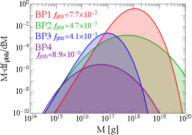
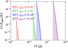
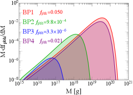
The input parameters $(A,k_{p},\sigma)$ affect the PBH mass function in a very clear way: $A$ controls $f_{\rm pbh}$ , $k_{p}$ determines the peak position of $M$ , while $\sigma$ dominates the width of the mass peak, as shown in the parameter scan of Ref. Agashe:2022jgk . For four benchmark points (BPs)

\{A,~{}k_{p},~{}\sigma\}=\begin{cases}~{}\{10^{-1.26},~{}3\times 10^{14}~{}{\rm Mpc}^{-1},~{}2\},&{\rm BP1};\\ ~{}\{10^{-1.03},~{}3\times 10^{14}~{}{\rm Mpc}^{-1},~{}4\},&{\rm BP2};\\ ~{}\{10^{-1.33},~{}10^{15}~{}{\rm Mpc}^{-1},~{}2\},&{\rm BP3};\\ ~{}\{10^{-1.10},~{}10^{15}~{}{\rm Mpc}^{-1},~{}4\},&{\rm BP4},\\ \end{cases}

(9)

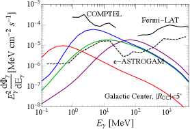
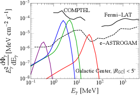
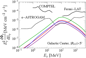
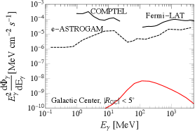
we plot the PBH mass functions in the left panel of Fig. 1. The BPs are selected based on the consideration that they should produce asteroid-mass PBHs, and should not be ruled out by current gamma-ray observations, and have $f_{\rm pbh}\leqslant 1$ . This leads to BPs with $k_{p}\sim 10^{15}~{}{\rm Mpc}^{-1}$ with various $A$ and $\sigma$ values. We can see the mass peaks match the estimation in Eq. (4), and a larger $\sigma$ of the power spectrum yields a broader PBH mass distribution. The corresponding gamma-ray spectra are plotted in the right panel of Fig. 1, where the signals are from the galactic center with an angle extent $|R_{\rm GC}|\leqslant 5^{\circ}$ . In the same figure, we also add the current constraints from gamma-ray observations Fermi-LAT Fermi-LAT:2017opo , COMPTEL 1998PhDT………3K and the projections from e-ASTROGAM e-ASTROGAM:2016bph , all rescaled to the region of interest (ROI) of our study. In particular, we take the COMPTEL constraint from Essig:2013goa . The projected reach of e-ASTROGAM is derived by rescaling the expected background numbers provided by Ref. e-ASTROGAM:2016bph to our ROI and requiring a $2\sigma$ deviation contributed by the signals in each bin. We expect the AMEGO-X Fleischhack:2021mhc detector has a similar sensitivity.

Refer to caption — Figure 1: The current mass distributions (left) and corresponding gamma-ray spectra (right) of the PBHs from curvature perturbations. The description of the BPs can be found in Eq. (9).

Curvature perturbations can source stochastic GWs via tensor mode produced at the second-order. The effect of induced GWs from scalar perturbations is studied in Refs. 1967PThPh..37..831T ; Mollerach:2003nq ; Ananda:2006af ; Baumann:2007zm ; Acquaviva:2002ud ; Yuan:2021qgz ; Domenech:2021ztg ; Pi:2020otn ; Kohri:2018awv ; Espinosa:2018eve ; Braglia:2020eai ; Inomata:2019ivs ; Inomata:2016rbd ; Inomata:2018epa ; Kozaczuk:2021wcl ; Agashe:2022jgk . Here we follow Refs. Kozaczuk:2021wcl ; Agashe:2022jgk for the calculation in our analysis. The GW spectrum is defined as the GW energy density fraction as a function of the frequency,

\Omega_{\rm GW}(f)=0.83\left(\frac{g_{*s}(T_{c})}{10.75}\right)^{-\frac{1}{3}}\Omega_{r,0}\Omega_{\rm GW}(\eta_{c},k),

(10)

with $\Omega_{r,0}=8.5\times 10^{-5}$ being the current radiation abundance, respectively; and $\eta_{c}$ and $T_{c}$ are the reentry conformal time and temperature determined by $k$ , respectively. The $k$ -mode is related to GW frequency via

f_{\rm GW}=1.546~{}{\rm Hz}\times\left(\frac{k}{10^{15}~{}{\rm Mpc}^{-1}}\right),

(11)

which indicates the peak frequency of GWs is determined by the horizon reentry of enhanced $k$ -mode of $P_{\zeta}(k)$ .

The full expression of GW energy fraction at a given $k$ at conformal time $\eta$ is

\Omega_{\rm GW}(\eta,k)=\frac{1}{24}\left(\frac{k}{a(\eta)H(\eta)}\right)^{2}P_{h}(\eta,k),

(12)

with the power spectrum of the GW being

P_{h}(\eta,k)\simeq 2\int^{\infty}_{0}\text{d}t\int^{1}_{-1}\text{d}s\left(\frac{t(t+2)(s^{2}-1)}{(t+s+1)(t-s+1)}\right)^{2}I^{2}(s,t,k\eta)P_{\zeta}(uk)P_{\zeta}(vk).

(13)

The $I^{2}$ function can be calculated when the GWs are deeply in the sub-horizon limit. In that limit, the growth of GW amplitude is terminated by the decay of the enhanced $k$ -mode once it is much smaller than the horizon size. In this limit, we can take

\begin{split}I^{2}(s,t,k\eta)=&~{}\frac{288(s^{2}+t(t+2)-5)^{2}}{k^{2}\eta^{2}(t+s+1)^{6}(t-s+1)^{6}}\left[\frac{\pi^{2}}{4}(s^{2}+t(t+2)-5)^{2}\Theta(t-(\sqrt{3}-1))\right.\\ &~{}\left.+\left((t+s+1)(s-t-1)+\frac{s^{2}+t(t+2)-5}{2}\log\left|\frac{t(t+2)-2}{3-s^{2}}\right|\right)^{2}\right],\end{split}

(14)

where $\Theta$ is the Heaviside function.

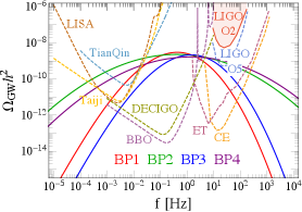
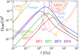
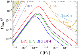
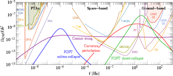
Since the PBH mass is proportional to $k^{-2}$ , the curvature perturbation responsible for the generation of heavy (light) PBHs lies in the lower (higher) frequency regions. For PBH mass in the asteroid-mass window, the target GW signals have $\sim\text{Hz}$ frequency, as implied by Eq. (4) and Eq. (11). The abundance of GWs $\Omega_{\rm GW}$ is quadratic in the amplitude of the power spectrum $P_{\zeta}(k)$ . As the amplitude is required to be larger than $\sim 10^{-2}$ for sufficient PBH formation, the GWs are estimated to make up $10^{-4}$ of the energy density of the Universe at the horizon-reentry time, and then redshift to $10^{-9}$ in the current Universe. This is within the sensitive region of a few ground-based and proposed space-based GW detectors, as illustrated in Fig. 2. The signals are best probed by the future BBO Crowder:2005nr and DECIGO Kawamura:2011zz detectors, but the near-future LISA LISA:2017pwj , TianQin TianQin:2015yph ; Hu:2017yoc ; TianQin:2020hid , Taiji Hu:2017mde ; Ruan:2018tsw , CE Reitze:2019iox and ET Punturo:2010zz ; Hild:2010id ; Sathyaprakash:2012jk , or even the operating LIGO LIGOScientific:2014qfs ; LIGOScientific:2019vic , also have considerable sensitivities to probe them. Combining the gamma-ray and GW signals, we can efficiently probe the curvature perturbation-induced PBH scenario, and this has been pointed out by Ref. Agashe:2022jgk .

3 PBHs from a FOPT

3.1 The general mechanism

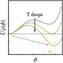
Suppose the Universe is filled up with a scalar field $\phi$ , whose effective potential $U_{T}(\phi)$ evolves with the temperature $T$ Quiros:1999jp . The vacuum is initially at the field space origin $\phi=0$ , where the Universe stays at. As $T$ drops, the potential develops another deeper local minimum, or say, “the true vacuum”, away from the origin. If the two vacua are separated by a potential barrier, the Universe cannot smoothly shift to the true vacuum, but can only decay to it through quantum tunneling Linde:1981zj , as illustrated in the left panel of Fig. 3. This is known as a FOPT, which happens in spacetime via vacuum bubble nucleation and expansion. Inside the bubble is the new true vacuum with $\phi\neq 0$ , while outside the bubble is the old false vacuum with $\phi=0$ . The FOPT completes when the bubbles eventually fulfill the entire space, converting the whole Universe to the true vacuum.

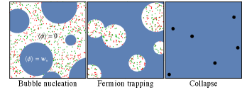
If there is a fermion species $\chi$ that couples to the scalar field $\phi$ via $\mathcal{L}\supset\bar{\chi}i\not{\partial}\chi-y_{\chi}\phi\bar{\chi}\chi$ , then during the FOPT $\chi$ would be massless outside the bubble, but gain a mass $m_{\chi}=y_{\chi}w_{*}$ inside the bubble, where $w_{*}$ is the vacuum expectation value (VEV) of $\phi$ at the true vacuum at FOPT temperature $T_{*}$ . If the mass gap $m_{\chi}\gg T_{*}$ , then most of the fermions are not able to penetrate into the true vacuum because the kinetic energy is $\mathcal{O}(T_{*})$ Baker:2019ndr ; Chway:2019kft ; Chao:2020adk ; Deng:2020dnf . For example, $m_{\chi}=12\,T_{*}$ yields a trapping fraction of 98% when the bubble velocity is $v_{w}=0.6$ Kawana:2021tde ; Hong:2020est . As a result, the fermions are reflected by the bubble walls and hence get trapped in the false vacuum. One can naturally expect that, as the FOPT proceeds, the false vacuum remnants shrink to smaller and smaller sizes, and then the trapped fermions are squeezed, which means the energy density increases rapidly. Those remnants might eventually collapse into PBHs, as sketched in the right panel of Fig. 3.

However, for the false vacuum remnants to be sufficiently dense to collapse into PBHs, we have to address an important issue: how to prevent the trapped fermions from disappearing through $\chi\bar{\chi}\to\phi,~{}\phi\phi$ , etc, and eventually to the SM particles in the thermal bath? Such annihilations are inevitably enhanced when the remnants shrink, reducing the fermion number density greatly Arakawa:2021wgz ; Asadi:2021yml and consequently destroying any possibility of collapse into PBHs. To have PBHs formed, there are two typical scenarios:

I.

Suppress the annihilation rate by a relatively small Yukawa coupling $y_{\chi}$ Baker:2021nyl ; Baker:2021sno . In this case, the false vacuum remnants directly collapse into PBHs.
II.

Generate a $\chi$ - $\bar{\chi}$ number density asymmetry such that $\chi$ ’s survive the annihilation Kawana:2021tde . In this case, the remnants first shrink to non-topological solitons called “Fermi-balls” Hong:2020est , which could collapse into PBHs due to the internal Yukawa interaction.

We will discuss them one by one in the following subsections. In those scenarios, the distribution of false vacuum remnants is crucial in deriving the PBH mass function. While the numerical study of such a distribution is still lacking, we adopt the analytical technique developed in Ref. Lu:2022paj as a first trial.

3.2 Scenario I: the direct collapse of false vacuum remnants

This scenario is first proposed by Refs. Baker:2021nyl ; Baker:2021sno , which demonstrate that by adopting a small Yukawa coupling

y_{\chi}\lesssim 10^{-4}\left(\frac{T_{*}}{10^{6}~{}{\rm GeV}}\right)^{1/2},

(15)

the annihilation processes $\chi\bar{\chi}\to\phi,~{}\phi\phi$ are suppressed. Note that the trapping condition $m_{\chi}=y_{\chi}w_{*}\gg T_{*}$ requires $w_{*}\gg T_{*}$ when $y_{\chi}$ is small. Once Eq. (15) holds, the energy density of the trapped fermions is approximately

\rho_{\chi}(t)\approx\rho_{\chi}^{\rm eq}\left(\frac{R_{r}^{0}}{R_{r}(t)}\right)^{4},

(16)

where $R_{r}(t)$ is the size of the false vacuum remnant at time $t$ , $R_{r}^{0}\equiv R_{r}(t=t_{*})$ is the initial size with $t_{*}$ being the cosmic time of FOPT, $\rho_{\chi}^{\rm eq}=(7/8)(\pi^{2}g_{\chi}/30)T_{*}^{4}$ is the initial fermion energy density of the remnant (which is just the equilibrium value right before the FOPT), $g_{\chi}=4$ counts the number of the degrees of freedom including both $\chi$ and $\bar{\chi}$ . Eq. (16) includes the number density enhancement $\propto\left(R_{r}^{0}/R_{r}(t)\right)^{3}$ and the energy gain of the fermions from reflections of the bubble wall $\propto R_{r}^{0}/R_{r}(t)$ during the shrinking of $R_{r}(t)$ . The scaling in Eq. (16) is confirmed by the numerical simulations Baker:2021nyl ; Baker:2021sno and the analytical calculations Kawana:2022lba .

As $R_{r}(t)$ decreases, $\rho_{\chi}(t)$ increases and so does the Schwarzschild radius of the remnant,

R_{s}(t)=\frac{2}{M_{\rm Pl}^{2}}\frac{4\pi}{3}R_{r}^{3}(t)\rho_{\chi}(t),

(17)

with $M_{\rm Pl}=1.22\times 10^{19}$ GeV the Planck scale. When $R_{r}(t)<R_{s}(t)$ , the remnant collapses into a black hole. Denote the collapse time as $t_{\rm col}$ , the collapse condition is then

\frac{R_{r}(t_{\rm col})}{R_{r}^{0}}=\sqrt{\frac{7}{8}\frac{g_{\chi}}{g_{*}}}\frac{R_{r}^{0}}{H_{*}^{-1}},

(18)

with $H_{*}^{-1}$ being the Hubble radius at FOPT. Note that the collapse condition is determined by the overdense region of the $\chi/\bar{\chi}$ fermions only.

Eq. (18) implies that, at the moment of PBH formation, the ratio of the remnant size $R_{r}(t_{\rm col})$ to the initial size $R_{r}^{0}$ is proportional to the ratio of $R_{r}^{0}$ to the Hubble radius $H_{*}^{-1}$ . As mentioned, the premise of this scenario is the suppressed $\chi\bar{\chi}$ annihilation, such that we have Eq. (16) and hence Eq. (18); however, the annihilation is extremely difficult to suppress while $R_{r}(t_{\rm col})/R_{r}^{0}$ is too small. Therefore, we can infer that, in this direct collapse scenario, the PBH formation prefers an initial condition with large $R_{r}^{0}/H_{*}^{-1}$ . Indeed, the simulations in Refs. Baker:2021nyl ; Baker:2021sno show successful examples of PBH formation for $R_{r}^{0}=1.5H_{*}^{-1}$ and $2H_{*}^{-1}$ . The resultant PBH mass from the collapse is estimated by the total energy contained in the false vacuum remnant,

M\approx\frac{4\pi}{3}R_{r}^{3}(t_{\rm col})\left(\frac{3M_{\rm Pl}^{2}}{8\pi}H_{*}^{2}\right)=\left(\frac{7g_{\chi}}{8g_{*}}\right)^{3/2}\frac{M_{\rm Pl}^{2}}{2H_{*}}\left(\frac{R_{r}^{0}}{H_{*}^{-1}}\right)^{6},

(19)

and we assume the PBH formation is possible only for $R_{r}^{0}>H_{*}^{-1}$ for simplicity.

According to Eq. (19), to get the mass distribution of $M$ , we should first derive the distribution of the false vacuum remnant size $R_{r}^{0}$ during a FOPT. This can be done using the method proposed by Ref. Lu:2022paj ,

\frac{\text{d}n_{\rm fv}}{\text{d}R_{r}^{0}}\approx\frac{I_{*}^{4}\beta^{4}}{192v_{w}^{3}}e^{(4\beta R_{r}^{0}/v_{w})-I_{*}e^{\beta R_{r}^{0}/v_{w}}}\left(1-e^{-I_{*}e^{\beta R_{r}^{0}/v_{w}}}\right)~{},

(20)

where $n_{\rm fv}$ is the number density of the remnants during the FOPT, $I_{\ast}=-\ln(0.29)=1.238$ , and $\beta$ is the reciprocal of the FOPT duration. Each remnant with radius $R_{r}^{0}$ larger than $H_{*}^{-1}$ collapses into one individual PBH, thus the number density distribution of PBHs at formation is

\frac{\text{d}n_{\rm pbh}^{*}}{\text{d}M}=\frac{\text{d}n_{\rm fv}}{\text{d}R_{r}^{0}}\Big{|}_{R_{r}^{0}>H_{*}^{-1}}\left(\frac{\text{d}M}{\text{d}R_{r}^{0}}\right)^{-1},

(21)

and current PBH distribution should be

\frac{\text{d}f_{\rm pbh}}{\text{d}M}=\left(\frac{M}{M^{\prime}}\right)^{3}\frac{1}{\Omega_{\rm DM}}\left(\frac{8\pi}{3M_{\rm Pl}^{2}H_{0}^{2}}\right)\frac{s_{0}}{s_{*}}\left(M\frac{\text{d}n_{\rm pbh}^{*}}{\text{d}M}\right)\Big{|}_{M\to M^{\prime}},

(22)

where $M^{\prime}=(M^{3}+3f_{0}M_{\rm Pl}^{4}t_{0})^{1/3}$ accounts for the mass loss of PBHs after formation, $s_{0}=2891.2~{}{\rm cm}^{-3}$ is the current entropy density, and $H_{0}=67.4~{}{\rm km/(s\cdot Mpc)}$ is the current Hubble constant ParticleDataGroup:2020ssz .

Eqs. (19)–(22) are used to derive the PBH mass function, and the input parameters are $\{\alpha,~{}\beta/H_{*},~{}T_{*},~{}v_{w}\}$ . As PBHs form only when $R_{r}^{0}>H_{*}^{-1}$ , while $\text{d}n_{\rm fv}/\text{d}R_{r}^{0}$ decreases rapidly with $R_{r}^{0}$ due to the double-exponential suppression factor, we can expect $\text{d}f_{\rm pbh}/\text{d}M$ has a very sharp peak at around

M_{\rm peak}\approx\left(\frac{7g_{\chi}}{8g_{*}}\right)^{3/2}\frac{M_{\rm Pl}^{2}}{2H_{*}}=5.2\times 10^{15}~{}{\rm g}\times\left(\frac{10^{7}~{}{\rm GeV}}{T_{*}}\right)^{2},

(23)

where $g_{*}=g_{\chi}+106.75$ is adopted in the last line. Due to this reason, the gamma-ray signal shape is also very narrow. We perform a parameter scan for $\alpha\in[0,1]$ , $\beta/H_{*}\in[1,10^{3}]$ , $T_{*}\in[10^{-2},10^{8}]~{}{\rm GeV}$ and $v_{w}\in[0.1,0.8]$ , requiring that $M_{\rm peak}$ is in the asteroid-mass range, the gamma-ray signals are allowed by current observations, and $f_{\rm pbh}\leqslant 1$ . The requirement of mass leads to $T_{*}\sim 10^{7}$ GeV, as expected. The gamma-ray signals have narrow shapes at MeV scale, as can be obtained clearly in Fig. 4, where we plot the corresponding mass and gamma-ray spectra in the left and right panels respectively for the four BPs

\{\alpha,~{}\beta/H_{*},~{}T_{*},~{}v_{w}\}=\begin{cases}~{}\{0.0827,~{}2.21,~{}1.65\times 10^{7},~{}0.566\},&{\rm BP1};\\ ~{}\{0.202,~{}1.93,~{}6.22\times 10^{6},~{}0.514\},&{\rm BP2};\\ ~{}\{0.788,~{}2.90,~{}4.58\times 10^{6},~{}0.781\},&{\rm BP3};\\ ~{}\{0.308,~{}1.83,~{}1.68\times 10^{6},~{}0.505\},&{\rm BP4},\\ \end{cases}

(24)

randomly chosen from the scanned results.

FOPT generates stochastic GWs via bubble collisions, sound waves, and turbulences. The resultant GW spectrum, after the cosmological redshift, can be expressed as a function of the FOPT parameters $\{\alpha,\beta/H_{*},T_{*},v_{w}\}$ , namely the ratio of latent heat to the radiation energy density, the inverse ratio of transition duration to the Hubble time, the FOPT temperature and the bubble expansion velocity Caprini:2015zlo ; Caprini:2019egz . For particle trapping scenarios, $v_{w}$ is not extremely close to 1 and hence the dominant contribution to GW spectrum is from the sound waves in the plasma, which yields a peak at Caprini:2015zlo ²²2The amplitude of the GW signal may be suppressed by the finite duration of the sound wave period Ellis:2018mja ; Guo:2020grp . However, in the parameter space of interest, the FOPT duration is typically long that $\beta/H_{*}\lesssim 10$ , and hence the sound wave suppression is not prominent.

\begin{split}f_{\rm peak}\approx&~{}19~{}{\rm Hz}\times\left(\frac{0.1}{v_{w}}\right)\left(\frac{\beta}{H_{*}}\right)\left(\frac{T_{*}}{10^{7}~{}{\rm GeV}}\right)\left(\frac{g_{*}}{100}\right)^{1/6},\\ \Omega_{\rm sw}(f_{\rm peak})h^{2}\approx&~{}2.65\times 10^{-7}\times\left(\frac{\beta}{H_{*}}\right)^{-1}\left(\frac{\kappa_{V}\alpha}{1+\alpha}\right)^{2}\left(\frac{g_{*}}{100}\right)^{-1/3}\left(\frac{v_{w}}{0.1}\right),\end{split}

(25)

where $\kappa_{V}$ is the fraction of released vacuum energy that goes into the plasma kinetic bulk motion Espinosa:2010hh . The corresponding GW signals are within the sensitive region of the ground-based detectors LIGO LIGOScientific:2014qfs ; LIGOScientific:2019vic , CE Reitze:2019iox and ET Punturo:2010zz ; Hild:2010id ; Sathyaprakash:2012jk , or the space-based detectors BBO Crowder:2005nr and DECIGO Kawamura:2011zz . For the four BPs in Eq. (24), we plot the GW spectra in Fig. 5. We have checked that BPs show the representative features (e.g. frequencies, signal strengths) of the scanned parameter points.

Here we provide a short remark for the direct collapse scenario of the FOPT-induced PBHs. Requiring a large false vacuum remnant size $R_{r}^{0}$ , the PBH mass function in this scenario features a sharp peak. As a result, the gamma-ray spectrum also has a very narrow distribution, as illustrated in Fig. 4. The correlated FOPT GW signals are expected to peak at around $\mathcal{O}(10)$ Hz, as shown in Fig. 5.

3.3 Scenario II: collapse of FOPT-induced solitons

This scenario is first proposed by Ref. Kawana:2021tde and then applied in Refs. Marfatia:2021hcp ; Huang:2022him ; Tseng:2022jta ; Kawana:2022lba ; Lu:2022jnp ; Marfatia:2022jiz . A baryogenesis-like mechanism (or say, asymmetric DM Kaplan:2009ag ; Petraki:2013wwa ; Zurek:2013wia ) is introduced to have $n_{\chi}>n_{\bar{\chi}}$ before or during the FOPT, and hence when the fermions are trapped in the false vacuum remnants and forced to annihilate, $\bar{\chi}$ ’s will disappear eventually, but $\chi$ ’s survive. Those residual fermions develop a degeneracy pressure when they are compressed. When that pressure is able to balance the vacuum pressure, a non-topological soliton solution exists, known as the Fermi-ball Hong:2020est . This happens at $\text{d}E_{\rm rem}/\text{d}R_{r}=0$ for the following remnant energy profile

E_{\rm rem}\approx\frac{3\pi}{4}\left(\frac{3}{2\pi}\right)^{2/3}\frac{Q_{\rm FB}^{4/3}}{R_{r}}+\frac{4\pi}{3}\Delta U(T_{*})R_{r}^{3},

(26)

where $R_{r}$ is the remnant radius, $Q_{\rm FB}$ is the charge, i.e. the number of residual fermions trapped in an individual remnant, and $\Delta U(T_{*})$ is the positive vacuum energy difference between the true and false vacua that represents the vacuum pressure that drives the expansion of the bubbles. The Fermi-ball mass and radius are respectively Hong:2020est ³³3Trapping particles to form non-topological soliton is an old idea that receives renewed interest recently. See Refs. Krylov:2013qe ; Huang:2017kzu ; Bai:2022kxq for the Q-balls from a FOPT, and Refs. Witten:1984rs ; Frieman:1990nh ; Zhitnitsky:2002qa ; Oaknin:2003uv ; Lawson:2012zu ; Atreya:2014sca ; Bai:2018vik ; Bai:2018dxf ; Gross:2021qgx for the quark nuggets or dark dwarfs from a QCD-like FOPT.

M_{\rm FB}\approx Q_{\rm FB}\left(12\pi^{2}\Delta U(T_{*})\right)^{1/4},\quad R_{\rm FB}^{3}\approx\frac{3}{16\pi}\frac{M_{\rm FB}}{\Delta U(T_{*})},

(27)

dominated by the charge and vacuum energy difference. Fermi-balls are very dense objects, and they could collapse into PBHs if the internal $\phi$ -mediated Yukawa attractive force between the fermions is too strong Kawana:2021tde . In that case, the daughter PBH inherits the mother Fermi-ball’s mass, $M\approx M_{\rm FB}$ .

The charge of a given Fermi-ball could be expressed as Kawana:2021tde

Q_{\rm FB}=F_{\chi}^{\rm trap.}\frac{\eta_{\chi}s_{*}}{p_{*}}\frac{4\pi}{3}\left(R_{r}^{0}\right)^{3},

(28)

where $F_{\chi}^{\rm trap.}\approx 1$ is the fermion trapping fraction, $\eta_{\chi}=(n_{\chi}-n_{\bar{\chi}})/s$ is the $\chi$ -asymmetry, $s_{*}$ is the entropy density at FOPT, $R_{r}^{0}$ is the initial radius of the false vacuum remnant, and $p_{*}=0.29$ based on percolation condition Hong:2020est . Combining Eq. (28) with Eq. (27), one finds that $M$ this scenario is also determined by the $R_{r}^{0}$ distribution, which is given by Eq. (20). The other parameter, vacuum energy, can be parameterized as $\Delta U(T_{*})\approx(\pi^{2}/30)g_{*}T_{*}^{4}\alpha$ , and hence the PBH mass distribution $\text{d}f_{\rm pbh}/\text{d}M$ can be expressed as a function of FOPT parameters $\{\alpha,\beta/H_{*},T_{*},v_{w}\}$ following similar logics described in Section 3.2.

We can see $M\propto(R_{r}^{0})^{3}$ . Since the distribution of $R_{r}^{0}$ has a peak around $v_{w}/\beta$ Lu:2022paj , $\text{d}f_{\rm pbh}/\text{d}M$ also has a peak, which can be estimated as Kawana:2021tde

M_{\rm peak}\approx 1.4\times 10^{16}~{}{\rm g}\times\left(\frac{v_{w}}{0.1}\right)^{3}\left(\frac{\eta_{\chi}}{10^{-12}}\right)\left(\frac{100}{g_{*}}\right)^{1/4}\left(\frac{\rm GeV}{T_{*}}\right)^{2}\left(\frac{10}{\beta/H_{*}}\right)^{3}\alpha^{1/4}~{}.

(29)

Notice that there are many variables affecting the peak position of $M$ . To insure the generality, we scan over $\alpha\in[0,1]$ , $\beta/H_{*}\in[1,10^{3}]$ , $T_{*}\in[10^{-2},10^{8}]$ GeV, $v_{w}\in[0.1,0.8]$ , and $\eta_{\chi}\in[10^{-3},10^{-15}]$ . By requiring the derived PBH mass functions to peak within the asteroid-mass range, to escape the current gamma-ray or other bounds, and to satisfy $f_{\rm pbh}\leqslant 1$ , we obtain the typical parameter space, which is reflected in the normalized numbers in Eq. (29). Four BPs are chosen as

\{\alpha,~{}\beta/H_{*},~{}T_{*},~{}v_{w},~{}\eta_{\chi}\}=\begin{cases}~{}\{0.988,~{}3.91,~{}2.48,~{}0.777,~{}1.51\times 10^{-12}\},&{\rm BP1};\\ ~{}\{0.753,~{}25.1,~{}0.334,~{}0.797,~{}2.43\times 10^{-13}\},&{\rm BP2};\\ ~{}\{0.326,~{}3.92,~{}0.407,~{}0.252,~{}2.64\times 10^{-15}\},&{\rm BP3};\\ ~{}\{0.199,~{}4.26,~{}1.79,~{}0.754,~{}1.33\times 10^{-12}\},&{\rm BP4},\\ \end{cases}

(30)

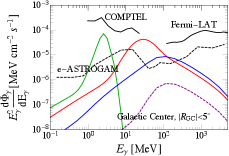
to plot the mass functions and gamma-ray spectra in Fig. 6. The shape of $\text{d}f_{\rm pbh}/\text{d}M$ is milder than the direct collapse scenario, and hence the gamma-ray spectra are much broader.

The accompanied GW signals can be calculated by $\{\alpha,\beta/H_{*},T_{*},v_{w}\}$ , as stated before Caprini:2015zlo ; Caprini:2019egz . In this scenario, the GWs peak at

f_{\rm peak}\approx 1.9\times 10^{-6}~{}{\rm Hz}\times\left(\frac{0.1}{v_{w}}\right)\left(\frac{\beta}{H_{*}}\right)\left(\frac{T_{*}}{{\rm GeV}}\right)\left(\frac{g_{*}}{100}\right)^{1/6},

(31)

where the normalized numbers are chosen according to the parameter scan described above. Unfortunately, this frequency region is not reachable by any current or future GW detectors. As illustrated in Fig. 7, the GW signals of the four BPs lie between the sensitive regions of the PTAs and the space-based interferometers, and this is also the general feature of the whole allowed parameter space. It is proposed that GWs with frequencies $\mu{\rm Hz}$ can be detected by future space-based $\mu$ Ares Sesana:2019vho or asteroid-based Fedderke:2021kuy interferometers, but there is still a long way to go to the final realization of those ideas. Therefore, the characteristic signal of the Fermi-ball collapse PBHs is that we can only see a mild gamma-ray spectrum, with no detected GWs. However, as implied by Eq. (29), the asteroid-mass PBHs in this mechanism favor a FOPT at GeV scale, which might be probed by BBN and CMB observations Bai:2021ibt ; Liu:2022lvz and show some correlation features with the PBH detection.

4 PBHs from cosmic strings

The spontaneous breaking of a $U(1)$ symmetry could form one-dimensional topological defects, known as the cosmic strings Nielsen:1973cs ; Kibble:1976sj ; Vachaspati:2015cma . When the symmetry is broken at a high scale $w$ , long string networks with a tension $\mu\sim w^{2}$ are formed. Those long strings are relativistic objects interacting and colliding frequently with themselves or each other, which continuously produces sub-horizon small string loops. The small loops then keep emitting GWs and shrinking until they disappear, generating the stochastic GW background today Auclair:2019wcv . A sub-horizon string may collapse into a PBH, if it shrinks to a size smaller than its Schwarzschild radius Hawking:1987bn ; Polnarev:1988dh . The fraction of cosmic strings that collapse into PBHs can be constrained by the gamma-rays from Hawking radiation Caldwell:1993kv ; MacGibbon:1997pu or CMB distortions James-Turner:2019ssu ; Bianchini:2022dqh .

Here we adopt the calculations in Refs. Caldwell:1993kv ; MacGibbon:1997pu ; James-Turner:2019ssu ; Caldwell:1991jj to derive the PBH mass function from cosmic string collapse. The energy density of the small string loops, $\rho_{\ell}$ , evolve as

\dot{\rho}_{\ell}+3H\rho_{\ell}=-\left[\dot{\rho}_{\infty}+2H\rho_{\infty}\left(1+\langle v^{2}\rangle\right)\right]\delta,

(32)

where $H=1/(2t)$ is the Hubble constant, $\rho_{\infty}$ is the energy density of long string networks, and numerical simulations show $\langle v^{2}\rangle\approx 0.4$ Blanco-Pillado:2011egf and $\delta\approx 0.1$ Blanco-Pillado:2013qja . The physical meaning of Eq. (32) is clear: small loops are being chopped off from the long strings, and hence a fraction of energy is transferred from the network system to the loop system. After reaching the scaling regime, $\rho_{\infty}\approx A\mu/(4t^{2})$ with $A\approx 44$ Blanco-Pillado:2011egf ; Blanco-Pillado:2019vcs . Therefore, the right-hand side of Eq. (32) is known. As for the left-hand side, $\rho_{\ell}=n_{\ell}\times\mu R_{\ell}$ , where $n_{\ell}$ is the number density of loops, $R_{\ell}$ is the length of an individual loop, which we assume to be a fixed fraction $\alpha_{\ell}\approx 0.1$ of the Hubble radius $H^{-1}=2t$ , i.e. $R_{\ell}=2\alpha_{\ell}t$ Blanco-Pillado:2011egf . If we further assume a fraction of $\epsilon$ of the small loops collapse into PBHs, then the number density of PBHs $n_{\rm pbh}=\epsilon\,n_{\ell}$ . Combining all information above, one obtains the evolution of PBH number density as

\dot{n}_{\rm pbh}+3Hn_{\rm pbh}=\epsilon\frac{A\delta}{8\alpha_{\ell}t^{4}}\left(1-\langle v^{2}\rangle\right).

(33)

The mass of PBH at time $t$ is $M\approx\mu\alpha_{\ell}t$ .

The PBHs from cosmic strings are mainly produced deep in the radiation era, as implied by Eq. (33). Integrating this equation up to the matter-radiation equality, we find

\frac{\text{d}f_{\rm pbh}}{\text{d}M}\Big{|}_{\rm eq}=\frac{\Omega_{m}}{\Omega_{\rm DM}}\left(\epsilon\frac{\alpha_{\ell}^{1/2}\mu^{3/2}A\delta}{8t_{\rm eq}^{3/2}}\frac{1-\langle v^{2}\rangle}{M^{3/2}}\right)\Big{/}\left(\frac{\pi^{2}}{30}g_{*}^{\rm eq}T_{\rm eq}^{4}\right).

(34)

taking into account the PBH evaporation, the mass function today is

\frac{\text{d}f_{\rm pbh}}{\text{d}M}=\left(\frac{M}{M^{\prime}}\right)^{3}\frac{\text{d}f_{\rm pbh}^{\rm eq}}{\text{d}M}\Big{|}_{M\to M^{\prime}},

(35)

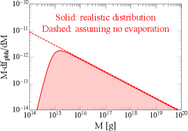
where $M^{\prime}=(M^{3}+3f_{0}M_{\rm Pl}^{4}t_{0})^{1/3}$ . Although Eq. (34) shows a $M^{-3/2}$ scaling, the evaporation effect makes current $\text{d}f_{\rm pbh}/\text{d}M\to 0$ for $M\lesssim 5\times 10^{14}$ g, as illustrated in the left panel of Fig. 8.

On the other hand, even though having evaporated, the light PBHs still leave impacts in the CMB. Ref. James-Turner:2019ssu reveals that the CMB anisotropies have constrained

\epsilon\lesssim 10^{-8}\left(\frac{0.1}{\delta}\right)\left(\frac{44}{A}\right)\left(\frac{0.1}{\alpha_{\ell}}\right)^{1/2}\left(\frac{0.6}{1-\langle v^{2}\rangle}\right)\left(\frac{10^{-15}}{G\mu}\right)^{3/2},

(36)

where

G\mu\equiv\frac{\mu}{M_{\rm Pl}^{2}}\sim 10^{-15}\left(\frac{w}{4\times 10^{11}~{}{\rm GeV}}\right)^{2}.

(37)

Note that Eq. (36) has set a constraint on $\epsilon\,\mu^{3/2}$ , which is also an overall factor of $\text{d}f_{\rm pbh}/\text{d}M$ , see Eq. (34). Since $\epsilon$ and $\mu$ are the only two free parameters in our simplified model, if we adopt the maximally allowed $\epsilon$ for a given $\mu$ , then $\text{d}f_{\rm pbh}/\text{d}M$ is already fixed. This can be treated as the largest cosmic string-induced PBH abundance allowed by current experiments.

We then evaluate the gamma-ray spectrum of the above PBH mass function. Unfortunately, as shown in the right panel of Fig. 8, it turns out that the gamma-ray signals are so weak that even future detectors cannot probe them. This conclusion is robust against the variation of $\epsilon$ and $\mu$ , as the shape is determined by the combination $\epsilon\,\mu^{3/2}$ , which is constrained by the CMB anisotropies James-Turner:2019ssu . But, as is well known, the stochastic GW background which has a flat strength at a large frequency range can be probed at future GW detectors, which might reach $G\mu\sim 10^{-18}$ Bian:2021vmi . Therefore, if the asteroid-mass PBHs are from cosmic string collapse, then we might detect the associated GW signals, but have no hope to see the direct gamma-ray signals due to their low abundance.

5 Summary and discussions

We summarize the main features of the four PBH scenarios in Table 1. One can see that they have qualitative different features originating from different physics in formation, and hence could be distinguished experimentally by combining the gamma-ray and GW signals. The asteroid-mass PBHs from cosmic strings are already constrained to have a very low abundance and their Hawking radiation signals are much smaller than indirect detection backgrounds. For the other three mechanisms, the gamma-rays are reachable at the e-ASTROGAM e-ASTROGAM:2016bph and AMEGO-X Fleischhack:2021mhc detectors which are proposed to be launched in the late 2020s. Solely using the gamma-ray signals, one can distinguish the “direct collapse during FOPT” scenario from the other two scenarios, as the corresponding PBHs have very sharp mass functions that yield sharp gamma-ray spectra. Furthermore, as the three mechanisms have very different associated GW signals, they can be clearly classified with the help of the future GW detectors built in 2030s. The summary plots of gamma-ray and GW signals are given in Fig. 9, where the first three scenarios use BP3 from Eq. (9), Eq. (24) and Eq. (30), respectively, and for the cosmic string scenario we choose $w=10^{13}$ GeV.

	Curvature perturbations	FOPT: direct collapse	FOPT: soliton collapse	Cosmic strings
Gamma-rays	Mild peak	Sharp peak	Mild peak	Not detectable
GW peak	$\mathcal{O}(1)$ Hz	$\mathcal{O}(10)$ Hz	$\mathcal{O}(10^{-6})$ Hz	Flat

Table 1: Signal features of different PBH formation mechanisms.

PBH has been a hot topic in both astrophysics and particle physics, and many different PBH formation mechanisms have been proposed in the past several decades. Our research provides a first systematic comparison of four well-motivated and extensively studied mechanisms, pointing out their own characteristic features in the asteroid-mass PBH region. We have demonstrated that with the new instruments in the next decade, we can hopefully not only detect asteroid-mass PBHs, but also identify their origins. Our work can be extended further. There are other mechanisms of forming PBHs, such as bubble collisions Hawking:1982ga ; Kodama:1982sf ; Moss:1994iq ; Konoplich:1999qq ; Kusenko:2020pcg ; Jung:2021mku or delayed vacuum decay Liu:2021svg ; Hashino:2021qoq ; He:2022amv ; Kawana:2022olo from a FOPT, or the collapse of domain walls Ferrer:2018uiu ; Ge:2019ihf ; Liu:2019lul , see the review Escriva:2022duf for more mechanisms. Studying the features of those other mechanisms and the possibility of identifying them in experiments would be interesting. Besides, other channels from multi-messenger astronomy, such as the $e^{\pm}$ and neutrinos from PBH evaporation, can be also used to pin down the PBH formation mechanism. We leave those studies for future work.

Acknowledgements.

We would like to thank Michael J. Baker, Anne M. Green, Joachim Kopp, and Tao Xu for the very useful and inspiring discussions. We are especially grateful to Tao Xu for communications on PBHs induced by curvature perturbations.

Appendix A Hawking Radiation and Gamma-ray spectrum

The huge gradient of the gravitational potential at the black hole horizon leads to particle production from the vacuum, which is known as the Hawking radiation process. The Hawking radiation could be described by the thermodynamics of a quasi-blackbody radiation spectrum, with an effective thermal temperature

T_{\rm pbh}=\frac{M_{\rm Pl}^{2}}{8\pi M}\approx 1.05~{}{\rm MeV}\times\left(\frac{10^{16}~{}{\rm g}}{M}\right),

(38)

which implies the dominant particles from the Hawking radiation of asteroid-mass PBHs are $\gamma$ , $e^{\pm}$ , $\mu^{\pm}$ , and $\pi^{\pm,0}$ . We assume only SM particles are produced by Hawking radiation. Recent studies found axion-like particles can also be produced and leave distinguishable features in gamma-ray spectra Agashe:2022phd ; Jho:2022wxd ; Li:2022mcf . The production of beyond SM particles does not change the conclusion of this study and we leave a dedicated spectrum analysis for the future.

The gravitational production rate of a particle species $i$ of mass $m_{i}$ in a logarithmic interval of energy $E_{i}$ is

\frac{\partial^{2}N_{i,{\rm pri}}}{\partial E_{i}\partial t}=\frac{g_{i}}{2\pi}\frac{\Gamma_{i}}{e^{E_{i}/T_{\rm pbh}}\pm 1},

(39)

where the subscript “pri” indicates this is the primary production, and $g_{i}$ is the degree of freedom of the emitted particle. The $+/-$ sign is taken for fermion/boson production. Although the Hawking radiation spectrum follows almost a blackbody shape, the existence of re-absorption at the black hole horizon causes a small modification on the low energy part of the energy spectrum. The deviation from a pure blackbody can be parametrized in the so-called graybody factor $\Gamma_{i}$ . The asymptotic approximation of graybody factor in the high energy limit $E_{i}\gg T_{\rm pbh}$ is $\Gamma_{i}=27G^{2}m^{2}_{i}E^{2}_{i}$ , while numerical methods are required to determine the re-absorption rate in the low energy region. One should note that the re-absorption rate varies for particles with different spins. We refer to the package BLACKHAWK Arbey:2019mbc ; Arbey:2021mbl for the value of $\Gamma_{i}$ for different particles’ spin and energy.

The gamma-ray spectrum from a PBH is contributed by the primary photons and the secondary photons from final state radiation (FSR) or decay of other primary particles. For the FSR from $e^{\pm}$ , $\mu^{\pm}$ and $\pi^{\pm}$ , there is

	$\displaystyle\frac{\text{d}N_{i\to i\gamma}}{\text{d}E_{\gamma}}$	$\displaystyle=$	$\displaystyle\frac{\alpha}{2\pi E_{i}}P_{i\rightarrow i\gamma}(x)\left[\log\left(\frac{1-x}{\mu_{i}^{2}}\right)-1\right],$		(40)
	$\displaystyle P_{i\rightarrow i\gamma}(x)$	$\displaystyle=$	$\displaystyle\begin{dcases}~{}\frac{2(1-x)}{x},&i=\pi^{\pm};\\ ~{}\frac{1+(1-x)^{2}}{x},&i=e^{\pm},~{}\mu^{\pm},\end{dcases}$		(41)

where $x=E_{\gamma}/E_{i}$ , $\mu_{i}=m_{i}/(2E_{i})$ . While for the decay from $\pi^{0}$ , one obtains

\frac{\text{d}N_{\pi^{0}\to\gamma\gamma}}{\text{d}E_{\gamma}}=\frac{\Theta(E_{\gamma}-E_{\pi^{0}}^{-})\Theta(E_{\pi^{0}}^{+}-E_{\gamma})}{E_{\pi^{0}}^{+}-E_{\pi^{0}}^{-}},\quad E_{\pi^{0}}^{\pm}=\frac{1}{2}\left(E_{\pi^{0}}\pm\sqrt{E_{\pi^{0}}^{2}-m_{\pi^{0}}^{2}}\right),

(42)

where $\Theta$ is the Heaviside function coming from the possible energy range of the final state photon. Summing up the above contributions, the total gamma-ray flux we have from a PBH is

\frac{\partial^{2}N_{\gamma}}{\partial E_{\gamma}\partial t}=\frac{\partial^{2}N_{\gamma,{\rm pri}}}{\partial E_{\gamma}\partial t}\\ +\sum_{i=e^{\pm},\mu^{\pm},\pi^{\pm}}\int\text{d}E_{i}\frac{\partial^{2}N_{i,{\rm pri}}}{\partial E_{i}\partial t}\frac{\text{d}N_{i\to i\gamma}}{\text{d}E_{\gamma}}+2\int\text{d}E_{\pi^{0}}\frac{\partial^{2}N_{\pi^{0},{\rm pri}}}{\partial E_{\pi^{0}}\partial t}\frac{\text{d}N_{\pi^{0}\to\gamma\gamma}}{\text{d}E_{\gamma}}.

(43)

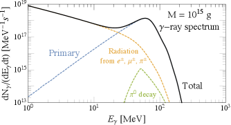
The total spectrum is illustrated in Fig. 10. Primary photon production is the most important contribution to the total photon spectrum, due to the highest flux and the direct relation between the photon spectrum peak and the PBH temperature.

With the gamma-ray production rate from a single PBH in Eq. (43), we can calculate the total gamma-ray flux from the target source. In this study, we focus on using an observation towards the galactic center. The gamma-ray flux $\Phi_{\gamma}$ at the earth can be calculated as

\begin{split}\frac{\text{d}\Phi_{\gamma}}{\text{d}E_{\gamma}}=&~{}\frac{\Delta\Omega}{4\pi}\times\left(\frac{1}{\Delta\Omega}\int_{\Delta\Omega}\text{d}\Omega\int_{\rm los}\text{d}l\,\rho_{\rm DM}\right)\int\frac{\text{d}M}{M}\frac{\text{d}f_{\rm pbh}}{\text{d}M}\frac{\partial^{2}N_{\gamma}}{\partial E_{\gamma}\partial t}\\ \equiv&~{}\frac{\Delta\Omega}{4\pi}J_{D}\int\frac{\text{d}M}{M}\frac{\text{d}f_{\rm pbh}}{\text{d}M}\frac{\partial^{2}N_{\gamma}}{\partial E_{\gamma}\partial t}.\end{split}

(44)

The $J_{D}$ is the D-factor of the galactic center for a ROI $\Delta\Omega$ . We choose $\Delta\Omega$ to be $|R_{\rm GC}|<5^{\circ}$ so that $\Delta\Omega=2.39\times 10^{-2}~{}{\rm sr}$ . For the distribution of local DM abundance, we use an NFW distribution for the Milky Way with as Navarro:1996gj

\rho_{\rm DM}(r)=\frac{\rho_{s}}{\frac{r}{r_{s}}\left(1+\frac{r}{r_{s}}\right)^{2}}.

(45)

The parameters of the NFW profile is taken from Table 3 of Ref. 2019JCAP…10..037D as $r_{s}=11~{}{\rm kpc}$ and $\rho_{{\rm DM},\odot}=0.376~{}{\rm GeV}/{\rm cm}^{3}$ , which we use to derive $\rho_{s}=0.839~{}{\rm GeV}/{\rm cm}^{3}$ . We use $r_{200}=193~{}{\rm kpc}$ to set the boundary of the galactic center halo for the line-of-sight (los) integral. In the end, we obtain the D-factor value $J_{D}=1.597\times 10^{26}~{}{\rm MeV}\cdot{\rm cm}^{-2}\cdot{\rm sr}^{-1}$ Coogan:2020tuf .

References

(1) Y. B. Zel’dovich and I. Novikov, “The hypothesis of cores retarded during expansion and the hot cosmological model,”Soviet Astronomy 10 (1967) 602.
(2) S. Hawking, “Gravitationally collapsed objects of very low mass,”Monthly Notices of the Royal Astronomical Society 152 (1971) 75–78.
(3) S. W. Hawking, “Black hole explosions,”Nature 248 (1974) 30–31.
(4) B. J. Carr, K. Kohri, Y. Sendouda and J. Yokoyama, “New cosmological constraints on primordial black holes,”Phys. Rev. D 81 (2010) 104019, [0912.5297].
(5) S. K. Acharya and R. Khatri, “CMB and BBN constraints on evaporating primordial black holes revisited,”JCAP 06 (2020) 018, [2002.00898].
(6) J. Chluba, A. Ravenni and S. K. Acharya, “Thermalization of large energy release in the early Universe,”Mon. Not. Roy. Astron. Soc. 498 (2020) 959–980, [2005.11325].
(7) T. Papanikolaou, V. Vennin and D. Langlois, “Gravitational waves from a universe filled with primordial black holes,”JCAP 03 (2021) 053, [2010.11573].
(8) T. Papanikolaou, “Gravitational waves induced from primordial black hole fluctuations: the effect of an extended mass function,”JCAP 10 (2022) 089, [2207.11041].
(9) T. Papanikolaou, C. Tzerefos, S. Basilakos and E. N. Saridakis, “Scalar induced gravitational waves from primordial black hole Poisson fluctuations in f(R) gravity,”JCAP 10 (2022) 013, [2112.15059].
(10) T. Papanikolaou, C. Tzerefos, S. Basilakos and E. N. Saridakis, “No constraints for $f(T)$ gravity from gravitational waves induced from primordial black hole fluctuations,” 2205.06094.
(11) B. Carr, K. Kohri, Y. Sendouda and J. Yokoyama, “Constraints on primordial black holes,”Rept. Prog. Phys. 84 (2021) 116902, [2002.12778].
(12) B. Carr and F. Kuhnel, “Primordial Black Holes as Dark Matter: Recent Developments,”Ann. Rev. Nucl. Part. Sci. 70 (2020) 355–394, [2006.02838].
(13) A. M. Green and B. J. Kavanagh, “Primordial Black Holes as a dark matter candidate,”J. Phys. G 48 (2021) 043001, [2007.10722].
(14) N. F. Bell and R. R. Volkas, “Mirror matter and primordial black holes,”Phys. Rev. D 59 (1999) 107301, [astro-ph/9812301].
(15) M. Y. Khlopov, A. Barrau and J. Grain, “Gravitino production by primordial black hole evaporation and constraints on the inhomogeneity of the early universe,”Class. Quant. Grav. 23 (2006) 1875–1882, [astro-ph/0406621].
(16) R. Allahverdi, J. Dent and J. Osinski, “Nonthermal production of dark matter from primordial black holes,”Phys. Rev. D 97 (2018) 055013, [1711.10511].
(17) O. Lennon, J. March-Russell, R. Petrossian-Byrne and H. Tillim, “Black Hole Genesis of Dark Matter,”JCAP 04 (2018) 009, [1712.07664].
(18) P. Gondolo, P. Sandick and B. Shams Es Haghi, “Effects of primordial black holes on dark matter models,”Phys. Rev. D 102 (2020) 095018, [2009.02424].
(19) I. Masina, “Dark matter and dark radiation from evaporating primordial black holes,”Eur. Phys. J. Plus 135 (2020) 552, [2004.04740].
(20) N. Bernal, F. Hajkarim and Y. Xu, “Axion Dark Matter in the Time of Primordial Black Holes,”Phys. Rev. D 104 (2021) 075007, [2107.13575].
(21) A. Cheek, L. Heurtier, Y. F. Perez-Gonzalez and J. Turner, “Primordial black hole evaporation and dark matter production. I. Solely Hawking radiation,”Phys. Rev. D 105 (2022) 015022, [2107.00013].
(22) A. Cheek, L. Heurtier, Y. F. Perez-Gonzalez and J. Turner, “Primordial black hole evaporation and dark matter production. II. Interplay with the freeze-in or freeze-out mechanism,”Phys. Rev. D 105 (2022) 015023, [2107.00016].
(23) P. Sandick, B. S. Es Haghi and K. Sinha, “Asymmetric reheating by primordial black holes,”Phys. Rev. D 104 (2021) 083523, [2108.08329].
(24) A. Cheek, L. Heurtier, Y. F. Perez-Gonzalez and J. Turner, “Evaporation of Primordial Black Holes in the Early Universe: Mass and Spin Distributions,” 2212.03878.
(25) D. Hooper, G. Krnjaic and S. D. McDermott, “Dark Radiation and Superheavy Dark Matter from Black Hole Domination,”JHEP 08 (2019) 001, [1905.01301].
(26) I. Masina, “Dark Matter and Dark Radiation from Evaporating Kerr Primordial Black Holes,”Grav. Cosmol. 27 (2021) 315–330, [2103.13825].
(27) A. Arbey, J. Auffinger, P. Sandick, B. Shams Es Haghi and K. Sinha, “Precision calculation of dark radiation from spinning primordial black holes and early matter-dominated eras,”Phys. Rev. D 103 (2021) 123549, [2104.04051].
(28) A. Cheek, L. Heurtier, Y. F. Perez-Gonzalez and J. Turner, “Redshift effects in particle production from Kerr primordial black holes,”Phys. Rev. D 106 (2022) 103012, [2207.09462].
(29) D. Toussaint, S. B. Treiman, F. Wilczek and A. Zee, “Matter - Antimatter Accounting, Thermodynamics, and Black Hole Radiation,”Phys. Rev. D 19 (1979) 1036–1045.
(30) M. S. Turner, “BARYON PRODUCTION BY PRIMORDIAL BLACK HOLES,”Phys. Lett. B 89 (1979) 155–159.
(31) A. F. Grillo, “Primordial Black Holes and Baryon Production in Grand Unified Theories,”Phys. Lett. B 94 (1980) 364–366.
(32) D. Baumann, P. J. Steinhardt and N. Turok, “Primordial Black Hole Baryogenesis,” hep-th/0703250.
(33) T. Fujita, M. Kawasaki, K. Harigaya and R. Matsuda, “Baryon asymmetry, dark matter, and density perturbation from primordial black holes,”Phys. Rev. D 89 (2014) 103501, [1401.1909].
(34) A. Hook, “Baryogenesis from Hawking Radiation,”Phys. Rev. D 90 (2014) 083535, [1404.0113].
(35) Y. Hamada and S. Iso, “Baryon asymmetry from primordial black holes,”PTEP 2017 (2017) 033B02, [1610.02586].
(36) L. Morrison, S. Profumo and Y. Yu, “Melanopogenesis: Dark Matter of (almost) any Mass and Baryonic Matter from the Evaporation of Primordial Black Holes weighing a Ton (or less),”JCAP 05 (2019) 005, [1812.10606].
(37) N. Bernal, C. S. Fong, Y. F. Perez-Gonzalez and J. Turner, “Rescuing high-scale leptogenesis using primordial black holes,”Phys. Rev. D 106 (2022) 035019, [2203.08823].
(38) D. Hooper and G. Krnjaic, “GUT Baryogenesis With Primordial Black Holes,”Phys. Rev. D 103 (2021) 043504, [2010.01134].
(39) Y. F. Perez-Gonzalez and J. Turner, “Assessing the tension between a black hole dominated early universe and leptogenesis,”Phys. Rev. D 104 (2021) 103021, [2010.03565].
(40) S. Datta, A. Ghosal and R. Samanta, “Baryogenesis from ultralight primordial black holes and strong gravitational waves from cosmic strings,”JCAP 08 (2021) 021, [2012.14981].
(41) S. Jyoti Das, D. Mahanta and D. Borah, “Low scale leptogenesis and dark matter in the presence of primordial black holes,”JCAP 11 (2021) 019, [2104.14496].
(42) T. C. Gehrman, B. Shams Es Haghi, K. Sinha and T. Xu, “Baryogenesis, Primordial Black Holes and MHz-GHz Gravitational Waves,” 2211.08431.
(43) LIGO Scientific, Virgo collaboration, B. P. Abbott et al., “Observation of Gravitational Waves from a Binary Black Hole Merger,”Phys. Rev. Lett. 116 (2016) 061102, [1602.03837].
(44) LIGO Scientific, Virgo collaboration, B. P. Abbott et al., “GW151226: Observation of Gravitational Waves from a 22-Solar-Mass Binary Black Hole Coalescence,”Phys. Rev. Lett. 116 (2016) 241103, [1606.04855].
(45) LIGO Scientific, VIRGO collaboration, B. P. Abbott et al., “GW170104: Observation of a 50-Solar-Mass Binary Black Hole Coalescence at Redshift 0.2,”Phys. Rev. Lett. 118 (2017) 221101, [1706.01812].
(46) S. Clesse and J. García-Bellido, “The clustering of massive Primordial Black Holes as Dark Matter: measuring their mass distribution with Advanced LIGO,”Phys. Dark Univ. 15 (2017) 142–147, [1603.05234].
(47) S. Bird, I. Cholis, J. B. Muñoz, Y. Ali-Haïmoud, M. Kamionkowski, E. D. Kovetz et al., “Did LIGO detect dark matter?,”Phys. Rev. Lett. 116 (2016) 201301, [1603.00464].
(48) M. Sasaki, T. Suyama, T. Tanaka and S. Yokoyama, “Primordial Black Hole Scenario for the Gravitational-Wave Event GW150914,”Phys. Rev. Lett. 117 (2016) 061101, [1603.08338].
(49) R. Bean and J. Magueijo, “Could supermassive black holes be quintessential primordial black holes?,”Phys. Rev. D 66 (2002) 063505, [astro-ph/0204486].
(50) M. Y. Khlopov, S. G. Rubin and A. S. Sakharov, “Primordial structure of massive black hole clusters,”Astropart. Phys. 23 (2005) 265, [astro-ph/0401532].
(51) N. Duechting, “Supermassive black holes from primordial black hole seeds,”Phys. Rev. D 70 (2004) 064015, [astro-ph/0406260].
(52) M. Kawasaki, A. Kusenko and T. T. Yanagida, “Primordial seeds of supermassive black holes,”Phys. Lett. B 711 (2012) 1–5, [1202.3848].
(53) S. Clesse and J. García-Bellido, “Massive Primordial Black Holes from Hybrid Inflation as Dark Matter and the seeds of Galaxies,”Phys. Rev. D 92 (2015) 023524, [1501.07565].
(54) V. De Luca, G. Franciolini and A. Riotto, “Clusteringenesis: from Light to Heavy Primordial Black Holes,” 2210.14171.
(55) S. Jung and T. Kim, “Gamma-ray burst lensing parallax: Closing the primordial black hole dark matter mass window,”Phys. Rev. Res. 2 (2020) 013113, [1908.00078].
(56) R. Laha, J. B. Muñoz and T. R. Slatyer, “INTEGRAL constraints on primordial black holes and particle dark matter,”Phys. Rev. D 101 (2020) 123514, [2004.00627].
(57) A. Coogan, L. Morrison and S. Profumo, “Direct Detection of Hawking Radiation from Asteroid-Mass Primordial Black Holes,”Phys. Rev. Lett. 126 (2021) 171101, [2010.04797].
(58) R. Laha, “Primordial Black Holes as a Dark Matter Candidate Are Severely Constrained by the Galactic Center 511 keV $\gamma$ -Ray Line,”Phys. Rev. Lett. 123 (2019) 251101, [1906.09994].
(59) W. DeRocco and P. W. Graham, “Constraining Primordial Black Hole Abundance with the Galactic 511 keV Line,”Phys. Rev. Lett. 123 (2019) 251102, [1906.07740].
(60) M. Boudaud and M. Cirelli, “Voyager 1 $e^{\pm}$ Further Constrain Primordial Black Holes as Dark Matter,”Phys. Rev. Lett. 122 (2019) 041104, [1807.03075].
(61) B. Dasgupta, R. Laha and A. Ray, “Neutrino and positron constraints on spinning primordial black hole dark matter,”Phys. Rev. Lett. 125 (2020) 101101, [1912.01014].
(62) A. Ray, R. Laha, J. B. Muñoz and R. Caputo, “Near future MeV telescopes can discover asteroid-mass primordial black hole dark matter,”Phys. Rev. D 104 (2021) 023516, [2102.06714].
(63) D. Ghosh, D. Sachdeva and P. Singh, “Future constraints on primordial black holes from XGIS-THESEUS,”Phys. Rev. D 106 (2022) 023022, [2110.03333].
(64) B. J. Carr and S. W. Hawking, “Black holes in the early Universe,”Mon. Not. Roy. Astron. Soc. 168 (1974) 399–415.
(65) B. J. Carr, “The Primordial black hole mass spectrum,”Astrophys. J. 201 (1975) 1–19.
(66) M. J. Baker, M. Breitbach, J. Kopp and L. Mittnacht, “Primordial Black Holes from First-Order Cosmological Phase Transitions,” 2105.07481.
(67) M. J. Baker, M. Breitbach, J. Kopp and L. Mittnacht, “Detailed Calculation of Primordial Black Hole Formation During First-Order Cosmological Phase Transitions,” 2110.00005.
(68) K. Kawana and K.-P. Xie, “Primordial black holes from a cosmic phase transition: The collapse of Fermi-balls,”Phys. Lett. B 824 (2022) 136791, [2106.00111].
(69) S. W. Hawking, “Black Holes From Cosmic Strings,”Phys. Lett. B 231 (1989) 237–239.
(70) K. Agashe, J. H. Chang, S. J. Clark, B. Dutta, Y. Tsai and T. Xu, “Correlating gravitational wave and gamma-ray signals from primordial black holes,”Phys. Rev. D 105 (2022) 123009, [2202.04653].
(71) e-ASTROGAM collaboration, A. De Angelis et al., “The e-ASTROGAM mission,”Exper. Astron. 44 (2017) 25–82, [1611.02232].
(72) H. Fleischhack, “AMEGO-X: MeV gamma-ray Astronomy in the Multi-messenger Era,”PoS ICRC2021 (2021) 649, [2108.02860].
(73) M. A. McLaughlin, “The North American Nanohertz Observatory for Gravitational Waves,”Class. Quant. Grav. 30 (2013) 224008, [1310.0758].
(74) NANOGRAV collaboration, Z. Arzoumanian et al., “The NANOGrav 11-year Data Set: Pulsar-timing Constraints On The Stochastic Gravitational-wave Background,”Astrophys. J. 859 (2018) 47, [1801.02617].
(75) K. Aggarwal et al., “The NANOGrav 11-Year Data Set: Limits on Gravitational Waves from Individual Supermassive Black Hole Binaries,”Astrophys. J. 880 (2019) 2, [1812.11585].
(76) A. Brazier et al., “The NANOGrav Program for Gravitational Waves and Fundamental Physics,” 1908.05356.
(77) R. N. Manchester et al., “The Parkes Pulsar Timing Array Project,”Publ. Astron. Soc. Austral. 30 (2013) 17, [1210.6130].
(78) R. M. Shannon et al., “Gravitational waves from binary supermassive black holes missing in pulsar observations,”Science 349 (2015) 1522–1525, [1509.07320].
(79) M. Kramer and D. J. Champion, “The European Pulsar Timing Array and the Large European Array for Pulsars,”Class. Quant. Grav. 30 (2013) 224009.
(80) L. Lentati et al., “European Pulsar Timing Array Limits On An Isotropic Stochastic Gravitational-Wave Background,”Mon. Not. Roy. Astron. Soc. 453 (2015) 2576–2598, [1504.03692].
(81) S. Babak et al., “European Pulsar Timing Array Limits on Continuous Gravitational Waves from Individual Supermassive Black Hole Binaries,”Mon. Not. Roy. Astron. Soc. 455 (2016) 1665–1679, [1509.02165].
(82) G. Hobbs et al., “The international pulsar timing array project: using pulsars as a gravitational wave detector,”Class. Quant. Grav. 27 (2010) 084013, [0911.5206].
(83) R. N. Manchester, “The International Pulsar Timing Array,”Class. Quant. Grav. 30 (2013) 224010, [1309.7392].
(84) J. P. W. Verbiest et al., “The International Pulsar Timing Array: First Data Release,”Mon. Not. Roy. Astron. Soc. 458 (2016) 1267–1288, [1602.03640].
(85) J. S. Hazboun, C. M. F. Mingarelli and K. Lee, “The Second International Pulsar Timing Array Mock Data Challenge,” 1810.10527.
(86) C. L. Carilli and S. Rawlings, “Science with the Square Kilometer Array: Motivation, key science projects, standards and assumptions,”New Astron. Rev. 48 (2004) 979, [astro-ph/0409274].
(87) G. Janssen et al., “Gravitational wave astronomy with the SKA,”PoS AASKA14 (2015) 037, [1501.00127].
(88) A. Weltman et al., “Fundamental physics with the Square Kilometre Array,”Publ. Astron. Soc. Austral. 37 (2020) e002, [1810.02680].
(89) LISA collaboration, P. Amaro-Seoane et al., “Laser Interferometer Space Antenna,” 1702.00786.
(90) TianQin collaboration, J. Luo et al., “TianQin: a space-borne gravitational wave detector,”Class. Quant. Grav. 33 (2016) 035010, [1512.02076].
(91) Y.-M. Hu, J. Mei and J. Luo, “Science prospects for space-borne gravitational-wave missions,”Natl. Sci. Rev. 4 (2017) 683–684.
(92) TianQin collaboration, J. Mei et al., “The TianQin project: current progress on science and technology,” 2008.10332.
(93) W.-R. Hu and Y.-L. Wu, “The Taiji Program in Space for gravitational wave physics and the nature of gravity,”Natl. Sci. Rev. 4 (2017) 685–686.
(94) W.-H. Ruan, Z.-K. Guo, R.-G. Cai and Y.-Z. Zhang, “Taiji program: Gravitational-wave sources,”Int. J. Mod. Phys. A 35 (2020) 2050075, [1807.09495].
(95) J. Crowder and N. J. Cornish, “Beyond LISA: Exploring future gravitational wave missions,”Phys. Rev. D 72 (2005) 083005, [gr-qc/0506015].
(96) S. Kawamura et al., “The Japanese space gravitational wave antenna: DECIGO,”Class. Quant. Grav. 28 (2011) 094011.
(97) LIGO Scientific, VIRGO collaboration, J. Aasi et al., “Characterization of the LIGO detectors during their sixth science run,”Class. Quant. Grav. 32 (2015) 115012, [1410.7764].
(98) LIGO Scientific, Virgo collaboration, B. P. Abbott et al., “Search for the isotropic stochastic background using data from Advanced LIGO’s second observing run,”Phys. Rev. D 100 (2019) 061101, [1903.02886].
(99) D. Reitze et al., “Cosmic Explorer: The U.S. Contribution to Gravitational-Wave Astronomy beyond LIGO,”Bull. Am. Astron. Soc. 51 (2019) 035, [1907.04833].
(100) M. Punturo et al., “The Einstein Telescope: A third-generation gravitational wave observatory,”Class. Quant. Grav. 27 (2010) 194002.
(101) S. Hild et al., “Sensitivity Studies for Third-Generation Gravitational Wave Observatories,”Class. Quant. Grav. 28 (2011) 094013, [1012.0908].
(102) B. Sathyaprakash et al., “Scientific Objectives of Einstein Telescope,”Class. Quant. Grav. 29 (2012) 124013, [1206.0331].
(103) P. Ivanov, P. Naselsky and I. Novikov, “Inflation and primordial black holes as dark matter,”Phys. Rev. D 50 (1994) 7173–7178.
(104) J. Garcia-Bellido, A. D. Linde and D. Wands, “Density perturbations and black hole formation in hybrid inflation,”Phys. Rev. D 54 (1996) 6040–6058, [astro-ph/9605094].
(105) J. Silk and M. S. Turner, “Double Inflation,”Phys. Rev. D 35 (1987) 419.
(106) M. Kawasaki, N. Sugiyama and T. Yanagida, “Primordial black hole formation in a double inflation model in supergravity,”Phys. Rev. D 57 (1998) 6050–6056, [hep-ph/9710259].
(107) J. Yokoyama, “Formation of MACHO primordial black holes in inflationary cosmology,”Astron. Astrophys. 318 (1997) 673, [astro-ph/9509027].
(108) S. Choudhury and A. Mazumdar, “Primordial blackholes and gravitational waves for an inflection-point model of inflation,”Phys. Lett. B 733 (2014) 270–275, [1307.5119].
(109) H. Di and Y. Gong, “Primordial black holes and second order gravitational waves from ultra-slow-roll inflation,”JCAP 07 (2018) 007, [1707.09578].
(110) S. Pi, Y.-l. Zhang, Q.-G. Huang and M. Sasaki, “Scalaron from $R^{2}$ -gravity as a heavy field,”JCAP 05 (2018) 042, [1712.09896].
(111) M. P. Hertzberg and M. Yamada, “Primordial Black Holes from Polynomial Potentials in Single Field Inflation,”Phys. Rev. D 97 (2018) 083509, [1712.09750].
(112) G. Ballesteros and M. Taoso, “Primordial black hole dark matter from single field inflation,”Phys. Rev. D 97 (2018) 023501, [1709.05565].
(113) R.-g. Cai, S. Pi and M. Sasaki, “Gravitational Waves Induced by non-Gaussian Scalar Perturbations,”Phys. Rev. Lett. 122 (2019) 201101, [1810.11000].
(114) I. Dalianis, A. Kehagias and G. Tringas, “Primordial black holes from $\alpha$ -attractors,”JCAP 01 (2019) 037, [1805.09483].
(115) O. Özsoy, S. Parameswaran, G. Tasinato and I. Zavala, “Mechanisms for Primordial Black Hole Production in String Theory,”JCAP 07 (2018) 005, [1803.07626].
(116) M. Cicoli, V. A. Diaz and F. G. Pedro, “Primordial Black Holes from String Inflation,”JCAP 06 (2018) 034, [1803.02837].
(117) B. Shams Es Haghi, “Baryogenesis and Primordial Black Hole Dark Matter from Heavy Metastable Particles,” 2212.11308.
(118) S. Choudhury, M. R. Gangopadhyay and M. Sami, “No-go for the formation of heavy mass Primordial Black Holes in Single Field Inflation,” 2301.10000.
(119) S. Bird, H. V. Peiris, M. Viel and L. Verde, “Minimally Parametric Power Spectrum Reconstruction from the Lyman-alpha Forest,”Mon. Not. Roy. Astron. Soc. 413 (2011) 1717–1728, [1010.1519].
(120) Planck collaboration, Y. Akrami et al., “Planck 2018 results. X. Constraints on inflation,”Astron. Astrophys. 641 (2020) A10, [1807.06211].
(121) J. C. Mather et al., “Measurement of the Cosmic Microwave Background spectrum by the COBE FIRAS instrument,”Astrophys. J. 420 (1994) 439–444.
(122) D. J. Fixsen, E. S. Cheng, J. M. Gales, J. C. Mather, R. A. Shafer and E. L. Wright, “The Cosmic Microwave Background spectrum from the full COBE FIRAS data set,”Astrophys. J. 473 (1996) 576, [astro-ph/9605054].
(123) J. Martin, H. Motohashi and T. Suyama, “Ultra Slow-Roll Inflation and the non-Gaussianity Consistency Relation,”Phys. Rev. D 87 (2013) 023514, [1211.0083].
(124) W. H. Kinney, “Horizon crossing and inflation with large eta,”Phys. Rev. D 72 (2005) 023515, [gr-qc/0503017].
(125) C. Germani and T. Prokopec, “On primordial black holes from an inflection point,”Phys. Dark Univ. 18 (2017) 6–10, [1706.04226].
(126) K. Dimopoulos, “Ultra slow-roll inflation demystified,”Phys. Lett. B 775 (2017) 262–265, [1707.05644].
(127) A. Riotto, “The Primordial Black Hole Formation from Single-Field Inflation is Not Ruled Out,” 2301.00599.
(128) S. Kawai and J. Kim, “Primordial black holes from Gauss-Bonnet-corrected single field inflation,”Phys. Rev. D 104 (2021) 083545, [2108.01340].
(129) S. Kawai and J. Kim, “CMB from a Gauss-Bonnet-induced de Sitter fixed point,”Phys. Rev. D 104 (2021) 043525, [2105.04386].
(130) S. Kawai and J. Kim, “Primordial black holes and gravitational waves from nonminimally coupled supergravity inflation,” 2209.15343.
(131) X. Wang, Y.-l. Zhang, R. Kimura and M. Yamaguchi, “Reconstruction of Power Spectrum of Primordial Curvature Perturbations on small scales from Primordial Black Hole Binaries scenario of LIGO/VIRGO detection,” 2209.12911.
(132) W. H. Press and P. Schechter, “Formation of galaxies and clusters of galaxies by selfsimilar gravitational condensation,”Astrophys. J. 187 (1974) 425–438.
(133) M. W. Choptuik, “Universality and scaling in gravitational collapse of a massless scalar field,”Phys. Rev. Lett. 70 (1993) 9–12.
(134) J. C. Niemeyer and K. Jedamzik, “Near-critical gravitational collapse and the initial mass function of primordial black holes,”Phys. Rev. Lett. 80 (1998) 5481–5484, [astro-ph/9709072].
(135) J. C. Niemeyer and K. Jedamzik, “Dynamics of primordial black hole formation,”Phys. Rev. D 59 (1999) 124013, [astro-ph/9901292].
(136) I. Musco, V. De Luca, G. Franciolini and A. Riotto, “Threshold for primordial black holes. II. A simple analytic prescription,”Phys. Rev. D 103 (2021) 063538, [2011.03014].
(137) A. Escrivà, “PBH Formation from Spherically Symmetric Hydrodynamical Perturbations: A Review,”Universe 8 (2022) 66, [2111.12693].
(138) Particle Data Group collaboration, P. A. Zyla et al., “Review of Particle Physics,”PTEP 2020 (2020) 083C01.
(139) S. Young, I. Musco and C. T. Byrnes, “Primordial black hole formation and abundance: contribution from the non-linear relation between the density and curvature perturbation,”JCAP 11 (2019) 012, [1904.00984].
(140) Fermi-LAT collaboration, M. Ackermann et al., “The Fermi Galactic Center GeV Excess and Implications for Dark Matter,”Astrophys. J. 840 (2017) 43, [1704.03910].
(141) S. C. Kappadath, Measurement of the Cosmic Diffuse Gamma-Ray Spectrum from 800 KEV to 30 Mev. PhD thesis, UNIVERSITY OF NEW HAMPSHIRE, Jan., 1998.
(142) R. Essig, E. Kuflik, S. D. McDermott, T. Volansky and K. M. Zurek, “Constraining Light Dark Matter with Diffuse X-Ray and Gamma-Ray Observations,”JHEP 11 (2013) 193, [1309.4091].
(143) K. Tomita, “Non-Linear Theory of Gravitational Instability in the Expanding Universe,”Progress of Theoretical Physics 37 (May, 1967) 831–846.
(144) S. Mollerach, D. Harari and S. Matarrese, “CMB polarization from secondary vector and tensor modes,”Phys. Rev. D 69 (2004) 063002, [astro-ph/0310711].
(145) K. N. Ananda, C. Clarkson and D. Wands, “The Cosmological gravitational wave background from primordial density perturbations,”Phys. Rev. D 75 (2007) 123518, [gr-qc/0612013].
(146) D. Baumann, P. J. Steinhardt, K. Takahashi and K. Ichiki, “Gravitational Wave Spectrum Induced by Primordial Scalar Perturbations,”Phys. Rev. D 76 (2007) 084019, [hep-th/0703290].
(147) V. Acquaviva, N. Bartolo, S. Matarrese and A. Riotto, “Second order cosmological perturbations from inflation,”Nucl. Phys. B 667 (2003) 119–148, [astro-ph/0209156].
(148) C. Yuan and Q.-G. Huang, “A topic review on probing primordial black hole dark matter with scalar induced gravitational waves,” 2103.04739.
(149) G. Domènech, “Scalar Induced Gravitational Waves Review,”Universe 7 (2021) 398, [2109.01398].
(150) S. Pi and M. Sasaki, “Gravitational Waves Induced by Scalar Perturbations with a Lognormal Peak,”JCAP 09 (2020) 037, [2005.12306].
(151) K. Kohri and T. Terada, “Semianalytic calculation of gravitational wave spectrum nonlinearly induced from primordial curvature perturbations,”Phys. Rev. D 97 (2018) 123532, [1804.08577].
(152) J. R. Espinosa, D. Racco and A. Riotto, “A Cosmological Signature of the SM Higgs Instability: Gravitational Waves,”JCAP 09 (2018) 012, [1804.07732].
(153) M. Braglia, D. K. Hazra, F. Finelli, G. F. Smoot, L. Sriramkumar and A. A. Starobinsky, “Generating PBHs and small-scale GWs in two-field models of inflation,”JCAP 08 (2020) 001, [2005.02895].
(154) K. Inomata, K. Kohri, T. Nakama and T. Terada, “Enhancement of Gravitational Waves Induced by Scalar Perturbations due to a Sudden Transition from an Early Matter Era to the Radiation Era,”Phys. Rev. D 100 (2019) 043532, [1904.12879].
(155) K. Inomata, M. Kawasaki, K. Mukaida, Y. Tada and T. T. Yanagida, “Inflationary primordial black holes for the LIGO gravitational wave events and pulsar timing array experiments,”Phys. Rev. D 95 (2017) 123510, [1611.06130].
(156) K. Inomata and T. Nakama, “Gravitational waves induced by scalar perturbations as probes of the small-scale primordial spectrum,”Phys. Rev. D 99 (2019) 043511, [1812.00674].
(157) J. Kozaczuk, T. Lin and E. Villarama, “Signals of primordial black holes at gravitational wave interferometers,”Phys. Rev. D 105 (2022) 123023, [2108.12475].
(158) M. Quiros, “Finite temperature field theory and phase transitions,” in ICTP Summer School in High-Energy Physics and Cosmology, pp. 187–259, 1, 1999. hep-ph/9901312.
(159) A. D. Linde, “Decay of the False Vacuum at Finite Temperature,”Nucl. Phys. B 216 (1983) 421.
(160) M. J. Baker, J. Kopp and A. J. Long, “Filtered Dark Matter at a First Order Phase Transition,”Phys. Rev. Lett. 125 (2020) 151102, [1912.02830].
(161) D. Chway, T. H. Jung and C. S. Shin, “Dark matter filtering-out effect during a first-order phase transition,”Phys. Rev. D 101 (2020) 095019, [1912.04238].
(162) W. Chao, X.-F. Li and L. Wang, “Filtered pseudo-scalar dark matter and gravitational waves from first order phase transition,”JCAP 06 (2021) 038, [2012.15113].
(163) X. Deng, X. Liu, J. Yang, R. Zhou and L. Bian, “Heavy dark matter and Gravitational waves,”Phys. Rev. D 103 (2021) 055013, [2012.15174].
(164) J.-P. Hong, S. Jung and K.-P. Xie, “Fermi-ball dark matter from a first-order phase transition,”Phys. Rev. D 102 (2020) 075028, [2008.04430].
(165) J. Arakawa, A. Rajaraman and T. M. P. Tait, “Annihilogenesis,”JHEP 08 (2022) 078, [2109.13941].
(166) P. Asadi, E. D. Kramer, E. Kuflik, G. W. Ridgway, T. R. Slatyer and J. Smirnov, “Accidentally Asymmetric Dark Matter,”Phys. Rev. Lett. 127 (2021) 211101, [2103.09822].
(167) P. Lu, K. Kawana and K.-P. Xie, “Old phase remnants in first-order phase transitions,”Phys. Rev. D 105 (2022) 123503, [2202.03439].
(168) K. Kawana, P. Lu and K.-P. Xie, “First-order phase transition and fate of false vacuum remnants,”JCAP 10 (2022) 030, [2206.09923].
(169) C. Caprini et al., “Science with the space-based interferometer eLISA. II: Gravitational waves from cosmological phase transitions,”JCAP 04 (2016) 001, [1512.06239].
(170) C. Caprini et al., “Detecting gravitational waves from cosmological phase transitions with LISA: an update,”JCAP 03 (2020) 024, [1910.13125].
(171) J. Ellis, M. Lewicki and J. M. No, “On the Maximal Strength of a First-Order Electroweak Phase Transition and its Gravitational Wave Signal,”JCAP 04 (2019) 003, [1809.08242].
(172) H.-K. Guo, K. Sinha, D. Vagie and G. White, “Phase Transitions in an Expanding Universe: Stochastic Gravitational Waves in Standard and Non-Standard Histories,”JCAP 01 (2021) 001, [2007.08537].
(173) J. R. Espinosa, T. Konstandin, J. M. No and G. Servant, “Energy Budget of Cosmological First-order Phase Transitions,”JCAP 06 (2010) 028, [1004.4187].
(174) D. Marfatia and P.-Y. Tseng, “Correlated signals of first-order phase transitions and primordial black hole evaporation,”JHEP 08 (2022) 001, [2112.14588].
(175) P. Huang and K.-P. Xie, “Primordial black holes from an electroweak phase transition,”Phys. Rev. D 105 (2022) 115033, [2201.07243].
(176) P.-Y. Tseng and Y.-M. Yeh, “511 keV galactic line from first-order phase transitions and primordial black holes,” 2209.01552.
(177) P. Lu, K. Kawana and A. Kusenko, “Late-Forming PBH: Beyond the CMB era,” 2210.16462.
(178) D. Marfatia and P.-Y. Tseng, “Boosted dark matter from primordial black holes produced in a first-order phase transition,” 2212.13035.
(179) D. E. Kaplan, M. A. Luty and K. M. Zurek, “Asymmetric Dark Matter,”Phys. Rev. D 79 (2009) 115016, [0901.4117].
(180) K. Petraki and R. R. Volkas, “Review of asymmetric dark matter,”Int. J. Mod. Phys. A 28 (2013) 1330028, [1305.4939].
(181) K. M. Zurek, “Asymmetric Dark Matter: Theories, Signatures, and Constraints,”Phys. Rept. 537 (2014) 91–121, [1308.0338].
(182) E. Krylov, A. Levin and V. Rubakov, “Cosmological phase transition, baryon asymmetry and dark matter Q-balls,”Phys. Rev. D 87 (2013) 083528, [1301.0354].
(183) F. P. Huang and C. S. Li, “Probing the baryogenesis and dark matter relaxed in phase transition by gravitational waves and colliders,”Phys. Rev. D 96 (2017) 095028, [1709.09691].
(184) Y. Bai, S. Lu and N. Orlofsky, “Origin of nontopological soliton dark matter: solitosynthesis or phase transition,”JHEP 10 (2022) 181, [2208.12290].
(185) E. Witten, “Cosmic Separation of Phases,”Phys. Rev. D 30 (1984) 272–285.
(186) J. A. Frieman and G. F. Giudice, “COSMIC TECHNICOLOR NUGGETS,”Nucl. Phys. B 355 (1991) 162–191.
(187) A. R. Zhitnitsky, “’Nonbaryonic’ dark matter as baryonic color superconductor,”JCAP 10 (2003) 010, [hep-ph/0202161].
(188) D. H. Oaknin and A. Zhitnitsky, “Baryon asymmetry, dark matter and quantum chromodynamics,”Phys. Rev. D 71 (2005) 023519, [hep-ph/0309086].
(189) K. Lawson and A. R. Zhitnitsky, “Isotropic Radio Background from Quark Nugget Dark Matter,”Phys. Lett. B 724 (2013) 17–21, [1210.2400].
(190) A. Atreya, A. Sarkar and A. M. Srivastava, “Reviving quark nuggets as a candidate for dark matter,”Phys. Rev. D 90 (2014) 045010, [1405.6492].
(191) Y. Bai and A. J. Long, “Six Flavor Quark Matter,”JHEP 06 (2018) 072, [1804.10249].
(192) Y. Bai, A. J. Long and S. Lu, “Dark Quark Nuggets,”Phys. Rev. D 99 (2019) 055047, [1810.04360].
(193) C. Gross, G. Landini, A. Strumia and D. Teresi, “Dark Matter as dark dwarfs and other macroscopic objects: multiverse relics?,”JHEP 09 (2021) 033, [2105.02840].
(194) A. Sesana et al., “Unveiling the gravitational universe at $\mu$ -Hz frequencies,”Exper. Astron. 51 (2021) 1333–1383, [1908.11391].
(195) M. A. Fedderke, P. W. Graham and S. Rajendran, “Asteroids for $\mu$ Hz gravitational-wave detection,”Phys. Rev. D 105 (2022) 103018, [2112.11431].
(196) Y. Bai and M. Korwar, “Cosmological constraints on first-order phase transitions,”Phys. Rev. D 105 (2022) 095015, [2109.14765].
(197) J. Liu, L. Bian, R.-G. Cai, Z.-K. Guo and S.-J. Wang, “Constraining first-order phase transitions with curvature perturbations,” 2208.14086.
(198) H. B. Nielsen and P. Olesen, “Vortex Line Models for Dual Strings,”Nucl. Phys. B 61 (1973) 45–61.
(199) T. W. B. Kibble, “Topology of Cosmic Domains and Strings,”J. Phys. A 9 (1976) 1387–1398.
(200) T. Vachaspati, L. Pogosian and D. Steer, “Cosmic Strings,”Scholarpedia 10 (2015) 31682, [1506.04039].
(201) P. Auclair et al., “Probing the gravitational wave background from cosmic strings with LISA,”JCAP 04 (2020) 034, [1909.00819].
(202) A. Polnarev and R. Zembowicz, “Formation of Primordial Black Holes by Cosmic Strings,”Phys. Rev. D 43 (1991) 1106–1109.
(203) R. R. Caldwell and E. Gates, “Constraints on cosmic strings due to black holes formed from collapsed cosmic string loops,”Phys. Rev. D 48 (1993) 2581–2586, [hep-ph/9306221].
(204) J. H. MacGibbon, R. H. Brandenberger and U. F. Wichoski, “Limits on black hole formation from cosmic string loops,”Phys. Rev. D 57 (1998) 2158–2165, [astro-ph/9707146].
(205) C. James-Turner, D. P. B. Weil, A. M. Green and E. J. Copeland, “Constraints on the cosmic string loop collapse fraction from primordial black holes,”Phys. Rev. D 101 (2020) 123526, [1911.12658].
(206) F. Bianchini and G. Fabbian, “CMB spectral distortions revisited: A new take on $\mu$ distortions and primordial non-Gaussianities from FIRAS data,”Phys. Rev. D 106 (2022) 063527, [2206.02762].
(207) R. R. Caldwell and B. Allen, “Cosmological constraints on cosmic string gravitational radiation,”Phys. Rev. D 45 (1992) 3447–3468.
(208) J. J. Blanco-Pillado, K. D. Olum and B. Shlaer, “Large parallel cosmic string simulations: New results on loop production,”Phys. Rev. D 83 (2011) 083514, [1101.5173].
(209) J. J. Blanco-Pillado, K. D. Olum and B. Shlaer, “The number of cosmic string loops,”Phys. Rev. D 89 (2014) 023512, [1309.6637].
(210) J. J. Blanco-Pillado, K. D. Olum and J. M. Wachter, “Energy-conservation constraints on cosmic string loop production and distribution functions,”Phys. Rev. D 100 (2019) 123526, [1907.09373].
(211) L. Bian, X. Liu and K.-P. Xie, “Probing superheavy dark matter with gravitational waves,”JHEP 11 (2021) 175, [2107.13112].
(212) S. W. Hawking, I. G. Moss and J. M. Stewart, “Bubble Collisions in the Very Early Universe,”Phys. Rev. D 26 (1982) 2681.
(213) H. Kodama, M. Sasaki and K. Sato, “Abundance of Primordial Holes Produced by Cosmological First Order Phase Transition,”Prog. Theor. Phys. 68 (1982) 1979.
(214) I. G. Moss, “Singularity formation from colliding bubbles,”Phys. Rev. D 50 (1994) 676–681.
(215) R. V. Konoplich, S. G. Rubin, A. S. Sakharov and M. Y. Khlopov, “Formation of black holes in first-order phase transitions as a cosmological test of symmetry-breaking mechanisms,”Phys. Atom. Nucl. 62 (1999) 1593–1600.
(216) A. Kusenko, M. Sasaki, S. Sugiyama, M. Takada, V. Takhistov and E. Vitagliano, “Exploring Primordial Black Holes from the Multiverse with Optical Telescopes,”Phys. Rev. Lett. 125 (2020) 181304, [2001.09160].
(217) T. H. Jung and T. Okui, “Primordial black holes from bubble collisions during a first-order phase transition,” 2110.04271.
(218) J. Liu, L. Bian, R.-G. Cai, Z.-K. Guo and S.-J. Wang, “Primordial black hole production during first-order phase transitions,”Phys. Rev. D 105 (2022) L021303, [2106.05637].
(219) K. Hashino, S. Kanemura and T. Takahashi, “Primordial black holes as a probe of strongly first-order electroweak phase transition,”Phys. Lett. B 833 (2022) 137261, [2111.13099].
(220) S. He, L. Li, Z. Li and S.-J. Wang, “Gravitational Waves and Primordial Black Hole Productions from Gluodynamics,” 2210.14094.
(221) K. Kawana, T. Kim and P. Lu, “PBH Formation from Overdensities in Delayed Vacuum Transitions,” 2212.14037.
(222) F. Ferrer, E. Masso, G. Panico, O. Pujolas and F. Rompineve, “Primordial Black Holes from the QCD axion,”Phys. Rev. Lett. 122 (2019) 101301, [1807.01707].
(223) S. Ge, “Sublunar-Mass Primordial Black Holes from Closed Axion Domain Walls,”Phys. Dark Univ. 27 (2020) 100440, [1905.12182].
(224) J. Liu, Z.-K. Guo and R.-G. Cai, “Primordial Black Holes from Cosmic Domain Walls,”Phys. Rev. D 101 (2020) 023513, [1908.02662].
(225) A. Escrivà, F. Kuhnel and Y. Tada, “Primordial Black Holes,” 2211.05767.
(226) K. Agashe, J. H. Chang, S. J. Clark, B. Dutta, Y. Tsai and T. Xu, “Detecting Axion-Like Particles with Primordial Black Holes,” 2212.11980.
(227) Y. Jho, T.-G. Kim, J.-C. Park, S. C. Park and Y. Park, “Axions from Primordial Black Holes,” 2212.11977.
(228) H.-J. Li, “Primordial black holes induced stochastic axion-photon oscillations in primordial magnetic field,”JCAP 11 (2022) 045, [2208.04605].
(229) A. Arbey and J. Auffinger, “BlackHawk: A public code for calculating the Hawking evaporation spectra of any black hole distribution,”Eur. Phys. J. C 79 (2019) 693, [1905.04268].
(230) A. Arbey and J. Auffinger, “Physics Beyond the Standard Model with BlackHawk v2.0,”Eur. Phys. J. C 81 (2021) 910, [2108.02737].
(231) J. F. Navarro, C. S. Frenk and S. D. M. White, “A Universal density profile from hierarchical clustering,”Astrophys. J. 490 (1997) 493–508, [astro-ph/9611107].
(232) P. F. de Salas, K. Malhan, K. Freese, K. Hattori and M. Valluri, “On the estimation of the local dark matter density using the rotation curve of the Milky Way,”jcap 2019 (Oct., 2019) 037, [1906.06133].