Pinned planar $p$-elasticae

For $p\in(1,\infty)$ and immersed curves $\gamma$ in the Euclidean plane $\mathbf{R}^{2}$, the $p$-bending energy is defined by

where $k$ denotes the signed curvature and $s$ denotes the arclength parameter of $\gamma$, respectively. A critical point of the $p$-bending energy under the fixed-length constraint is called $p$-elastica; in other words, its signed curvature is a (weak) solution to the Euler–Lagrange equation formally given by

where $\partial_{s}$ denotes the arclength derivative and $\lambda\in\mathbf{R}$ denotes a multiplier due to the fixed-length constraint. Classification of planar elasticae ($p=2$) is classic and given by Euler in the 18th century. Planar $p$-elasticae are just recently classified by the authors [19], with optimal regularity and closed formulae in terms of newly introduced $p$-elliptic functions. In particular, in the degenerate case $p>2$ the obtained family includes Watanabe’s flat-core solutions [28] (see also [25]), which are of qualitatively novel type compared to $p=2$. See [19] and references therein for details.

Boundary value problems for ($p$-)elasticae are in general more advanced because we need to detect the precise values of the multiplier or other geometric parameters for compatibility with the given boundary data, and thus need to solve the corresponding system of transcendental equations.

As a first step we focus on the so-called pinned boundary condition, which prescribes the endpoints up to zeroth order. More precisely, for given $P_{0},P_{1}\in\mathbf{R}^{2}$ and $L>0$ such that $|P_{0}-P_{1}|<L$, we define the admissible space by

where $\mathcal{L}$ denotes the length functional $\mathcal{L}[\gamma]:=\int_{\gamma}\,ds$, and $W^{2,p}_{\rm imm}(0,1;\mathbf{R}^{2})$ denotes the set of immersed $W^{2,p}$-curves:

We call a critical point of $\mathcal{B}_{p}$ in $\mathcal{A}_{P_{0},P_{1},L}$ pinned $p$-elastica (cf. Definition 2.11).

In the case of elastica ($p=2$) the pinned boundary value problem has been completely solved on the level of critical points and global minimizers [30, 17] (see also [15, 14, 1]). Roughly speaking, if $P_{0}=P_{1}$, then all pinned elasticae are part of “figure-eight”, while if $P_{0}\neq P_{1}$, then the curves are “arcs” and “loops” (like Figure 1). In any case, for given boundary data there are countably many critical points but the global minimizer is uniquely given by a “single arc” up to invariances.

Our primary result here extends the known classification of pinned planar elasticae for $p=2$ to all $p\in(1,\infty)$. In particular, in the degenerate case $p>2$, we find a critical distance of the endpoints at which the number of pinned $p$-elasticae changes from countable to uncountable. Following terminology in Definition 3.2, our result is summarized as follows (see also Figures 1 and 2).

Now we focus on global minimizers. Existence follows by a standard direct method. In addition, comparing the $p$-bending energy of all the above critical points, we obtain uniqueness of global minimizers.

A particularly useful case is where the endpoints agree $P_{0}=P_{1}$. In this case, by Theorems 1.1 and 1.4 we deduce that a half-fold (i.e., $\frac{1}{2}$-fold) figure-eight $p$-elastica is a unique global minimizer, extending [17, Proposition 2.6] from $p=2$ to $p\in(1,\infty)$ in the planar case. Here we apply this fact to obtain a Li–Yau type inequality and existence of minimal networks in the same spirit as [17]. In view of these applications it would be informative if we could know the precise geometric properties of the figure-eight $p$-elastica, in particular how the crossing angle depends on $p$. Fortunately we succeed in ensuring the following key monotonicity, cf. Figure 3:

This monotonicity is easy to infer from the numerical pictures but its analytic verification seems not straightforward. Our proof involves an indirect argument.

In what follows we discuss the aforementioned applications in detail. We also expect that our classification would be useful in other contexts, e.g. to detect the limit curves of gradient flows for the $p$-bending energy under the natural boundary condition. For recent developments of such flows, see e.g. [21, 22, 3, 4, 23].

We first apply our result to deduce a Li–Yau type inequality involving the normalized $p$-bending energy $\overline{\mathcal{B}}_{p}$, defined as the $p$-bending energy normalized by the length to be scale-invariant:

In their celebrated study, Li and Yau obtained the sharp inequality that the Willmore energy of a closed surface is bounded below by $4\pi$ times multiplicity [12]. A one-dimensional counterpart has also been studied by several authors [24, 27, 29, 20], and recently (almost) optimized in [17]: If an immersed closed $W^{2,2}$-curve $\gamma$ in $\mathbf{R}^{n}$ ($n\geq 2$) has a point of multiplicity $m\geq 2$, then

Here $\varpi^{*}>0$ denotes the normalized bending energy $\overline{\mathcal{B}}_{2}$ of a half-fold figure-eight elastica, and we say that a curve $\gamma$ has a point $P\in\mathbf{R}^{n}$ of multiplicity $m$ if the preimage $\gamma^{-1}(P)$ contains at least $m$ distinct points.

A typical characteristic of the 1D Li–Yau type inequality (compared to 2D) is the presence of a new algebraic obstruction for optimality of the inequality. In fact, it is proven in [17] that equality in (1.3) is attained if and only if $n\geq 3$ or $m$ is even, and also $\gamma$ is an $m$-leafed elastica. In particular, for $n=2$ and any odd multiplicity $m\geq 3$, the inequality is not optimal because of the irrationality of $\phi^{*}(2)/\pi$.

In this paper we first extend inequality (1.3) to all $p\in(1,\infty)$ in the plane, and then reveal some new phenomena on its optimality arising from the generality of $p$. Let $\mathbf{T}^{1}:=\mathbf{R}/\mathbf{Z}$ and $W^{2,p}_{\rm imm}(\mathbf{T}^{1};\mathbf{R}^{2})$ denote the set of immersed closed $W^{2,p}$-curves. Let $\varpi^{*}_{p}>0$ denote the normalized $p$-bending energy $\overline{\mathcal{B}}_{p}$ of a half-fold figure-eight $p$-elastica, which will be given by formula (5.1); in particular, $\varpi^{*}_{2}=\varpi^{*}$. Finally, we say that $\gamma$ is an $m$-leafed $p$-elastica if the curve $\gamma$ consists of $m$ half-fold figure-eight $p$-elasticae of same length (see Definition 5.3 for details). Then, applying Theorem 1.4, we establish the following

In addition, as in the case of $p=2$ [17], it is easy to see that if the multiplicity $m$ is even, then our inequality is always optimal.

As for odd multiplicity, the optimality is much more delicate (and does not hold for $p=2$ as discussed). However, for $p\neq 2$ we can apply Theorem 1.5 to find many new phenomena that recover optimality, even for closed planar curves with odd multiplicity. For example, there is a dense set $S\subset(1,\infty)$ such that each exponent $p\in S$ retrieves the optimality for all but a finite number of odd multiplicities (Theorem 5.11). In particular, as a very peculiar example, we discover a unique exponent for which inequality (1.4) becomes fully optimal.

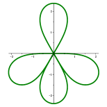
Moreover, for an odd $m\geq 3$, if we define $p_{m}:=(\phi^{*})^{-1}(\tfrac{\pi}{m})$, then the corresponding closed planar $m$-leafed $p_{m}$-elastica is unique (up to invariances) and has $m$-fold rotational symmetry, cf. Figure 4. These exponents can be used to ensure a “thresholding” phenomenon; for any given odd integer $2\ell+1\geq 3$ there is an exponent $p=p_{2\ell+1}$ for which optimality holds if and only if the multiplicity $m$ is none of $3,5,\dots,2\ell-1$ (see Theorem 5.12).

Another application is about existence of planar networks composed by three curves minimizing the normalized $p$-bending energy. Such a network structure is of recent interest particularly in geometric variational problems or flows as a model case with possible structural changes. See [2, 8, 6, 10, 7, 11, 21, 17] for some instances of static and dynamical studies of elastic networks.

In this paper, for given $\alpha\in(0,\pi)$, a triplet of immersed curves $(\gamma_{1},\gamma_{2},\gamma_{3})\in W^{2,p}_{\rm imm}(0,1;\mathbf{R}^{2})^{3}$ is called $\Theta$-network with angles $(\alpha,\alpha,2\pi-2\alpha)$ if $\gamma_{1}(0)=\gamma_{2}(0)=\gamma_{3}(0)$ and $\gamma_{1}(1)=\gamma_{2}(1)=\gamma_{3}(1)$, and if in addition the curves satisfy the angle condition

where we interpret $\gamma_{4}:=\gamma_{1}$. Let $\Theta(p,\alpha)$ denote the class of all $\Theta$-networks with angles $(\alpha,\alpha,2\pi-2\alpha)$, and for $\Gamma=(\gamma_{1},\gamma_{2},\gamma_{3})\in\Theta(p,\alpha)$ we define

where $\mathcal{L}[\Gamma]:=\sum_{i=1}^{3}\mathcal{L}[\gamma_{i}]$ and $\mathcal{B}_{p}[\Gamma]:=\sum_{i=1}^{3}\mathcal{B}_{p}[\gamma_{i}]$. Applying Theorems 1.4 and 1.5, we can obtain the existence of minimal $\Theta$-networks in a certain range of the angle $\alpha$:

In particular, focusing on the special “homogeneous” angle condition $\alpha={2\pi}/{3}$, we may rephrase Theorem 1.9 in terms of $p_{3}$ defined by (1.5).

Corollary 1.10 directly extends Dall’Acqua–Novaga–Pluda’s existence result for $p=2$ [7] (see also [17]) to $p>p_{3}$. Recall that numerically $p_{3}\simeq 1.5728$. Analytically we can ensure at least $p_{3}<2$ thanks to Theorem 1.5 with the fact that $\phi^{*}(2)<{\pi}/{3}=\phi^{*}(p_{3})$ (cf. [17, Lemma 3.11]).

In general, the existence of minimal elastic networks does not follow from a standard direct method due to the lack of compactness, namely the possibility that a component-curve degenerates into a point (see Section 6 for details). Our proof of Theorem 1.9 follows the general strategy of [17] strongly inspired by [7]. Although the proof in [7] contains a numerical part, the one in [17] gives a different analytic proof. Our proof here is also fully analytic. Along the way we establish and use new monotonicity results involving $p$-elliptic integrals.

We close the introduction by mentioning a few of many open problems. Concerning uniqueness of global minimizers, here we addressed the pinned boundary condition (Theorem 1.4), but as for the clamped boundary condition, only a few results are available even for $p=2$ (see e.g. [16] for the straightened case and [18] for the cuspidal case) and in particular it is widely open for $p\neq 2$ (except for the obvious closed case). Concerning the Li–Yau type inequality, the shape of a minimizer of $\overline{\mathcal{B}}_{p}$ among $W^{2,p}$-immersed closed planar curves with an odd multiplicity $m\geq 3$ is totally open unless equality in (1.4) is attained; in particular, if $p=2$, it is open for all odd $m\geq 3$. Finally, concerning minimal $p$-elastic networks, it is not clear whether the assumption $p>p_{3}$ in Corollary 1.10 (or (1.6) in Theorem 1.9) is optimal. We expect that the same existence result would not hold at least for $p$ sufficiently close to $1$, but even this is remained open.

This paper is organized as follows: In Section 2 we prepare notation and known results. In Section 3 we prove Theorem 1.1. In Section 4 we complete the proof of Theorems 1.4 and 1.5. Sections 5 and 6 are about applications to Li–Yau type inequalities and networks, respectively.

The first author is supported by JSPS KAKENHI Grant Numbers 18H03670, 20K14341, and 21H00990, and by Grant for Basic Science Research Projects from The Sumitomo Foundation. The second author is supported by JSPS KAKENHI Grant Number 22K20339.

Now we discuss some basic properties. As in the classical case $p=2$, the complete $p$-elliptic integrals $\mathrm{E}_{1,p}(q)$ and $\mathrm{K}_{1,p}(q)$ are not only monotone with respect to modulus $q\in[0,1)$ but also related by explicit derivative formulae:

In fact, the above derivative formulae are special cases of those for more general elliptic integrals obtained by Takeuchi [26]: For $a,b,c\in(1,\infty)$ and $q\in[0,1)$, let

By [26, Proposition 2], letting $c^{\prime}:={c}/{(c-1)}$ and $\xi:=1+{b}/{c}-{b}/{a}$, we have

We will also consider the ratio of the first and second complete $p$-elliptic integrals.

By this monotonicity of $Q_{p}$ we can define the unique modulus corresponding to “figure-eight”, which we will use frequently:

Next we recall the $p$-elliptic functions.

In addition, a typical part of $\operatorname{cn}_{p}(\cdot,1)$ and $\operatorname{dn}_{p}(\cdot,1)$ is interpreted as the $p$-hyperbolic secant function.

In general our $p$-elliptic functions satisfy fundamental properties such as periodicity and monotonicity similar to the classical Jacobian elliptic functions ($p=2$). In particular we recall some of those about $\operatorname{cn}_{p}$ and $\operatorname{sech}_{p}$ for later use.

Now we rigorously define pinned (planar) $p$-elasticae, and recall their known properties.

Let $\gamma$ be a pinned $p$-elastica. Then, by the Lagrange multiplier method (cf.  Proposition A.5), there is a multiplier $\lambda\in\mathbf{R}$ such that

for $h\in W^{2,p}(0,1;\mathbf{R}^{2})$ with $h(0)=h(1)=(0,0)$, where $D\mathcal{B}_{p}[\gamma]$ and $D\mathcal{L}[\gamma]$ are the Fréchet derivatives of $\mathcal{B}_{p}$ and $\mathcal{L}$ at $\gamma$, respectively. Using the arclength parameterization $\tilde{\gamma}$ of $\gamma$, we can rewrite (2.12) as

for $\eta\in W^{2,p}(0,L;\mathbf{R}^{2})$ with $\eta(0)=\eta(L)=(0,0)$ (cf. Proposition A.8). Moreover, we can translate (2.13) in terms of the signed curvature; indeed, according to [19, Proposition 2.1], if $\gamma\in W^{2,p}_{\rm imm}(0,1;\mathbf{R}^{2})$ satisfies (2.13), then its signed curvature $k:[0,L]\to\mathbf{R}$ (parameterized by the arclength) belongs to $L^{\infty}(0,L)$, and further $k$ satisfies

for all $\varphi\in W^{2,p}(0,L)$ with $\varphi(0)=\varphi(L)=0$ (although the class of test functions is different from [19], the derivation is parallel).

In particular, we find that any pinned $p$-elastica in the sense of Definition 2.11 is always a $p$-elastica in the sense of [19, Definition 1.1] by restricting test functions to $\eta\in C^{\infty}_{\rm c}(0,L;\mathbf{R}^{2})$ in (2.13). The complete classification of $p$-elasticae is already known. In order to state the classification, we prepare the notation on a concatenation of curves. For $\gamma_{j}:[a_{j},b_{j}]\to\mathbf{R}^{2}$ with $L_{j}:=b_{j}-a_{j}\geq 0$, we define $\gamma_{1}\oplus\gamma_{2}:[0,L_{1}+L_{2}]\to\mathbf{R}^{2}$ by

References

- [1] J. J. Arroyo, O. J. Garay, and A. Pámpano. Boundary value problems for Euler-Bernoulli planar elastica. A solution construction procedure. J. Elasticity, 139(2):359–388, 2020.
- [2] J. W. Barrett, H. Garcke, and R. Nürnberg. Elastic flow with junctions: variational approximation and applications to nonlinear splines. Math. Models Methods Appl. Sci., 22(11):1250037, 57, 2012.
- [3] S. Blatt, C. Hopper, and N. Vorderobermeier. A regularized gradient flow for the -elastic energy. Adv. Nonlinear Anal., 11(1):1383–1411, 2022.
- [4] S. Blatt, C. P. Hopper, and N. Vorderobermeier. A minimising movement scheme for the -elastic energy of curves. J. Evol. Equ., 22(2):Paper No. 41, 25, 2022.
- [5] T. Cazenave, D. Fang, and Z. Han. Continuous dependence for NLS in fractional order spaces. Ann. Inst. H. Poincaré C Anal. Non Linéaire, 28(1):135–147, 2011.
- [6] A. Dall’Acqua, C.-C. Lin, and P. Pozzi. Elastic flow of networks: long-time existence result. Geom. Flows, 4(1):83–136, 2019.
- [7] A. Dall’Acqua, M. Novaga, and A. Pluda. Minimal elastic networks. Indiana Univ. Math. J., 69(6):1909–1932, 2020.
- [8] A. Dall’Acqua and A. Pluda. Some minimization problems for planar networks of elastic curves. Geom. Flows, 2(1):105–124, 2017.
- [9] G. Del Nin, A. Pluda, and M. Pozzetta. Degenerate elastic networks. J. Geom. Anal., 31(6):6128–6170, 2021.
- [10] H. Garcke, J. Menzel, and A. Pluda. Willmore flow of planar networks. J. Differential Equations, 266(4):2019–2051, 2019.
- [11] H. Garcke, J. Menzel, and A. Pluda. Long time existence of solutions to an elastic flow of networks. Comm. Partial Differential Equations, 45(10):1253–1305, 2020.
- [12] P. Li and S. T. Yau. A new conformal invariant and its applications to the Willmore conjecture and the first eigenvalue of compact surfaces. Invent. Math., 69(2):269–291, 1982.
- [13] P. Lindqvist. Notes on the -Laplace equation (second edition). University Jyväskylä, Department of Mathematics and Statistics, Report 161, 2017.
- [14] A. Linnér. Explicit elastic curves. Ann. Global Anal. Geom., 16(5):445–475, 1998.
- [15] A. E. H. Love. A treatise on the Mathematical Theory of Elasticity. Dover Publications, New York, 1944. Fourth Ed.
- [16] T. Miura. Elastic curves and phase transitions. Math. Ann., 376(3-4):1629–1674, 2020.
- [17] T. Miura. Li–Yau type inequality for curves in any codimension, arXiv:2102.06597.
- [18] T. Miura, M. Müller, and F. Rupp. Optimal thresholds for preserving embeddedness of elastic flows. to appear in Amer. J. Math., arXiv:2106.09549.
- [19] T. Miura and K. Yoshizawa. Complete classification of planar -elasticae, arXiv:2203.08535v2.
- [20] M. Müller and F. Rupp. A Li-Yau inequality for the 1-dimensional Willmore energy. Adv. Calc. Var., 16(2):337–362, 2023.
- [21] M. Novaga and P. Pozzi. A second order gradient flow of -elastic planar networks. SIAM J. Math. Anal., 52(1):682–708, 2020.
- [22] S. Okabe, P. Pozzi, and G. Wheeler. A gradient flow for the -elastic energy defined on closed planar curves. Math. Ann., 378(1-2):777–828, 2020.
- [23] S. Okabe and G. Wheeler. The -elastic flow for planar closed curves with constant parametrization. J. Math. Pures Appl. (9), 173:1–42, 2023.
- [24] A. Polden. Curves and surfaces of least total curvature and fouth-order flows. PhD thesis, Universität Tübingen, 1996.
- [25] N. Shioji and K. Watanabe. Total -powered curvature of closed curves and flat-core closed -curves in . Comm. Anal. Geom., 28(6):1451–1487, 2020.
- [26] S. Takeuchi. Legendre-type relations for generalized complete elliptic integrals. J. Class. Anal., 9(1):35–42, 2016.
- [27] H. von der Mosel. Minimizing the elastic energy of knots. Asymptot. Anal., 18(1-2):49–65, 1998.
- [28] K. Watanabe. Planar -elastic curves and related generalized complete elliptic integrals. Kodai Math. J., 37(2):453–474, 2014.
- [29] G. Wheeler. On the curve diffusion flow of closed plane curves. Ann. Mat. Pura Appl. (4), 192(5):931–950, 2013.
- [30] K. Yoshizawa. The critical points of the elastic energy among curves pinned at endpoints. Discrete Contin. Dyn. Syst., 42(1):403–423, 2022.
- [31] E. Zeidler. Nonlinear functional analysis and its applications. III. Springer-Verlag, New York, 1985.
- [32] E. Zeidler. Nonlinear functional analysis and its applications. I. Springer-Verlag, New York, 1986.