Pinch-point spectral singularity from the interference of topological loop states
Abstract
Pinch point is a spectral discontinuity found in the neutron diffraction image of spin ice. Similar spectral singularity is commonly observed in a broad range of systems that have a close connection with flat bands. We focus on the electron flat band and its two topologically distinct classes of wavefunction: the compact localized state (CLS), and the non-contractible loop state (NLS). We establish their simple mathematical relationship, showing that different Bloch NLSs can be derived as momentum derivatives of a Bloch CLS, depending on the approaching direction toward the singular point. This CLS-NLS correspondence helps visualize the pinch point as an interference pattern among NLSs through a “polarizer”, which encodes the information about the location of singular momentum and the experimental techniques like spin-polarized photoemission spectroscopy. It helps extract topological information knit to microscopic electronic and magnetic structures.
Introduction. Characterization of quantum states using the language of topology often encounters difficulty in confirming it experimentally via local observables. One of the few exceptions to date is the integer quantum Hall systems [1] whose Hall conductivity is quantized in units of . In this light, the global loop states of flat bands may offer another example because they should have strong relevance to the observable singularity of the dynamical structure factor called pinch points.
The pinch point originally drew attention as a singularity of the magnetic structure factor of spin ice compounds, Ho2Ti2O7 [2, 3]. The spin ice state consists of a macroscopic number of classical states that satisfy a local constraint known as the ice rule, wherein the spin configuration within a tetrahedron sums to zero [4, 5]. From a field-theory point of view, the ice rule is a divergence-free condition in analogy with the divergence-free magnetic field lines in electromagnetism, which produces the algebraic dipolar spin correlation [6] and a resultant pinch point singularity at [7, 8]. However, pinch point is not a unique concept of spin ice.
The common origin of pinch points underlying a variety of systems is a flat band. It is known that the magnetic correlation of spin ice is accurately described within a large- approximation, which attributes the magnetic structure factor of spin ice to the flat band eigenfunctions in momentum space [7, 9, 8, 10]. This description offers two perspectives. Firstly, it highlights the ubiquity of pinch points in various systems ranging from frustrated magnets hosting classical spin liquids [11, 9, 12, 13, 14], tensor spin liquids [15], water ice [16, 17], ferroelectric models [18], to the materials with electronic flat bands [19, 20, 21, 22, 23, 24]. Secondly, there is a rich mathematical structure underlying the flat band eigenstates [25, 26, 27, 28, 29, 30, 31, 32, 33, 34, 27, 35, 36, 37, 38, 39] including global loop states [25, 26, 27, 28], quantum geometry [29, 30, 31, 32], and singularity at band-touching points [33]. Despite the knowledge accumulated on flat band and pinch point physics, their mutual relationship has not yet been clearly established.
Flat band phenomena. Let us illustrate what is known about flat bands using the kagome lattice. On the flat-band energy level, there exist states of at least the number of unit cells, . The absence of momentum dependence implies that these states can be written as localized states in real space, typically as the closed loops of finite length called a compact loop state (CLS).
Suppose that we have a single CLS state positioned at , denoted as , where one can generate its copies at by translation. By superposing them with a phase factor , one naturally expects that independent Bloch states constitute a flat band as
| (1) |
However, in a popular example of a tight-binding model on a kagome lattice, they fail to span a complete basis because (non-local constraint), resulting in only independent Bloch states in Eq. (1). The missing state is located at a momentum .
Bergmann et al. [26] identified these missing states as non-contractible loop states (NLS): a global loop state winding around the system, topologically different from CLS. The kagome lattice has two NLSs extending in different directions, and one of them complements the missing flat band state, whereas the other belongs to the dispersive band. The presence of two NLS ensures that the dispersive band touches the flat band at .
Indeed, the following facts on the “singular momentum” have been recursively discussed [40]; (i) vanishing norm of the CLS , (ii) existence of NLSs, (iii) the discontinuity of flat band wave functions, CLS () and NLS(), (iv) band touching, and (v) pinch point. Rhim and Yang referred to (i) - (iii) as different facets of the same physics, while they further showed counter-example; (iv) exists but (ii) and (iii) do not [28, 32]. There is a list of how the flat band phenomena like (ii) and (iv) are interpreted within a large- scheme in the classical spin liquid state of magnets [40]. Although (i)-(v) are commonly observed in flat band systems, their mutual relationships are not necessarily clear.
This Letter aims at establishing a simple relationship between NLS and CLS and make transparent connections among the aforementioned flat band phenomena. Through a consistent characterization, we can see how the pinch point spectrum arises from NLS interference, thereby enabling the extraction of topological information from observable pinch points.
Preliminaries. As the simplest platform, we consider a tight-binding Hamiltonian with nearest-neighbor hopping terms, , on kagome and pyrochlore lattices (Fig. 1(a)) for spatial dimensions, and , and number of sublattices, and , respectively. Let the lattice vector be given as with a unit vector in the -th direction, along which we impose periodic boundary conditions. The reciprocal lattice vectors satisfy . In kagome and pyrochlore lattices, sublattice vectors can be chosen as and for .
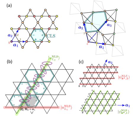
CLS-NLS correspondence. Let us continue with the kagome lattice. We may choose a primitive CLS around a hexagon as (Fig. 1(a)),
| (2) |
where denotes the electron state on the -th sublattice of the -th unit cell. Similarly, we can write down a single global NLS as
| (3) |
winding around a global loop in the direction 1(2)(Fig. 1(b)). Both CLS and NLS wavefunctions explicitly satisfy the divergence-free condition [41], i.e. the coefficients of sum to zero in each unit cell.
Once we choose an elementary CLS, its translation and superposition will provide a set of Bloch CLS,
| (4) | |||
| (8) |
In determining the vector, , the overlap of neighboring ’s, each spreading over a few unit cells, is essential. For example, is shared by two CLSs, and , and in the Bloch state , the former gives , while the latter, . Their sum yields in Eq. (8), where the factor appears because CLSs are shared in the direction 1. is also concerned with the norm of the Bloch CLS: . Then, at , where cannot be defined, i.e. gives a singular momentum.
We are now ready to introduce the CLS-NLS correspondence. The first observation on Eq. (4) is that if we replace the coefficient with one of its momentum derivatives, , and take , we find for example,
| (9) |
which is nothing but a Bloch NLS, i.e. the equal-weight superposition of the one-loop NLS (Eq. (3)) translated one by one in the direction . The factor is proportional to the weight of NLS state at sublattice . Similarly, the derivative results in another Bloch NLS , which superposes another one-loop NLS, , translated in the direction . To see why the -derivative can extract NLS from CLS, let us look at their relationships in Fig. 1(b). Along the one-loop NLS, , each site belonging to either or hinges two adjacent CLSs as marked with ovals. Acting on the phase factor assigned to these hinge sites, the -derivative extracts the one-loop NLS .
The second observation is that such -derivative naturally appears in the process of taking the limit, . To see this, we introduce the normalized Bloch CLS,
| (10) |
In approaching the singular point as and , the denominator vanishes linearly as . Given that , the coefficient of Eq. (10) approaches
| (11) |
Combing Eqs. (9) and (11), it is naturally shown that the Bloch NLS is obtained as the limit of normalized Bloch CLS. Because Eq. (11) means that different NLS state appears depending on the direction to approach , there is a discontinuity of flat band wavefunction at .
One can approach the singular point from an arbitrary direction as , and the Bloch CLS converges to a linearly combined two Bloch NLSs as
| (12) |
The simplest CLS-NLS correspondence, , is attained when approaching along the reciprocal vector, , where we have for , and for . They are the weight of sublattices constituting the associated one-loop NLS states, and , respectively (see Fig. 1(b)).
There might be a small complication in matching with due to the switch in indices, and . To explain this further, when approaching along , we find the NLS Bloch state consisting of loops, , running in direction 2, orthogonal to (). In other words, the loop regarded as a wavefront “propagates” in the direction 1 to form . Therefore, indexes the direction of the wavefront and not the winding direction of the loop state.
Degenerate flat bands at . We can generalize the above arguments to three and higher dimensions. One possible complication is the degeneracy of flat bands. Suppose the system has flat bands, then we can choose a set of linearly independent normalized Bloch CLS , with . If all these states simultaneously vanish at , this momentum is singular. In approaching along , each normalized Bloch CLS converges to a corresponding Bloch NLS, whose form , depends on the choice of . However, at least must live in the space orthogonal to , so that indexes the direction of the wavefront again, i.e. is the linear combination of one-loop NLS’s in the subspace spanned by the lattice vectors ’s, which satisfy .
As an example, we consider the pyrochlore lattice at , which hosts two-fold degenerate flat bands. As a counterpart of Eq. (8), we can choose two CLSs and , as their basis set, given as
| (21) |
each constructed from the primitive CLSs localized around hexagons on the sliced kagome plane, - and -, respectively (Fig 1 (a)). Both vanish at , that marks the singularity. For instance, in approaching along , the linear combination of normalized Bloch CLSs, , converges to the superposition of and winding along directions 1 and 2, and hence living on the [111] kagome plane orthogonal to 111See Sec. A in Supplemental Material. To see this, it is enough to notice , from Eq. (21), namely the two NLSs are placed on sublattices, .
From NLS to Pinch point. In diffraction measurements, we are concerned with the structure factor, which involves assessing the matrix element containing spatial details regarding sublattice coordinates. For example, in photoemission spectroscopy [43, 44, 45, 46], we are interested in the operator,
| (22) |
where creates an electron in the state . We now start from the electron ground state, , and examine the probability that one electron is added to the empty flat band state . The charge structure factor measured through the photoemission spectroscopy experiment is evaluated by the matrix element, , which can be rewritten using the normalized Bloch function, Eq. (10) as
| (23) | ||||
| (24) |
The vanishing of the norm, , gives the discontinuity of at , implying nothing but the pinch point singularity. This singularity potentially appears at a set of momenta, , shifted by arbitrary reciprocal vector , with integers . Whereas, the profile of may differ depending on , because the phase factor has different periodicities about 222The dependence of spectrum on phase factor is systematically studied by Conlon and Chalker [53] in different context..
Indeed, the profile is determined by the two factors that appear on the r.h.s. of Eq. (23). One factor is the vector and the other is the weight of the NLSs, . The former depends on the choice of but not on the approaching direction to , whereas for the latter the dependence is vice versa. The inner product of these two factors governs the profile of , indicating that the interference of independent NLSs occurs according to the selection rule encoded in . We call the vector “a polarizer” as it produces different images by varying the choice of NLSs when is translated by .
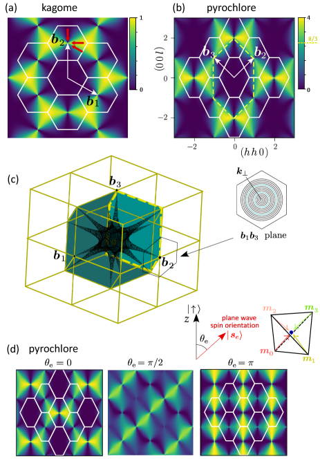
Examples. Revisiting the kagome lattice, we focus on the singular point , where the polarizer takes the form: . If we approach along (vertical line in Fig. 2(a)), the NLSs are chosen as , and vanishes as . Along , it yields . When approaching along a general direction, , only the component contributes according to Eq. (12), and takes a finite value. With these simple considerations we can reproduce a bowtie structure.
Even in the pyrochlore model with degenerate flat bands, we can identify the dark line where vanishes; we may target whose polarizer is . Approaching this point parallel to , NLSs have weights, , which is orthogonal to the polarizer and . This result is confirmed by the exact analytical form of given in Supplemental Material 333See Sec. B and Eq. (S16) in Supplemental Material. Figure 2(c) visualizes the low-intensity region, . This region develops around dark lines branching from the -point toward 12 different singular points, where the two dark cones touch.
Spin-dependent polarizer. One caveat is that the function of the polarizer depends on models and experimental probes. As an interesting case study, we consider the spin-polarized photoemission spectroscopy applied to the spin-orbit coupled flat band state on the pyrochlore lattice [49, 50]. Suppose we have a half-filled flat band in the ground state, with sublattice spins polarized as , where are the axes shown in Fig. 2(d). In the inverse photoemission spectroscopy to remove an electron from this ground state, the polarizer takes the form, , where stands for the spin state of the removed electron. Due to the additional spin-dependent matrix element , the dark line rotates with the spin orientation of the removed electron, , as shown in Fig. 2(d) 444See Sec. C in Supplemental Material. By carefully preparing a polarizer with dressed matrix elements, the information drawn from the spectrum can be used to clarify the microscopic spin structure of the state at focus.
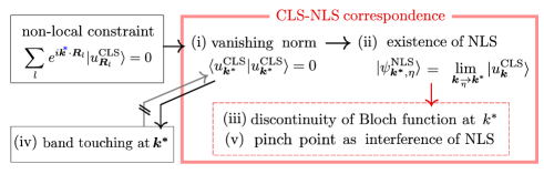
Summary and Discussion. We have established the CLS-NLS correspondence, identifying the Bloch NLS at the singular point as the momentum derivative of the Bloch CLS. The CLS-NLS correspondence makes a transparent connection among the flat band phenomena (i)-(v) as shown in Fig. 3. Here, (i) the vanishing of the norm of Bloch CLS enables the operation of momentum derivative in approaching the singular momentum, from which we reach the form of NLS in (ii) 555The combination of (i) and (ii) account for (iv) the presence of band touching [26, 28]. . NLS thus obtained is selected from among dependent choices, depending on the direction in approaching , which naturally explains (iii) the discontinuity of the flat band wavefunction. Finally, the NLS tomography around the singular momentum provides a simple way to describe (v) the structure of pinch point, as an interference pattern of the NLS.
To note, any flat bands including non-singular ones host CLSs, given a general construction [28], and supported by the arbitrarity of the choice of CLSs, “NLS” is derived from our formula. However, when CLSs span a complete flat band basis, such “NLS” is contractible and (ii) and (iii) break down. Band touching may occur in that case as well.
The CLS-NLS correspondence guarantees that we can always have NLS for singular flat bands, and can use it for identifying pinch points, or to extract from pinch points the electronic or magnetic structures of more complex systems with multi-degrees of freedom.
Although the system with perfect flat bands and ideal pinch point may seem to be a specific example, in reality there are a wide variety of materials with nearly flat bands in its vicinity. These classes of bands are allowed to host finite Chern numbers or may give another spectral feature known as half moons or “shadow pinch point” [53, 54, 55, 56, 57]. The variety of spectral patterns found there can be diagnosed using in a language of pinch points, and thus our CLS-NLS correspondence will provide a guiding principle to understand a broad range of systems close to flat band.
Acknowledgements.
H.N. was supported by a Grant-in-Aid for JSPS Research Fellow (Grant No. JP23KJ0783). This work is supported by KAKENHI Grant No. JP20H05655, JP21H05191, JP21K03440 and JP22H01147 from JSPS of Japan.References
- von Klitzing [1986] K. von Klitzing, Rev. Mod. Phys. 58, 519 (1986).
- Fennell et al. [2009] T. Fennell, P. P. Deen, A. R. Wildes, K. Schmalzl, D. Prabhakaran, A. T. Boothroyd, R. J. Aldus, D. F. McMorrow, and S. T. Bramwell, Science 326, 415 (2009).
- Kadowaki et al. [2009] H. Kadowaki, N. Doi, Y. Aoki, Y. Tabata, T. J. Sato, J. W. Lynn, K. Matsuhira, and Z. Hiroi, J. Phys. Soc. Jpn. 78, 103706 (2009).
- Udagawa and Jaubert [2021] M. Udagawa and L. Jaubert, eds., Spin Ice, Springer Series in Solid-State Sciences, Vol. 197 (Springer International Publishing, 2021).
- Bramwell and Gingras [2001] S. T. Bramwell and M. J. P. Gingras, Science 294, 1495 (2001).
- Huse et al. [2003] D. A. Huse, W. Krauth, R. Moessner, and S. L. Sondhi, Phys. Rev. Lett. 91, 167004 (2003).
- Isakov et al. [2004] S. V. Isakov, K. Gregor, R. Moessner, and S. L. Sondhi, Phys. Rev. Lett. 93, 167204 (2004).
- Henley [2005] C. L. Henley, Phys. Rev. B 71, 014424 (2005).
- Garanin and Canals [1999] D. A. Garanin and B. Canals, Phys. Rev. B 59, 443 (1999).
- Sen et al. [2013] A. Sen, R. Moessner, and S. L. Sondhi, Phys. Rev. Lett. 110, 107202 (2013).
- Moessner and Chalker [1998] R. Moessner and J. T. Chalker, Phys. Rev. Lett. 80, 2929 (1998).
- Canals and Garanin [2001] B. Canals and D. A. Garanin, Canadian Journal of Physics 79, 1323 (2001).
- Rehn et al. [2016] J. Rehn, A. Sen, K. Damle, and R. Moessner, Phys. Rev. Lett. 117, 167201 (2016).
- Benton and Moessner [2021] O. Benton and R. Moessner, Phys. Rev. Lett. 127, 107202 (2021).
- Prem et al. [2018] A. Prem, S. Vijay, Y.-Z. Chou, M. Pretko, and R. M. Nandkishore, Phys. Rev. B 98, 165140 (2018).
- Li et al. [1994] J. C. Li, V. M. Nield, D. K. Ross, R. W. Whitworth, C. C. Wilson, and D. A. Keen, Philosophical Magazine B 69, 1173 (1994).
- Isakov et al. [2015] S. V. Isakov, R. Moessner, S. L. Sondhi, and D. A. Tennant, Phys. Rev. B 91, 245152 (2015).
- Youngblood et al. [1980] R. Youngblood, J. D. Axe, and B. M. McCoy, Phys. Rev. B 21, 5212 (1980).
- Yan [2023] H. Yan, arXiv:2304.02204 (2023).
- Xie et al. [2019] Y. Xie, B. Lian, B. Jäck, X. Liu, C.-L. Chiu, K. Watanabe, T. Taniguchi, B. A. Bernevig, and A. Yazdani, Nature 572, 101 (2019).
- Mao et al. [2020] J. Mao, S. P. Milovanović, M. Anelković, X. Lai, Y. Cao, K. Watanabe, T. Taniguchi, L. Covaci, F. M. Peeters, A. K. Geim, Y. Jiang, and E. Y. Andrei, Nature 584, 215 (2020).
- Kang et al. [2020a] M. Kang, L. Ye, S. Fang, J.-S. You, A. Levitan, M. Han, J. I. Facio, C. Jozwiak, A. Bostwick, E. Rotenberg, M. K. Chan, R. D. McDonald, D. Graf, K. Kaznatcheev, E. Vescovo, D. C. Bell, E. Kaxiras, J. van den Brink, M. Richter, M. Prasad Ghimire, J. G. Checkelsky, and R. Comin, Nat. Mater. 19, 163 (2020a).
- Kang et al. [2020b] M. Kang, S. Fang, L. Ye, H. C. Po, J. Denlinger, C. Jozwiak, A. Bostwick, E. Rotenberg, E. Kaxiras, J. G. Checkelsky, and R. Comin, Nat. Commun. 11, 4004 (2020b).
- Lin et al. [2018] Z. Lin, J.-H. Choi, Q. Zhang, W. Qin, S. Yi, P. Wang, L. Li, Y. Wang, H. Zhang, Z. Sun, L. Wei, S. Zhang, T. Guo, Q. Lu, J.-H. Cho, C. Zeng, and Z. Zhang, Phys. Rev. Lett. 121, 096401 (2018).
- Sutherland [1986] B. Sutherland, Phys. Rev. B 34, 5208 (1986).
- Bergman et al. [2008] D. L. Bergman, C. Wu, and L. Balents, Phys. Rev. B 78, 125104 (2008).
- Maimaiti et al. [2017] W. Maimaiti, A. Andreanov, H. C. Park, O. Gendelman, and S. Flach, Phys. Rev. B 95, 115135 (2017).
- Rhim and Yang [2019] J.-W. Rhim and B.-J. Yang, Phys. Rev. B 99, 045107 (2019).
- Hwang et al. [2021a] Y. Hwang, J. Jung, J.-W. Rhim, and B.-J. Yang, Phys. Rev. B 103, L241102 (2021a).
- Hwang et al. [2021b] Y. Hwang, J.-W. Rhim, and B.-J. Yang, Phys. Rev. B 104, L081104 (2021b).
- Hwang et al. [2021c] Y. Hwang, J.-W. Rhim, and B.-J. Yang, Phys. Rev. B 104, 085144 (2021c).
- Rhim et al. [2020] J.-W. Rhim, K. Kim, and B.-J. Yang, Nature 584, 59 (2020).
- Rhim and Yang [2021] J.-W. Rhim and B.-J. Yang, Advances in Physics: X 6, 1901606 (2021).
- Miyahara et al. [2005] S. Miyahara, K. Kubo, H. Ono, Y. Shimomura, and N. Furukawa, J. Phys. Soc. Jpn. 74, 1918 (2005).
- Maimaiti et al. [2019] W. Maimaiti, S. Flach, and A. Andreanov, Phys. Rev. B 99, 125129 (2019).
- Mizoguchi and Udagawa [2019] T. Mizoguchi and M. Udagawa, Phys. Rev. B 99, 235118 (2019).
- Maimaiti et al. [2021] W. Maimaiti, A. Andreanov, and S. Flach, Phys. Rev. B 103, 165116 (2021).
- Essafi et al. [2017] K. Essafi, L. D. C. Jaubert, and M. Udagawa, J Phys Condens Matter 29, 315802 (2017).
- Bilitewski and Moessner [2018] T. Bilitewski and R. Moessner, Phys. Rev. B 98, 235109 (2018).
- Yan et al. [2023] H. Yan, O. Benton, A. H. Nevidomskyy, and R. Moessner, arXiv:2305.19189 (2023).
- Henley [2010] C. L. Henley, Annual Review of Condensed Matter Physics 1, 179 (2010).
- Note [1] See Sec. A in Supplemental Material.
- Damascelli et al. [2003] A. Damascelli, Z. Hussain, and Z.-X. Shen, Rev. Mod. Phys. 75, 473 (2003).
- Moser [2017] S. Moser, J. Electron Spectrosc. Relat. Phenom. 214, 29 (2017).
- Day et al. [2019] R. P. Day, B. Zwartsenberg, I. S. Elfimov, and A. Damascelli, npj Quantum Mater. 4, 54 (2019).
- Sobota et al. [2021] J. A. Sobota, Y. He, and Z.-X. Shen, Rev. Mod. Phys. 93, 025006 (2021).
- Note [2] The dependence of spectrum on phase factor is systematically studied by Conlon and Chalker [53] in different context.
- Note [3] See Sec. B and Eq. (S16) in Supplemental Material.
- Nakai and Hotta [2022] H. Nakai and C. Hotta, Nat. Commun. 13, 579 (2022).
- Nakai et al. [2023] H. Nakai, M. Kawano, and C. Hotta, Phys. Rev. B 108, L081106 (2023).
- Note [4] See Sec. C in Supplemental Material.
- Note [5] The combination of (i) and (ii) account for (iv) the presence of band touching [26, 28].
- Conlon and Chalker [2010] P. H. Conlon and J. T. Chalker, Phys. Rev. B 81, 224413 (2010).
- Udagawa et al. [2016] M. Udagawa, L. D. C. Jaubert, C. Castelnovo, and R. Moessner, Phys. Rev. B 94, 104416 (2016).
- Mizoguchi et al. [2017] T. Mizoguchi, L. D. C. Jaubert, and M. Udagawa, Phys. Rev. Lett. 119, 077207 (2017).
- Mizoguchi et al. [2018] T. Mizoguchi, L. D. C. Jaubert, R. Moessner, and M. Udagawa, Phys. Rev. B 98, 144446 (2018).
- Yan et al. [2018] H. Yan, R. Pohle, and N. Shannon, Phys. Rev. B 98, 140402 (2018).
- Okamoto et al. [2020] Y. Okamoto, H. Amano, N. Katayama, H. Sawa, K. Niki, R. Mitoka, H. Harima, T. Hasegawa, N. Ogita, Y. Tanaka, M. Takigawa, Y. Yokoyama, K. Takehana, Y. Imanaka, Y. Nakamura, H. Kishida, and K. Takenaka, Nature Communications 11, 3144 (2020).
Supplemental Material
.1 Convention of pyrochlore lattice and the choice of reciprocal lattice vectors
We take the lattice vectors of the pyrochlore lattice as , which gives shown in Fig. S1(a). In the pyrochlore lattice, we have four independent kagome planes which are denoted as , and by the vectors normal to these planes. If we construct a hexagonal CLS on the four species of hexagons on these planes, the four that share half of the edges and form a polygon are not independent of each other. Namely, the summation over them cancels out (see Fig. S1(b)). In this sense, only three of the four CLSs are linearly independent.
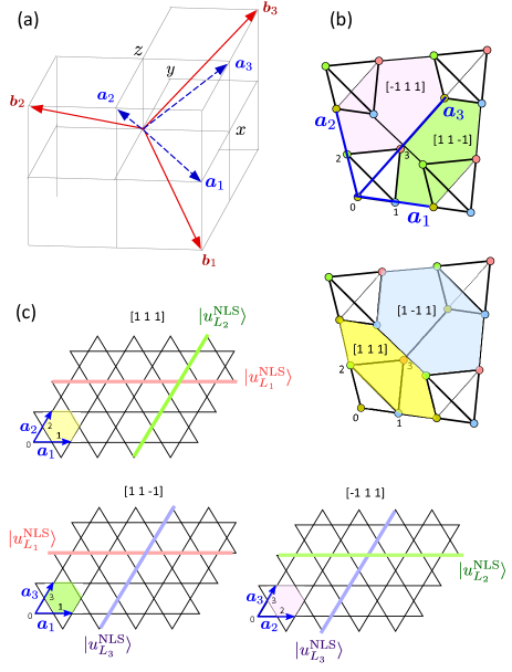
By using them we can construct a Bloch CLS confined within one sheet of kagome plane in each direction, as we do in the main text Eq. (4), which are shown schematically in Fig. S1(c) as colored hexagons. We can also visualize one-loop NLS on each plane. When we choose the kagome plane, the choices of three sublattices are , and we find two NLSs,
| (S1) |
which constitute the Bloch NLS, when approaching the singular point along .
Similarly, for the plane, we find one-loop NLSs,
| (S2) |
and for the plane,
| (S3) |
.2 Exact form of the spectral function
.2.1 general
If two or more flat bands exist, the formula of the structure factor must be generalized. The expression for the -fold degenerate flat bands takes the following form,
| (S4) |
Here, is the Gram matrix composed of the degenerate Bloch CLS bases, which are not necessarily orthogonal or normalized;
| (S5) |
is the sublattice component of the polarizer, and takes the form in the simplest case of photoemission spectroscopy, considered in the main text. If the flat band is not degenerate, the expression Eq. (S4), combined with Eq. (S5), is reduced to Eq. (12) in the main text.
.2.2 kagome lattice
Only a single flat band exists for the kagome lattice model. As written as Eq. (5) in the main text, the Bloch CLS takes the form,
| (S6) |
Putting this expression into Eq. (S4), we obtain
| (S7) |
By choosing the lattice coordinates, and , which gives and , we obtain as depicted in Fig. 2(a) in the main text.
.2.3 pyrochlore lattice
A pyrochlore lattice has two-fold degenerate flat bands (except for the spin degeneracy). The two basis vectors of Bloch CLS can be chosen as
| (S8) |
| (S9) |
and are respectively constructed from the primitive CLSs localized on kagome planes, and , as defined in Sec. .1.
.3 Spin-orbit coupled flat band states of the pyrochlore lattice
We introduce the spin-orbit coupled flat band model on a pyrochlore lattice [49, 50], which was originally introduced to address the exotic low-temperature insulating phase of CsW2O6 [58]. The tight-binding part of the model contains two parameters, spin-orbit coupling (SOC) and a standard transfer integral , and the Hamiltonian is written as
| (S17) |
with and . An SU(2) matrix rotates the electron spin by angle about the -axis when it hops from site to , and this angle varies with . Here, we take as an energy unit. When we have SOC flat bands.
In the SOC flat band state, the relative angle of spin orientation of the four sublattices is quenched while totally the SU(2) symmetry is kept. These spin configurations are given by setting a global spinor state and applying a set of operator , which is the rotation of the spins about the axis that points from the sublattice to the center of the tetrahedron, given as
| (S18) |
When we set pointing in the -direction of the pyrochlore -axis, the orientation of spins on four sublattices yields,
| (S23) |
where and are the zenithal and azimuthal angles of spins.
If finite Hubbard interaction is considered, the -electron ground state is still exactly obtained at quarter-filling for , where the lowest flat band is half occupied. The ground state can be written as
| (S24) |
where
| (S25) |
creates an electron at the -th flat band with the spin state . Here, the coefficients of flat band Bloch function, are chosen to be orthogonal to each other.
In the inverse spin-polarized photoemission spectroscopy, we take out one electron at the spin state . The corresponding matrix element is evaluated as
| (S26) |
where the creation operator of plane wave state is written as
| (S27) |
From Eqs. (S25) and (S27), we find
| (S28) |
The prefactor accounts for the polarizer in this case. We define the zenithal and azimuthal angles of incident spin as and set , and obtain the spectrum shown in Fig. 2(d) in the main text for , and .