Pileup corrections on higher-order cumulants

Let us first clarify the definition of the pileup events and assumptions to be made in the present study.

First, in experimental analyses the pileup events are removed using various methods, some of which are carried out by offline analysis. For example, suppose a correlation plot between number of particles measured by two detectors in different acceptances. The normal single-collision events are expected to appear as a band having a positive or negative slope. On the other hand, the pileup events would appear as additional bands having different slopes and/or offsets, while there could be be some uncorrelated components. The pileup events are then removed by cutting outlier events outside the correlated band. However, there will be a finite probability that the band is contaminated by the pileup events due to randomness. These events cannot be removed by this analysis. We call these residual events remaining after various cutting as the pile up events, and investigate the correction of their effects.

Second, in the following discussion two distribution functions play crucial roles. One of them is the “multiplicity distribution”, i.e. the distribution of the number of produced particles measured at mid- or forward-rapidity. The multiplicity is sometimes used to define centrality. The other distribution is the “particle distribution”. In the event-by-event analysis, we focus on the distribution of the number of a specific particle or charge, $N$, such as the net-proton number or net-charge, represented by the probability distribution function $P(N)$, and study its cumulants. Throughout this study, we consider the distribution of a single variable $N$ to simplify the discussion, but it is straightforward to extend the following method to deal with the multi-particle distributions, $P(N_{1},N_{2},\cdots)$, and the mixed cumulants of various particle species.

The distribution $P(N)$ depends on the multiplicity. Throughout this paper, we denote the experimentally-observed distribution function including the pileup effects at multiplicity $m$ as $P_{m}(N)$, while the distribution of $N$ in true single-collision events are represented as $P_{m}^{\rm t}(N)$. We suppose that $m$ and $N$ would be measured at different acceptances to reduce the auto-correlation effects between $m$ and $N$. This means that a collision event with $m=0$ can take place and have with nonzero $N$.

Third, except for Sec. II.3 we consider the pileup events composed of two single-collision events. As discussed in Sec. II.3, it is possible to extend the following analysis to include the pileup events with more than two single-collisions. The probability of those events, however, are usually well suppressed and explicit consideration of their effects are not needed. The important assumption taken throughout this paper is that two single-collision events included in a pileup event are independent.

Let us suppose that the pileup events occur with the probability $\alpha_{m}$ at the $m$th multiplicity bin. Then, the probability to find $N$ particles of interest at multiplicity $m$ with the pileup effects is given by

$\displaystyle P_{m}(N)$

$\displaystyle=$

$\displaystyle(1-\alpha_{m})P^{\rm t}_{m}(N)+\alpha_{m}{P}^{\rm pu}_{m}(N),$

(1)

where $P^{\rm t}_{m}(N)$ and $P^{\rm pu}_{m}(N)$ are the probability distribution functions of $N$ for the true (single-collision) and pileup events, respectively. The pileup events are further decomposed into the “sub-pileup” events given by the superposition of two single-collision events with multiplicities $i$ and $j$ satisfying $m=i+j$ as

	$\displaystyle P^{\rm pu}_{m}(N)$	$\displaystyle=$	$\displaystyle\sum_{i,j}\delta_{m,i+j}w_{i,j}P^{\rm sub}_{i,j}(N),$		(2)
	$\displaystyle P^{\rm sub}_{i,j}(N)$	$\displaystyle=$	$\displaystyle\sum_{N_{i},N_{j}}\delta_{N,N_{i}+N_{j}}P^{\rm t}_{i}(N_{i})P^{\rm t}_{j}(N_{j}),$		(3)

where $P^{\rm sub}_{i,j}(N)$ represents the probability distribution of $N$ in the sub-pileup events labeled by $(i,j)$, and $w_{i,j}$ is the probability to observe the sub-pileup events among the pileup events at the $m$th multiplicity bin. The sum over $i$ and $j$ runs non-negative integers. Obviously $w_{i,j}$ satisfies $w_{i,j}=w_{j,i}$ and

$\displaystyle\sum_{i,j}\delta_{m,i+j}w_{i,j}=1.$

(4)

From Eq. 4 one also finds $w_{0,0}=1$.

The pileup probabilities $\alpha_{m}$ and $w_{i,j}$ are related to the multiplicity distribution of the single-collision events. Let $T(m)$ be the multiplicity distribution, i.e. probability that a collision event with multiplicity $m$ occurs for all single-collision events. When all sub-pileup events are rejected by an experimental analysis with the same resolution, the probability to find a sub-pileup event labeled by $(i,j)$ among all collision events is given by $\alpha T(i)T(j)$, where $\alpha$ denotes the probability to find a pileup event among all collision events. Also, the probability to find an event with multiplicity $m$ without distinction between single-collision and pileup events is given by $(1-\alpha)T(m)+\alpha\sum_{i,j}\delta_{m,i+j}T(i)T(j)$. We thus have

	$\displaystyle w_{i,j}$	$\displaystyle=$	$\displaystyle\frac{\alpha T(i)T(j)}{\sum_{i,j}\delta_{m,i+j}\alpha T(i)T(j)},$		(5)
	$\displaystyle\alpha_{m}$	$\displaystyle=$	$\displaystyle\frac{\alpha\sum_{i,j}\delta_{m,i+j}T(i)T(j)}{(1-\alpha)T(m)+\alpha\sum_{i,j}\delta_{m,i+j}T(i)T(j)}.$		(6)

Therefore, in this case $\alpha_{m}$ and $w_{i,j}$ are completely determined from $\alpha$ and $T(m)$. We, however, note that Eqs. 5 and 6 might not hold in realistic experimental cases if the probability distribution of the pileup rejection is different from the multiplicity distribution. We thus do not use Eqs. 5 and 6 explicitly in the rest of this section. In real experiments, $w_{i,j}$ can directly be estimated by some reasonable assumptions within the experimental simulation. The models employed in Sec. III satisfy Eqs. 5 and 6.

From Eqs. 1, 2 and 3, the moment generating function Asakawa and Kitazawa (2016) for events at multiplicity $m$ is expressed as

	$\displaystyle G_{m}(\theta)$	$\displaystyle=$	$\displaystyle\sum_{N}e^{N\theta}P_{m}(N)$		(7)
		$\displaystyle=$	$\displaystyle(1-\alpha_{m})G^{\rm t}_{m}(\theta)+\alpha_{m}\sum_{i,j}\delta_{m,i+j}w_{i,j}G^{\rm sub}_{i,j}(\theta),$

with

$\displaystyle G^{\rm sub}_{i,j}(\theta)=G^{\rm t}_{i}(\theta)G^{\rm t}_{j}(\theta),$

(8)

where $G^{\rm t}_{m}(\theta)=\sum_{N}e^{N\theta}P^{\rm t}_{m}(N)$ is the moment generating function of $P_{m}^{\rm t}(N)$. The $r$th order moment of the observed distribution $P_{m}(N)$ is then given by

	$\displaystyle\langle N^{r}\rangle_{m}$	$\displaystyle=$	$\displaystyle\sum_{N}N^{r}P_{m}(N)=\frac{d^{r}}{d\theta^{r}}G(\theta)|_{\theta=0}$		(9)
		$\displaystyle=$	$\displaystyle(1-\alpha_{m})\langle N^{r}\rangle_{m}^{\rm t}+\alpha_{m}\sum_{i,j}\delta_{m,i+j}w_{i,j}\langle N^{r}\rangle_{i,j}^{\rm sub},$

with $\langle N^{r}\rangle_{m}^{\rm t}=\sum_{N}N^{r}P_{m}^{\rm t}(N)$ and

$\displaystyle\langle N^{r}\rangle_{i,j}^{\rm sub}$

$\displaystyle=$

$\displaystyle\sum_{N}N^{r}P_{i,j}^{\rm sub}(N)=\sum^{r}_{k=0}\binom{r}{k}\langle N^{r-k}\rangle_{i}^{\rm t}\langle N^{k}\rangle_{j}^{\rm t}.$

(10)

The right-hand sides in Eq. 10 up to fourth order are written as

	$\displaystyle\langle N\rangle_{i,j}^{\rm sub}$	$\displaystyle=$	$\displaystyle\langle N\rangle_{i}^{\rm t}+\langle N\rangle_{j}^{\rm t},$		(11)
	$\displaystyle\langle N^{2}\rangle_{i,j}^{\rm sub}$	$\displaystyle=$	$\displaystyle\langle N^{2}\rangle_{i}^{\rm t}+\langle N^{2}\rangle_{j}^{\rm t}+2\langle N\rangle_{i}^{\rm t}\langle N\rangle_{j}^{\rm t},$		(12)
	$\displaystyle\langle N^{3}\rangle_{i,j}^{\rm sub}$	$\displaystyle=$	$\displaystyle\langle N^{3}\rangle_{i}^{\rm t}+\langle N^{3}\rangle_{j}^{\rm t}+3\langle N^{2}\rangle_{i}^{\rm t}\langle N\rangle_{j}^{\rm t}+3\langle N\rangle_{i}^{\rm t}\langle N^{2}\rangle_{j}^{\rm t},$		(13)
	$\displaystyle\langle N^{4}\rangle_{i,j}^{\rm sub}$	$\displaystyle=$	$\displaystyle\langle N^{4}\rangle_{i}^{\rm t}+\langle N^{4}\rangle_{j}^{\rm t}+4\langle N^{3}\rangle_{i}^{\rm t}\langle N\rangle_{j}^{\rm t}+4\langle N\rangle_{i}^{\rm t}\langle N^{3}\rangle_{j}^{\rm t}+6\langle N^{2}\rangle_{i}^{\rm t}\langle N^{2}\rangle_{j}^{\rm t}.$		(14)

We note that Eq. 10 is alternatively expressed using cumulants in a compact form as Asakawa and Kitazawa (2016)

$$\langle N^{r}\rangle^{\rm sub}_{i,j,\rm c}=\langle N^{r}\rangle^{\rm t}_{i,\rm c}+\langle N^{r}\rangle^{\rm t}_{j,\rm c},$$

(15)

where $\langle N^{r}\rangle^{\rm sub}_{i,j,\rm c}$ and $\langle N^{r}\rangle^{\rm t}_{j,\rm c}$ are the cumulants of the sup-pileup and true distributions, respectively.

Substituting Eq. 10 into Eq. 9, one obtains formulas connecting $\langle N^{r}\rangle_{m}$ and $\langle N^{r}\rangle_{m}^{\rm t}$. It is notable that in these formulas the observed moment $\langle N^{r}\rangle_{m}$ is given by the combination of the true moments $\langle N^{r^{\prime}}\rangle_{m^{\prime}}^{\rm t}$ with $r^{\prime}\leq r$ and $m^{\prime}\leq m$.

The true moments $\langle N^{r}\rangle_{m}^{\rm t}$ are obtained from the observed moments $\langle N^{r}\rangle_{m}$ by solving Eqs. 9 and 10. This procedure can be carried out recursively starting from $m=0$ and $r=1$, and by increasing $m$ and $r$. To see this, it is convenient to rewrite Eqs. 9 and 10 as

$\displaystyle\langle N^{r}\rangle_{m}^{\rm t}$

$\displaystyle=$

$\displaystyle\cfrac{\langle N^{r}\rangle_{m}-\alpha_{m}C_{m}^{(r)}}{1-\alpha_{m}+2\alpha_{m}w_{m,0}},$

(16)

with

$\displaystyle C_{m}^{(r)}$

$\displaystyle=$

$\displaystyle\mu_{m}^{(r)}+\sum_{i,j>0}\delta_{m,i+j}w_{i,j}\langle N^{r}\rangle_{i,j}^{\rm sub},$

(17)

and

$\displaystyle\mu_{m}^{(r)}=\begin{cases}\displaystyle 2w_{m,0}\sum^{r-1}_{k=0}\binom{r}{k}\langle N^{r-k}\rangle_{0}^{\rm t}\langle N^{k}\rangle_{m}^{\rm t}&(m>0),\\ \displaystyle\sum^{r-1}_{k=1}\binom{r}{k}\langle N^{r-k}\rangle_{0}^{\rm t}\langle N^{k}\rangle_{0}^{\rm t}&(m=0).\end{cases}$

(18)

Up to the fourth order, the explicit forms of $\mu_{m}^{(r)}$ are

	$\displaystyle\mu_{m}^{(1)}$	$\displaystyle=$	$\displaystyle 0,$		(19)
	$\displaystyle\mu_{m}^{(2)}$	$\displaystyle=$	$\displaystyle 2w_{m,0}\left[\langle N^{2}\rangle_{0}^{\rm t}+2\langle N\rangle_{m}^{\rm t}\langle N\rangle_{0}^{\rm t}\right],$		(20)
	$\displaystyle\mu_{m}^{(3)}$	$\displaystyle=$	$\displaystyle 2w_{m,0}\left[\langle N^{3}\rangle_{0}^{\rm t}+3\langle N^{2}\rangle_{m}^{\rm t}\langle N\rangle_{0}^{\rm t}+3\langle N\rangle_{m}^{\rm t}\langle N^{2}\rangle_{0}^{\rm t}\right],$		(21)
	$\displaystyle\mu_{m}^{(4)}$	$\displaystyle=$	$\displaystyle 2w_{m,0}\left[\langle N^{4}\rangle_{0}^{\rm t}+4\langle N^{3}\rangle_{m}^{\rm t}\langle N\rangle_{0}^{\rm t}+4\langle N\rangle_{m}^{\rm t}\langle N^{3}\rangle_{0}^{\rm t}+6\langle N^{2}\rangle_{m}^{\rm t}\langle N^{2}\rangle_{0}^{\rm t}\right],$		(22)

for $m>0$ and

	$\displaystyle\mu_{0}^{(1)}$	$\displaystyle=$	$\displaystyle 0,$		(23)
	$\displaystyle\mu_{0}^{(2)}$	$\displaystyle=$	$\displaystyle 2\langle N_{0}\rangle^{\rm t}\langle N_{0}\rangle^{\rm t},$		(24)
	$\displaystyle\mu_{0}^{(3)}$	$\displaystyle=$	$\displaystyle 6\langle N_{0}^{2}\rangle^{\rm t}\langle N_{0}\rangle^{\rm t},$		(25)
	$\displaystyle\mu_{0}^{(4)}$	$\displaystyle=$	$\displaystyle 8\langle N_{0}^{3}\rangle^{\rm t}\langle N_{0}\rangle^{\rm t}+6\langle N_{0}^{2}\rangle^{\rm t}\langle N_{0}^{2}\rangle^{\rm t}.$		(26)

To obtain the true moments $\langle N^{r}\rangle_{m}^{\rm t}$, we first use the fact that $C_{0}^{(1)}=0$, which leads to $\langle N\rangle_{0}^{\rm t}=\langle N\rangle_{0}/(1+\alpha_{0})$. Next, Eqs. 17 and 18 shows that the correction factors $C_{0}^{(r)}$ at $m=0$ are given only by the moments $\langle N^{r^{\prime}}\rangle_{0}^{\rm t}$ with $r^{\prime}<r$. One thus can obtain $\langle N^{r}\rangle_{0}^{\rm t}$ recursively from lower order up to any higher orders. Similarly, one can obtain the true moments at multiplicity $m=1$ from lower order moments up to any order using the fact that the correction factor $C_{1}^{(r)}$ consists of $\langle N^{r^{\prime}}\rangle_{m^{\prime}}^{\rm t}$ with $r^{\prime}\leq r$ and $m^{\prime}\leq m$. By repeating the same procedure one can obtain the true moments for all multiplicities.

An important remark here is that this procedure can be carried out in almost data-driven way. Only thing we need is the probabilities $w_{i,j}$ and $\alpha_{m}$, which would be determined by simulations.

So far, we considered the pileup events composed of two single-collision events. It is not difficult to extend these results to include the pileup events composed of three single-collision events. In this case, Eq. 2 is modified as

$\displaystyle P_{m}^{\rm pu}=\sum_{i,j}\delta_{m,i+j}w_{i,j}P_{i,j}^{\rm sub}(N)+\sum_{i,j,k}\delta_{m,i+j+k}w_{i,j,k}P_{i,j,k}^{\rm sub}(N),$

(27)

where $P_{i,j,k}^{\rm sub}(N)$ represents the probability distribution of $N$ on the sub-pileup events composed of three single collisions with multiplicities $i$, $j$, and $k$, and $w_{i,j,k}$ is the probability of the sub-pileup event. From the independence of the individual collisions, $P_{i,j,k}^{\rm sub}(N)$ is given by

$\displaystyle P_{i,j,k}^{\rm sub}=\sum_{N_{i},N_{j},N_{k}}\delta_{N,N_{i}+N_{j}+N_{k}}P_{i}^{\rm t}(N_{i})P_{j}^{\rm t}(N_{j})P_{j}^{\rm t}(N_{j}).$

(28)

Then, it is straightforward to derive the relations like Eqs. 9 and 16. These results allow us to obtain the true moments $\langle N^{r}\rangle_{m}^{\rm t}$ recursively from small $m$ as before. In this way, pileups with arbitrary many single-collision events can be taken into account in principle.

Let us first generate a realistic multiplicity distribution with pileup events. We employ the Glauber and two-component model for this purpose. Two gold nuclei are collided in the Glauber model, where the $pp$ cross section is chosen to be $33$ mb. The number of participant nucleons, $N_{\rm part}$, and binary collisions, $N_{\rm coll}$, are obtained. In order to propagate $N_{\rm part}$ and $N_{\rm coll}$ to the multiplicity, we define the number of sources, $N_{\rm sc}$ as

$\displaystyle N_{\rm sc}=(1-x)N_{\rm part}+xN_{\rm coll},$

(29)

where $x$ is the fraction of the hard component. We choose $x=0.1$ for the simulation. Particles are then generated from each source $N_{\rm sc}$ based on the negative binomial distribution:

$\displaystyle P_{\mu,k}(N)=\cfrac{\Gamma(N+k)}{\Gamma(N+1)\Gamma(k)}\cdot\cfrac{(\mu/k)^{N}}{(\mu/k+1)^{N+k}},$

(30)

where $\mu$ is the mean value of particles generated from one source, and $k$ corresponds to the inverse of width of the distribution. $\mu=1.0$ and $k=1.0$ are chosen for the simulation. In order to simulate the pileup events as well as normal single-collision events, multiplicities from two collision events are randomly superimposed with the probability $\alpha=0.05$. In this way, 10 million Au+Au collision events are processed. We note that in this model the pileup probabilities $w_{i,j}$ and $\alpha_{m}$ are given by Eqs. 5 and 6 by construction.

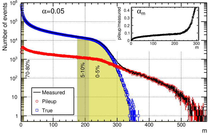
The resulting multiplicity distribution is shown by the black line in Fig. 1. The blue squares show the multiplicity distribution from single-collision events, while those from pileup events are shown by the red circles. It is found that, due to the pileup events, the measured distribution has the tail on top of the distribution from the single-collision events. The inset panel shows $\alpha_{m}$, i.e. the ratio of the pileup events at multiplicity $m$. From the panel one finds that $\alpha_{m}$ grows with increasing $m$. This behavior suggests that the effect of pileup events are more problematic in central collisions rather than peripheral collisions.

In Fig. 2, we plot the multiplicity distribution of single-collision events $T(m)$ and the number of sub-pileup events $(i,j)$ normalized by total simulated events, $\alpha T(i)T(j)$. From these results $w_{i,j}$ and $\alpha_{m}$ are constructed according to Eqs. 5 and 6. These parameters are used in the following two subsections.

In this and next subsections, we discuss the pileup correction for two model distributions $P_{m}^{\rm t}(N)$ with the multiplicity distribution obtained in Sec. III.1. In this subsection, we consider a simple model where the particle number $N$ obeys the Poisson distribution with the mean value of $10$ at all the multiplicity bin. We emphasize that this model is totally impractical, because $10$ particles on average are created at both $m=0$ and $m=300$. However, this model is suitable to demonstrate the validity of the recursive correction procedures. The more realistic model will be discussed in the next subsection.

Figure 3 shows the particle distribution for the first 4 multiplicity bins ($m=0$, 1, 2, 3). The red circles show pileup events, and the blue squares show the single-collision events. The measured distribution given by the sum of these distributions is shown by the black solid lines, which are found to have a bump structure at $N\gtrsim 20$ due to pileup events. Other colored lines show the sub-pileup events for all possible combinations of ($i$,$j$) with $m=i+j$. In the case of $m=0$, there is only one combination for sub-pileup, $(i,j)=(0,0)$, and the distributions of pileup and sub-pileup events are identical and $w_{0,0}=1$. As shown in Fig. 3 (b), (c) and (d), in the case of $m\geq 1$, the pileup distribution consists of multiple sub-pileup events with $(i,j)=(m,0)$, $\cdots$, $(0,m)$.

In Fig. 4, we show the cumulants $\langle N^{r}\rangle_{m,\rm c}$ at the $m$th multiplicity bin. In the figure, the cumulants are plotted for the true single-collision distribution obtained by the simulation, measured distribution with the pileup effects, and the corrected results. Statistical uncertainties are estimated by bootstrap. True cumulants are $\langle N^{r}_{m}\rangle=10$ by definition. The measured cumulants have strong deviations from this value due to the pileup events Sombun et al. (2018); Garg and Mishra (2017). It is notable that the measured cumulants especially for $r=1$ and 2 behave similar to what we have already seen in $\alpha_{m}$ in the inset panel in Fig. 1. Because the particles are generated according to the Poisson distributions having the same mean value, the effects from the pileup events only depend on the pileup probability. Corrected cumulants are found to be consistent with the true value $\langle N^{r}\rangle_{m,\rm c}=10$ within statistics, which indicates that our method does work well. Large point-by-point variations are due to the increased statistical uncertainties after the corrections.

Next, we move on to more realistic case, where the mean value of $N$ increases with increasing $N_{\rm part}$. We again employ the Poisson distribution for $N$, but in contrast to the previous subsection we assume that the mean value varies depending on $N_{\rm part}$ as $\langle N\rangle=0.05N_{\rm part}$. We employ the same pileup probability $\alpha=0.05$. The centrality is defined by dividing the multiplicity distribution of single-collision events (see Fig. 1 for corresponding regions in multiplicity distributions). Figure 5 shows the particle number distributions for 0-5%, 10-20%, 40-50% and 70-80% centralities. The pileup distributions are found inside the true distribution at peripheral collisions, while the pileup distributions in central collisions appear as a long tail in the measured distributions. Thus, large effects on cumulants are expected in central collisions in this simulation Garg and Mishra (2017).

Cumulants for each multiplicity bin are averaged in each centrality by using event statistics as a weight Luo and Xu (2017), which are shown in Fig. 6 as a function of centrality. The centrality is $0-5\%$, $5-10\%$, $10-20\%$… ,$70-80\%$ from $x=0$ to $x=8$. In this case, significant deviation on measured cumulants are observed only in the central collisions, as was expected from Fig. 5. Corrected cumulants are consistent with true cumulants even at $0-5\%$. This result shows that the pileup correction proposed in Sec. II is successfully applicable to realistic particle distributions.

It would be interesting to discuss briefly about volume fluctuations Skokov et al. (2013). In Fig. 6 the cumulants with fixed $N_{\rm part}$ are shown by the dotted lines. The difference between markers and lines seen especially for higher-order cumulants indicate the residual volume (participant) fluctuations even after the centrality bin width averaging Luo and Xu (2017); Braun-Munzinger et al. (2017). This happens because we let $N_{\rm part}$ fluctuate event by event based on the Glauber model and the mean value of Poisson distribution is defined as the function of $N_{\rm part}$. It should be noted that the location of the kink structure at $x=1\sim 2$ (5-10% and 10-20% centralities), where the cumulants of $N_{\rm part}$ distribution have minimum or maximum values Braun-Munzinger et al. (2017), observed in true and corrected cumulants would depend on the model and the binning of the centrality. Interestingly, the measured cumulants including pileup events look rather qualitatively normal (linear) compared to the true and corrected cumulants. This would imply that the pileup events could accidentally hide the characteristic kink structure arising from the volume fluctuations. One should always be careful if the effects from the volume fluctuations are removed from the measurements. Otherwise, the final results could be spoiled by sizable effects of both pileup and volume fluctuations.

An important procedure of the pileup correction is the recursive solving of moments from the lowest multiplicity event at $m=0$. At such super-peripheral collisions, however, the event itself cannot be triggered due to small multiplicity and the detector threshold to reject backgrounds. The event efficiency is thus reduced in peripheral collisions, which is known as “trigger inefficiency”. It is possible that these effects at smaller multiplicity events accumulate in the recursive procedure and give rise to a large systematic deviation on the reconstructed cumulants at large $m$.

To check this problem, in this subsection the events for $m<20$ are artificially reduced by the arbitrary function of the multiplicity, and the pileup correction is not applied for this region. In other words, we regard the observed moments $\langle N^{r}\rangle_{m}$ as the true moments $\langle N^{r}\rangle_{m}^{\rm t}$ for $m<20$, and perform the correction only for $m\geq 20$. The model in Sec. III.3 is employed.

Figure 7 shows the ratios of measured and corrected cumulants to the true cumulants as a function of multiplicity. The averaged results for centrality bins 0-5, 5-10, 10-20, … 50-60% are also shown. As the correction is not applied for $m<20$, the corrected results are identical with measured values. On the other hand, the corrected cumulants for $m\geq 20$ are quickly approaching to the true value, which shows that the correction works well regardless of incorrect correction factors in peripheral collisions. This is because the sub-pileup moments (the second term in Eq. 9) have less contributions from peripheral collisions due to the tiny production rate of particles of interest. Since it depends on how significant the production of particles of interest is in peripheral collisions compared to central collisions, we would propose to check the results by changing the starting point of the recursive corrections, and implement it as a part of systematic uncertainties in final results.

The new method relies on the probabilities $w_{i,j}$ and $\alpha_{m}$, and other terms are all extracted from data. Hence, the systematic uncertainties would come from how precisely those parameters are determined in the simulations.

To check how the uncertainty of $w_{i,j}$ and $\alpha_{m}$ affects the final result, we again employ the model in Sec. III.3 and perform the pileup correction using wrong pileup probabilities, $\alpha(1+p)$, with $\alpha=0.05$. We vary the value of $p$ from -10% to 10% and determine the values of $w_{i,j}$ and $\alpha_{m}$ according to Eqs. 5 and 6. The pileup correction is then performed with these wrong probabilities. Figure 8 shows cumulants up to the $4$th order at 0-5% centrality as functions of $p$. It can be found that the results are overcorrected for $p>0$, while the corrections are not enough for $p<0$. Further, higher-order cumulants get more affected by wrong values of the correction parameters as seen in the larger slope of the fitted functions. We would propose to consider those variations as systematic uncertainties on final results.

References

- Bluhm et al. (2020) M. Bluhm et al., Dynamics of critical fluctuations: Theory – phenomenology – heavy-ion collisions, (2020), arXiv:2001.08831 [nucl-th] .
- Ejiri et al. (2006) S. Ejiri, F. Karsch, and K. Redlich, Hadronic fluctuations at the QCD phase transition, Phys. Lett. B633, 275 (2006), arXiv:hep-ph/0509051 [hep-ph] .
- Stephanov (2009) M. A. Stephanov, Non-Gaussian fluctuations near the QCD critical point, Phys. Rev. Lett. 102, 032301 (2009), arXiv:0809.3450 [hep-ph] .
- Asakawa et al. (2009) M. Asakawa, S. Ejiri, and M. Kitazawa, Third moments of conserved charges as probes of QCD phase structure, Phys. Rev. Lett. 103, 262301 (2009), arXiv:0904.2089 [nucl-th] .
- Friman et al. (2011a) B. Friman, F. Karsch, K. Redlich, and V. Skokov, Fluctuations as probe of the QCD phase transition and freeze-out in heavy ion collisions at LHC and RHIC, Eur. Phys. J. C71, 1694 (2011a), arXiv:1103.3511 [hep-ph] .
- Arslandok (2020) M. Arslandok, Recent results on net-baryon fluctuations in ALICE, in 28th International Conference on Ultrarelativistic Nucleus-Nucleus Collisions (Quark Matter 2019) Wuhan, China, November 4-9, 2019 (2020) arXiv:2002.03906 [nucl-ex] .
- Adamczewski-Musch et al. (2020) J. Adamczewski-Musch et al. (HADES), Proton number fluctuations in = 2.4 GeV Au+Au collisions studied with HADES, (2020), arXiv:2002.08701 [nucl-ex] .
- Mackowiak-Pawlowska (2020) M. Mackowiak-Pawlowska (NA61/SHINE), NA61/SHINE results on fluctuations and correlations at CERN SPS energies, in 28th International Conference on Ultrarelativistic Nucleus-Nucleus Collisions (Quark Matter 2019) Wuhan, China, November 4-9, 2019 (2020) arXiv:2002.04847 [nucl-ex] .
- Aggarwal et al. (2010) M. M. Aggarwal et al. (STAR), Higher Moments of Net-proton Multiplicity Distributions at RHIC, Phys. Rev. Lett. 105, 022302 (2010), arXiv:1004.4959 [nucl-ex] .
- Adamczyk et al. (2014a) L. Adamczyk et al. (STAR), Beam energy dependence of moments of the net-charge multiplicity distributions in Au+Au collisions at RHIC, Phys. Rev. Lett. 113, 092301 (2014a), arXiv:1402.1558 [nucl-ex] .
- Adamczyk et al. (2014b) L. Adamczyk et al. (STAR), Energy Dependence of Moments of Net-proton Multiplicity Distributions at RHIC, Phys. Rev. Lett. 112, 032302 (2014b), arXiv:1309.5681 [nucl-ex] .
- Adamczyk et al. (2017) L. Adamczyk et al. (STAR), Collision Energy Dependence of Moments of Net-Kaon Multiplicity Distributions at RHIC, (2017), arXiv:1709.00773 [nucl-ex] .
- Adam et al. (2020) J. Adam et al. (STAR), Net-proton number fluctuations and the Quantum Chromodynamics critical point, (2020), arXiv:2001.02852 [nucl-ex] .
- Nonaka (2020) T. Nonaka (STAR), Measurement of the Sixth-Order Cumulant of Net-Proton Distributions in Au+Au Collisions from the STAR Experiment (2020) arXiv:2002.12505 [nucl-ex] .
- Stephanov (2011) M. Stephanov, On the sign of kurtosis near the QCD critical point, Phys. Rev. Lett. 107, 052301 (2011), arXiv:1104.1627 [hep-ph] .
- Friman et al. (2011b) B. Friman, C. Hohne, J. Knoll, S. Leupold, J. Randrup, R. Rapp, and P. Senger, eds., The CBM physics book: Compressed baryonic matter in laboratory experiments, Vol. 814 (2011).
- (17) H. Sako et al., White paper for a Future J-PARC Heavy-Ion Program (J-PARC-HI), http://asrc.jaea.go.jp/soshiki/gr/hadron/jparc-hi/.
- Sombun et al. (2018) S. Sombun, J. Steinheimer, C. Herold, A. Limphirat, Y. Yan, and M. Bleicher, Higher order net-proton number cumulants dependence on the centrality definition and other spurious effects, J. Phys. G45, 025101 (2018), arXiv:1709.00879 [nucl-th] .
- Garg and Mishra (2017) P. Garg and D. Mishra, Higher moments of net-proton multiplicity distributions in a heavy-ion event pile-up scenario, Phys. Rev. C 96, 044908 (2017), arXiv:1705.01256 [nucl-th] .
- Asakawa and Kitazawa (2016) M. Asakawa and M. Kitazawa, Fluctuations of conserved charges in relativistic heavy ion collisions: An introduction, Prog. Part. Nucl. Phys. 90, 299 (2016), arXiv:1512.05038 [nucl-th] .
- Luo and Xu (2017) X. Luo and N. Xu, Search for the QCD Critical Point with Fluctuations of Conserved Quantities in Relativistic Heavy-Ion Collisions at RHIC : An Overview, Nucl. Sci. Tech. 28, 112 (2017), arXiv:1701.02105 [nucl-ex] .
- Skokov et al. (2013) V. Skokov, B. Friman, and K. Redlich, Volume Fluctuations and Higher Order Cumulants of the Net Baryon Number, Phys. Rev. C88, 034911 (2013), arXiv:1205.4756 [hep-ph] .
- Braun-Munzinger et al. (2017) P. Braun-Munzinger, A. Rustamov, and J. Stachel, Bridging the gap between event-by-event fluctuation measurements and theory predictions in relativistic nuclear collisions, Nucl. Phys. A960, 114 (2017), arXiv:1612.00702 [nucl-th] .
- Bialas and Peschanski (1986) A. Bialas and R. B. Peschanski, Moments of Rapidity Distributions as a Measure of Short Range Fluctuations in High-Energy Collisions, Nucl. Phys. B273, 703 (1986).
- Kitazawa and Asakawa (2012a) M. Kitazawa and M. Asakawa, Revealing baryon number fluctuations from proton number fluctuations in relativistic heavy ion collisions, Phys. Rev. C 85, 021901 (2012a), arXiv:1107.2755 [nucl-th] .
- Kitazawa and Asakawa (2012b) M. Kitazawa and M. Asakawa, Relation between baryon number fluctuations and experimentally observed proton number fluctuations in relativistic heavy ion collisions, Phys. Rev. C86, 024904 (2012b), [Erratum: Phys. Rev.C86,069902(2012)], arXiv:1205.3292 [nucl-th] .
- Bzdak and Koch (2012) A. Bzdak and V. Koch, Acceptance corrections to net baryon and net charge cumulants, Phys. Rev. C86, 044904 (2012), arXiv:1206.4286 [nucl-th] .
- Bzdak and Koch (2015) A. Bzdak and V. Koch, Local Efficiency Corrections to Higher Order Cumulants, Phys. Rev. C91, 027901 (2015), arXiv:1312.4574 [nucl-th] .
- Luo (2015) X. Luo, Unified Description of Efficiency Correction and Error Estimation for Moments of Conserved Quantities in Heavy-Ion Collisions, Phys. Rev. C91, 034907 (2015), arXiv:1410.3914 [physics.data-an] .
- Kitazawa (2016) M. Kitazawa, Efficient formulas for efficiency correction of cumulants, Phys. Rev. C93, 044911 (2016), arXiv:1602.01234 [nucl-th] .
- Bzdak et al. (2016) A. Bzdak, R. Holzmann, and V. Koch, Multiplicity dependent and non-binomial efficiency corrections for particle number cumulants, Phys. Rev. C94, 064907 (2016), arXiv:1603.09057 [nucl-th] .
- Nonaka et al. (2017) T. Nonaka, M. Kitazawa, and S. Esumi, More efficient formulas for efficiency correction of cumulants and effect of using averaged efficiency, Phys. Rev. C95, 064912 (2017), arXiv:1702.07106 [physics.data-an] .
- Kitazawa and Luo (2017) M. Kitazawa and X. Luo, Properties and uses of factorial cumulants in relativistic heavy-ion collisions, Phys. Rev. C96, 024910 (2017), arXiv:1704.04909 [nucl-th] .
- Nonaka et al. (2018) T. Nonaka, M. Kitazawa, and S. Esumi, A general procedure for detector–response correction of higher order cumulants, Nucl. Instrum. Meth. A906, 10 (2018), arXiv:1805.00279 [physics.data-an] .
- Esumi and Nonaka (2020) S. Esumi and T. Nonaka, Reconstructing particle number distributions with convoluting volume fluctuations, (2020), arXiv:2002.11253 [physics.data-an] .