Piecewise constant profiles minimizing total variation energies of Kobayashi-Warren-Carter type with fidelity
Abstract.
We consider a total variation type energy which measures the jump discontinuities different from usual total variation energy. Such a type of energy is obtained as a singular limit of the Kobayashi-Warren-Carter energy with minimization with respect to the order parameter. We consider the Rudin-Osher-Fatemi type energy by replacing relaxation term by this type of total variation energy. We show that all minimizers are piecewise constant if the data is continuous in one-dimensional setting. Moreover, the number of jumps is bounded by an explicit constant involving a constant related to the fidelity. This is quite different from conventional Rudin-Osher-Fatemi energy where a minimizer must have no jump if the data has no jumps. The existence of a minimizer is guaranteed in multi-dimensional setting when the data is bounded.
1. Introduction
We consider a kind of total variation energy which measures jumps different from the conventional total variation energy. Let be a bounded domain in with . Let be in , i.e., its distributional derivative is a finite Radon measure in and let denote its total variation measure. The total variation energy can be written of the form
where denotes the (approximate) jump set of and is a trace of from each side of ; denotes the dimensional Hausdorff measure. For a precise meaning of this formula, see Section 2 and [AFP]. Let be a strictly increasing continuous function for with . We set
For a given function , we are interested in a minimizer of
where is a constant. The term is often called a fidelity term. If , the functional is often called Rudin-Osher-Fatemi functional since it is proposed by [ROF] to denoise the original image whose grey-level values equal . For , there always exists a unique minimizer since the problem is strictly convex and lower semicontinuous in . We are interested in regularity of a minimizer of assuming some regularity of . This problem is well studied for started by [CCN]. Let be the minimizer of for . In [CCN], it is shown that and for -a.e. . In particular, if has no jumps, so does . This type of results is extended in various setting; see a reviewer paper [GKL].
In this paper, we shall show that a minimizer of may have jumps even if has no jumps for some class of subadditive function including
as a particular example when is an interval. This type of appears as a kind of singular limit of the Kobayashi-Warren-Carter energy [GOU], [GOSU]. Actually, we shall prove a stronger result saying that a minimizer is a piecewise constant function with finitely many jumps for when is a bounded interval. Here is a precise statement.
For a function measuring a jump, we assume that
-
(K1)
is a continuous, strictly increasing function with .
-
(K2)
For , there exists a positive constant such that
for all with . In particular, is subadditive.
-
(K3)
.
If so that , satisfies (K1) and (K3) but does not satisfy (K2). If , satisfies (K2) as well as (K1) and (K3). Indeed, a direct calculation shows that
Thus, (K2) follows.
Theorem 1.1.
Assume that satisfies (K1), (K2) and (K3). Assume that . Let be a minimizer of . Then must be a piecewise constant function (with finite jumps) satisfying on . Let be the number of jumps of . Then
where with
Here is a constant such that for . Here denotes the integer part of .
We note that we do not assume that . If is non-decreasing or non-increasing, we have a sharper estimate for .
Theorem 1.2.
Assume that satisfies (K1), (K2) and (K3). Assume that is non-decreasing (resp. non-increasing). Let be a minimizer of . Then must be a non-decreasing (non-increasing) piecewise constant function satisfying on . The number of jumps is estimated as
for .
To show Theorem 1.1 and also Theorem 1.2, we introduce the notion of a coincidence set , which is formally defined by
It turns out that a minimizer of is always continuous on and outside this set , is piecewise constant and
| (1.1) |
Moreover, we are able to prove that has at most one jump on if and . We also prove that if with is too close, must be monotone on . Here, may include some point of . To show these properties, it suffices to assume the subadditivity of instead of (K2). It includes the case , where so that is the standard total variation.
We shall prove that if and with is too close, must be a constant on . A key step (Lemma 4.7) is to show that for a non-decreasing minimizer on and with , the estimate
holds provided that there is and and that , where is a constant in (K2). Here is a rough strategy to prove the statement. Since , there is exactly one jump point in . We compare and in , where equals on and equals on . It is not difficult to prove
| (1.2) |
since by (1.1). The proof for
| (1.3) |
is more involved. It is not difficult to show
| (1.4) |
The proof for
| (1.5) |
is more difficult. If is non-decreasing, we are able to prove
where is a maximal closed interval (called a facet) such that is a constant in the interior of . For general , one only expects such an inequality just in the average sense, i.e.,
| (1.6) |
The estimate (1.5) follows from (1.6). Combining (1.4) and (1.5), we obtain (1.3) since . The estimates (1.2) and (1.3) yield
If , cannot be a minimizer. Similarly, we are able to prove that if is continuous on with , then is a constant on . These observations yield Theorem 1.1. Theorem 1.2 can be proved similarly to Theorem 1.1 by noting that a minimizer is a monotone function.
We also give a quantative estimate for for monotone data . It is easy to estimate for a piecewise constant from below. We approximate a general function by piecewise constant functions so that . Using such an approximation result, we establish an estimate of for a general function. We notice that such an estimate gives another way to prove Theorem 1.2.
It is not difficult to prove that is lower semicontinuous in the space of piecewise constant functions with at most jumps. Since the space is of finite dimension, its bounded closed set is compact. By Weierstrass’ theorem, admits a minimizer among piecewise constant functions with at most jumps with . Thus, Theorem 1.1 guarantees the existence of a minimizer in . The existence of minimizer of itself can be proved for general essential bounded measurable function , i.e., for general Lipschitz domain in since it is known [AFP] that is lower semicontinuous in a suitable topology. We shall discuss this point in Section 2. Note that instead of (K2) subadditivity for is enough to have the existence of a minimizer.
We believe Theorem 1.1 extends for general . In fact, we have a weaker version.
Theorem 1.3.
Assume that satisfies (K1), (K2) and (K3). For , there exists a piecewise constant function having at most
jumps and satisfying on , which minimizes on . Here, .
This follows from above-mentioned approximation result and Theorem 1.1. Since the uniqueness of minimizer is not guaranteed in general, there might exist another minimizer which is not piecewise constant although it is unlikely.
As shown in [GOU], [GOSU], is obtained as a singular limit ( limit) of the Kobayashi-Warren-Carter type energy
by minimizing order parameter ; here is a single-well potential typically of the form and is a positive parameter. In fact, in one-dimensional setting [GOU], the Gamma limit of under the graph convergence formally equals
if the limit of in equals a set-valued function of the form
where is some (at most) countable set. The Gamma limit of equals
where and . Here for , type limit is considered. If we minimize by fixing , must be one since and . Thus
where
| (1.7) |
In the case, and , a direct calculation shows that
We shall prove that defined in (1.7) satisfies (K2) provided that
for if is non-negative and if and only if .
If we replace by , the energy corresponding to is nothing but what is called the Ambrosio-Tortorelli energy [AT]. Its singular limit is a Mumford-Shah functional
where is a closed set in [AT], [AT2], [FL]. The existence of a minimizer is obtained in [GCL] by using the space of special functions with bounded variation, i.e., functions which is a subspace of .
A modified total variation energy is not limited to a singular limit of the Kobayashi-Warren-Carter energy. In fact, like energy is derived as the surface tension of grain boundaries in polycrystals by [LL], where is taken as a piecewise constant (vector-valued) function; see also [GaFSp] for more recent development. The function measuring jumps may not be isotropic but still concave. In [ELM], type energy for a piecewise constant function is also considered to study motion of a grain boundary. However, in their analysis, the convexity of is assumed.
This paper is organized as follows. In Section 2, we give a rigorous formulation of and prove the existence of a minimizer of for for a general Lipschitz domain in . In Section 3, we study a profile of a minimizer for including outside the coincidence set. We also prove that is monotone in with provided that and is close. In Section 4, we prove that cannot be too close if satisfies (K2). We prove Theorem 1.1, Theorem 1.2 and Theorem 1.3. We also establish an estimate for for monotone . In Section 5, we shall discuss a sufficient condition that in (1.7) satisfies (K2).
2. Existence of a minimizer
In this section, after giving a precise definition of , we give an existence result for its Rudin-Osher-Fatemi type energy. The proof is based on a standard compactness result for and a classical lower semicontinuity result for .
We recall a standard notation as in [AFP]. Let be a domain in . For a locally integrable (real-valued) function , we consider its total variation in , i.e.,
where denotes the space of all -valued smooth functions with compact support in . An integrable function , i.e., , is called a function of bounded variation if . The space of all such function is denoted by , i.e.,
By Riesz’s representation theory, one easily observe that is finite if and only if the distributional derivative of is a finite Radon measure on and its total variation in equals .
We next define a jump discontinuity of a locally integrable function. Let denote an open ball of radius centered at in . In other words,
For a unit vector , we define a half ball of the form
where for denotes the standard inner product in . Let be a locally integrable function in . We say that a point is a (approximate) jump point of if there exists a unit vector , , , such that
Here denotes the Lebesgue measure in so this integral is the average of over . The set of all jump points of is denoted by and called the (approximate) jump (set) of . By definition, is contained in the set of (approximate) discontinuity point of , i.e.,
By the Federer-Vol’pert theorem [AFP, Theorem 3.78], we know
, where denotes -dimensional Hausdorff measure provided that .
Moreover, is countably -rectifiable, i.e., can be covered by a countable union of Lipschitz graphs up to an measure zero set.
In particular, is also countably -rectifiable.
Quite recently, it is proved that is always countably -rectifiable if we only assume that is locally integrable [DN].
For , the value can be viewed as a trace of on a countably -rectifiable set [AFP, Theorem 3.77, Remark 3.79] except negligible set (up to permutation of and ).
We now recall a unique decomposition of the Radon measure for of the form
see [AFP, Section 3.8]. The term denotes the absolutely continuous part and denotes the singular part with respect to the Lebesgue measure. The term , where . The singular part is decomposed into two parts; vanishes on sets of finite measure. For a measure on and a set , the associate measure is defined as
We now consider a total variation type energy measuring jumps in a different way. For , we set
Here the density function is assumed to satisfy following conditions.
-
(K1w)
is non-decreasing, lower semicontinuous.
-
(K2w)
is subadditive, i.e., .
-
(K3)
.
Theorem 2.1.
Assume that satisfies (K1w), (K2w) and (K3). Let be a bounded domain with Lipschitz boundary in . Let be a lower semicontinuous function in with values in . Then has a minimizer on provided that a coercivity condition
for some , where denotes the -norm.
We consider the Rudin-Osher-Fatemi type energy for , i.e.,
for .
Theorem 2.2.
Assume that satisfies (K1w), (K2w) and (K3). Let be a bounded domain with Lipschitz boundary in . Assume that . Then there is an element such that
In other words, there is at least one minimizer of .
In the rest of this section, we shall prove Theorem 2.1 by a simple direct method. We begin with compactness.
Proposition 2.3.
Assume that (K1w) and (K3) are fulfilled. Assume that is a bounded domain with Lipschitz boundary in . Let be a sequence in such that
Then there is a subsequence and such that strongly in and weak* in the space of bounded measures. In other words, is sequentially weakly* converges to in .
Proof.
For a lower semicontinuity, we have
Proposition 2.4.
Assume (K1w), (K2w) and (K3), then is sequentially weakly* lower semicontinuous in .
This is a special form of the lower semicontinuity result [AFP, Theorem 5.4]. We restate it for the reader’s convenience. We consider
Proposition 2.5.
Let be a non-decreasing, lower semicontinuous and convex function. Assume that is a non-decreasing, lower semicontinuous and subadditive function and . Then is sequentially weakly* lower semicontinuous in provided that
3. Coincidence set of a minimizer
In this section, we discuss one-dimensional setting and study properties of coincidence set
of a minimizer .
Let be a bounded open interval, i.e., . We consider for for . Since can be written as a difference of two non-decreasing function, we may assume that has a representative that is at most a countable set and outside , is continuous. Moreover, we may assume that is right (resp. left) continuous at (resp. at ). For , is well-defined.
For , we assume
-
(K1)
is continuous, strictly increasing function with .
We first prove that a minimizer is piecewise constant in the place or .
Lemma 3.1.
Assume that satisfies (K1) and that . Let be a minimizer of . Let be a continuous point of and assume (resp. ). Then is constant in some interval including and (resp. ) for . Moreover, we can take such that one of following three cases occurs exclusively.
-
(i)
(resp. ) and ,
-
(ii)
and (resp. ),
-
(iii)
and .
In the case , we do not impose the condition (resp. ) and similarly, (resp. ) is not imposed for since , are undefined.
Proof.
We shall only give a proof for the case since the argument for is symmetric. We consider the case that is continuous on with on and , . We shall claim that is a constant. If not, . There would exist two points and in such that and such that for between and . We may assume since the proof for the other case is symmetric. We set
where is a continuous non-decreasing function on such that for and , . Then and . This would contradict to the assumption that is a minimizer of . We conclude that is a constant and case (iii) occurs.
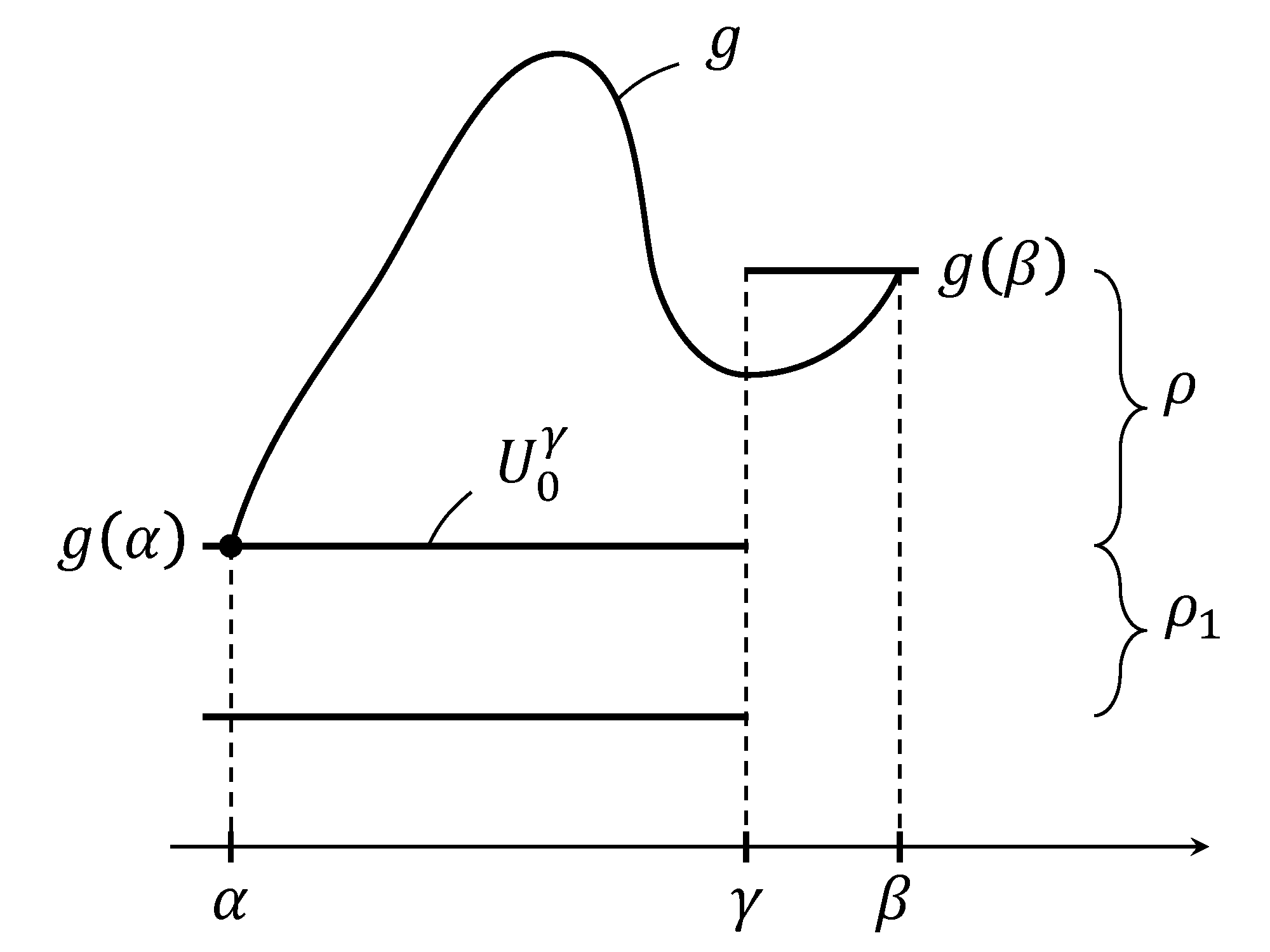
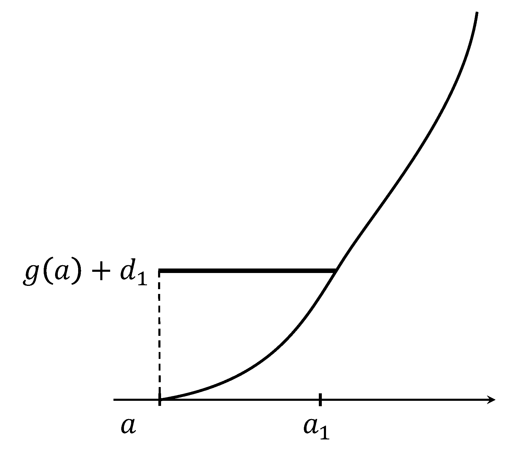
Assume that there is a jump point of with with . Then . If not, and set
For a sufficiently small , ; see Figure 1.
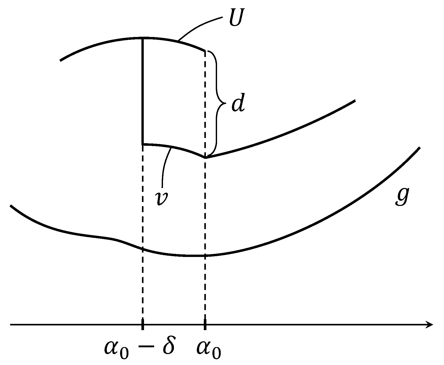
By definition, and . Thus is not a minimizer of . Similarly, if there is a jump point of with , then .
We shall prove that is continuous on provided that on . If not, there would exist a jump point of with satisfying for , , . We shall prove that such configuration does not occur. We first claim that . By symmetry, we may assume that . Since we know , we take such that
We set on . Outside , we set . If is taken close to , then on and , ; see Figure 2.
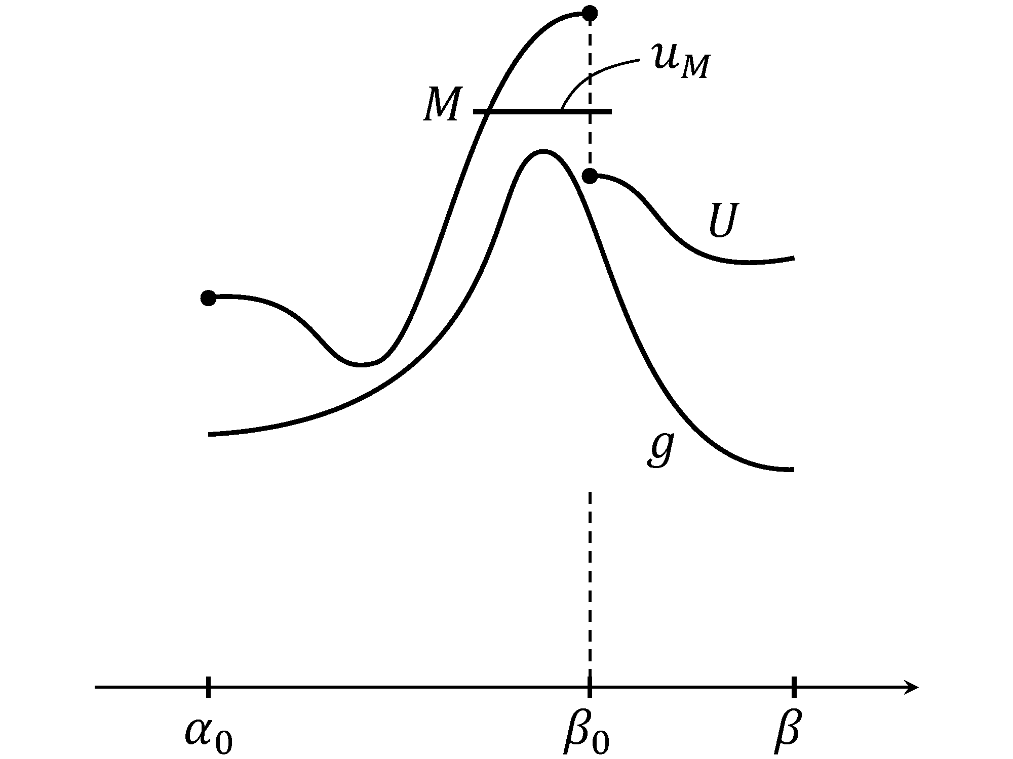
Thus and by truncation . This contradicts to the assumption that is a minimizer. Thus . However, if so, take again close to and , with . This is a contradiction so if is a jump of for , then there is no jump on provided that . In other words, is continuous and satisfies on and . We now conclude that is constant on by using a similar argument at the beginning of this proof.
Since there is a sequence of continuity point of converging to as keeping , we conclude that is a constant on . This says that is constant on . To say that this corresponds to (i), it remains to prove that . If not, , then we take
where . Here,
which is continuous and non-decreasing. Moreover,
where ; see Figure 3.
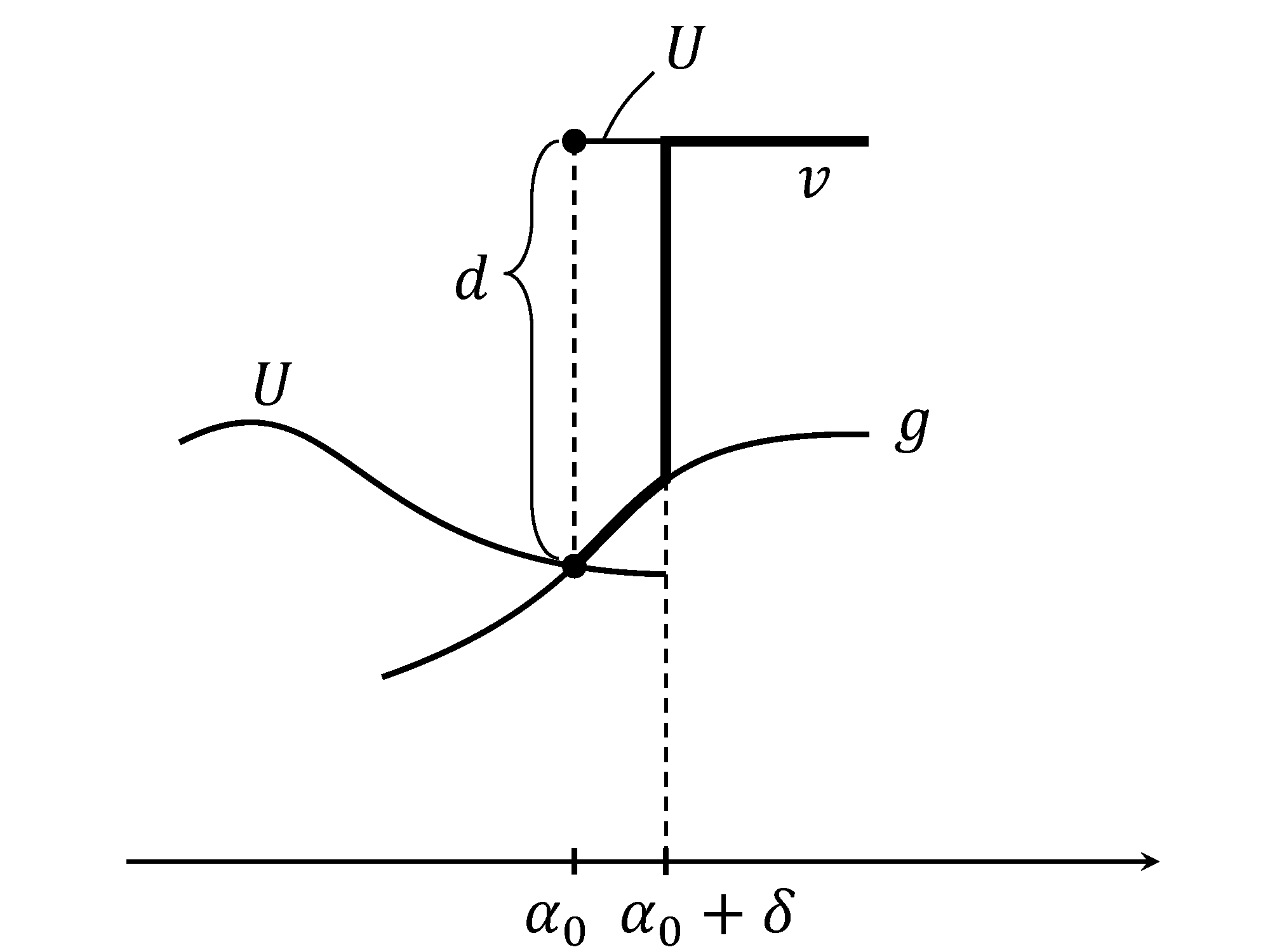
Thus
Since as , and as by (K1), we conclude that for sufficiently small , . We now obtain (i). A symmetric argument yields (ii). The proof is now complete. ∎
For and , we set
If in , we simply write
and call the coincidence set of . By Lemma 3.1, we obtain a few properties of .
Lemma 3.2.
Assume the same hypotheses of Lemma 3.1 concerning , and . Let be defined for . Then in , i.e., is continuous on the coincidence set . If with . then is piecewise constant on with at most one jump.
Proof.
By Lemma 3.1 (i) and (ii), we easily see that . Thus, is continuous on .
It remains to prove the second statement. By Lemma 3.1, the value of on is either or . Moreover, if there are more than two jumps, must take value of at some point . In other words, . This contradicts to . ∎
We conclude this section by showing that if two points with for a minimizer is too close, then must be monotone in under the assumption that satisfies (K1), (K2w) and (K3).
We first note comparison with usual total variation and .
Lemma 3.3.
Assume that satisfies (K1), (K2w) and (K3). If with is continuous at and , then
Proof.
We may assume that . By definition,
where denote the jump discontinuity of and for . We note that
where . By subadditivity (K2w), we see that
since is continuous by (K1). By (K2w), we have
for . Sending , we obtain by (K3) that
We thus observe that
The last inequality follows from the subadditivity (K2w). ∎
If we assume (K1) and (K3), we have, by (2.1),
| (3.1) |
with some positive constant depending only on . We next give our monotonicity result.
Theorem 3.4.
Assume that satisfies (K1), (K2w) and (K3), and that . Let be a minimizer of in . Let and with be in , where denotes the coincide set. If (resp. ), then is non-decreasing (non-increasing) provided that if , where is a constant (3.1).
Proof.
We first note that is continuous at by Lemma 3.2. Moreover, if there is no point of in , by Lemma 3.2, is piecewise constant with at most one jump in . Thus, is monotone.
We next consider the case that . We may assume that since the proof for the other case is symmetric. We shall prove that
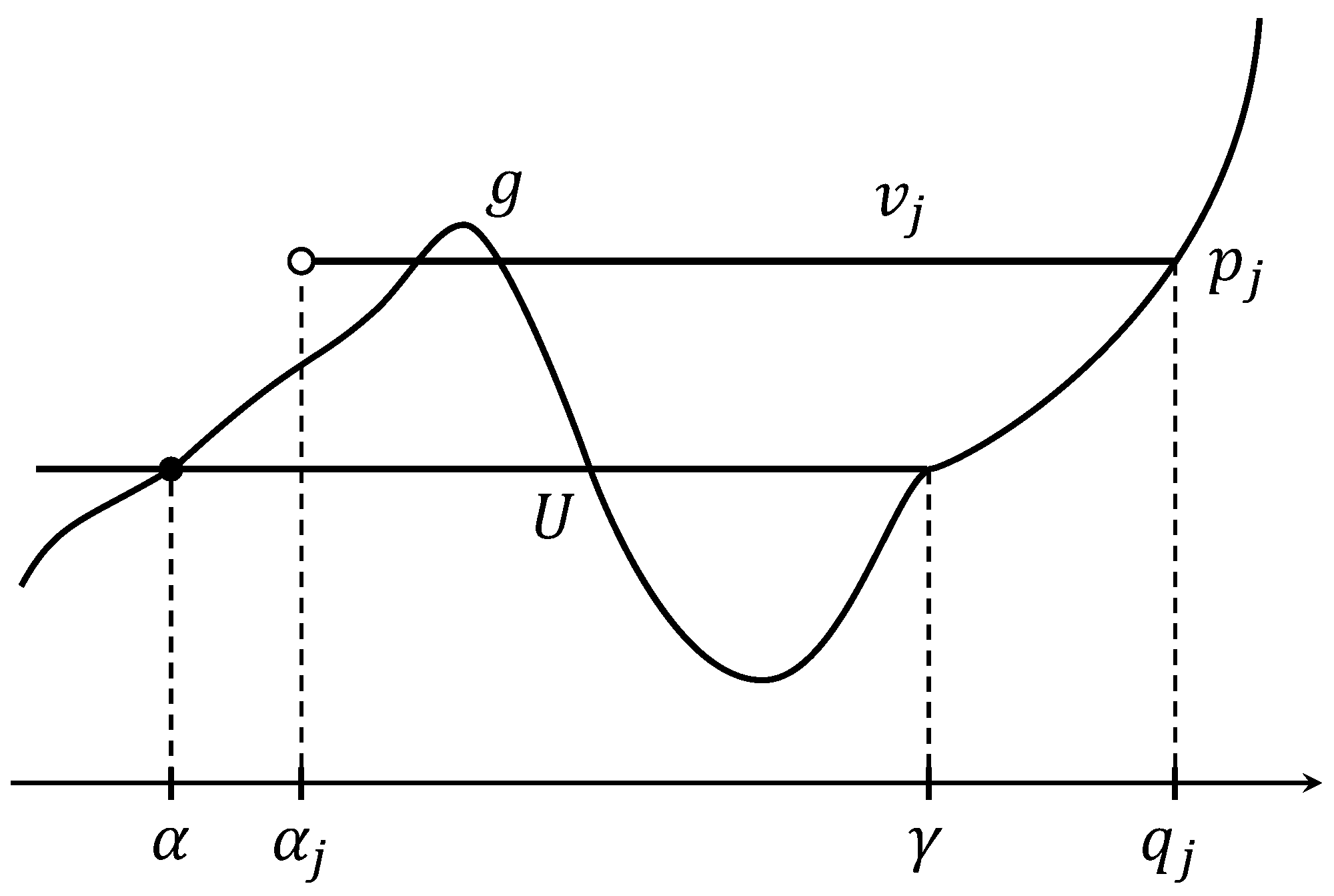
for any . Suppose that there were a point such that or . We may assume that since the proof for the other case is parallel. By Lemma 3.2, we see that there is such that
We take such that
see Figure 4.
We now define a truncated function
We shall prove that if . Since and are continuous at and ,
Since does not increase by truncation, we see
Since on , we proceed
By Lemma 3.3, we observe that
Thus by (3.1), we now obtain
We next compare the values and . By definition, we observe
The last inequality follows from the fact that the value of must be between and . We thus observe that
If satisfies , is not a minimizer provided that , i.e., . Thus, we conclude that .
So far we have proved that is non-decreasing on . By Lemma 3.2, we conclude that itself is non-decreasing in . ∎
4. Minimiziers for general one-dimensional data
In this section, we shall prove that a minimizer is piecewise linear if satisfies (K1), (K3) and (K2) instead of (K2w). In other words, we shall prove our main result.
If we assume (K2), then merging jumps decrease the value . However, may increase. We have to estimate an increase of .
4.1. Bound for an increase of fidelity
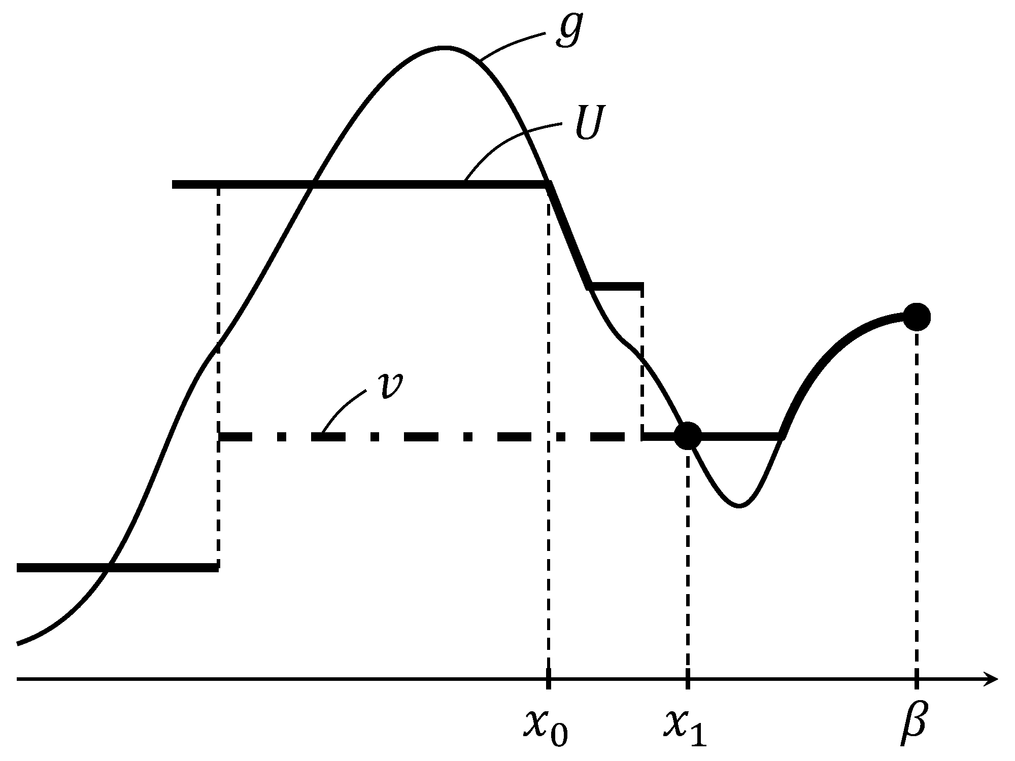
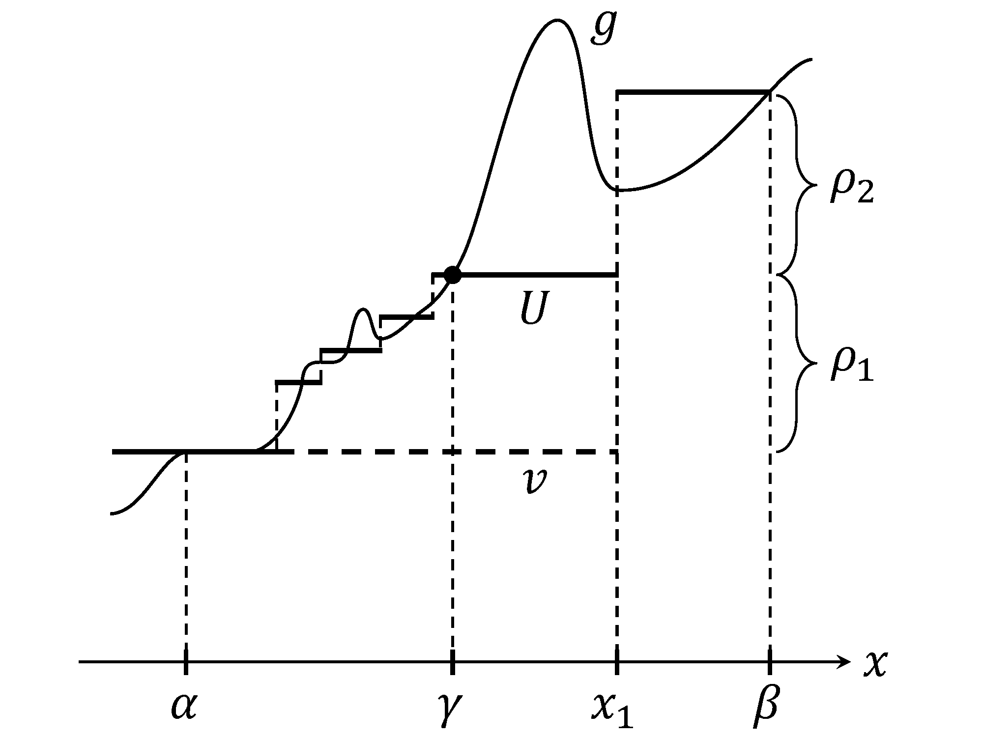
We shall estimate an increase of fidelity . We begin with a simple setting. We set
for ; see Figure 5.
The fidelity of on is still denoted by , i.e.,
for . Since we do not assume that is non-decreasing, may be very large on . Fortunately, we observe that cannot be too large on in the average if is smaller than .
Proposition 4.1.
Assume that and , with . If satisfies , then
or
Proof.
We observe that
Since , implies that
∎
We give a simple application. See Figure 5.
Lemma 4.2.
Proof.
We may assume that by adding a constant to both amd . The left-hand side equals
Since
by Proposition 4.1, we end up with . ∎
We next consider behavior of between two points of the coincidence set where is a constant.
Proposition 4.4.
Assume that satisfies (K1), (K2w) and (K3). Assume that . Let by a minimizer of . Let be and . Assume that is non-decreasing and there is such that and for . Assume that there is such that , as . Then, .
Proof.
Since is a minimizer, by definition,
By Lemma 3.3,
where . Since
implies that . In other words,
Dividing the region of integration by and , we obtain
or
Since on , the right-hand side is dominated by
Thus
Sending yields that
since by our assumption that for and is non-decreasing. The proof is now complete. ∎
We say that a closed interval is a facet of if is a maximal nontrivial closed interval such that is a constant on the interior of . Let denote its length. We are able to claim a similar statement for each facet of a minimizer .
Lemma 4.5.
Assume that satisfies (K1), (K2w) and (K3). Assume that . Let be a minimizer of . Assume that is non-decreasing. Let with be a facet of . Then
| (4.1) |
Proof.
Theorem 4.6.
Assume that satisfies (K1), (K2w) and (K3). Assume that . Let be a minimizer of . Assume that is non-decreasing. Let with . Then
when .
Proof.
If , a minimizer must be constant so the above inequality is trivially fulfilled. We may assume .
As before, we may assume so that . We proceed
On the coincidence set ,
since on . On a facet , by Lemma 4.5,
since . We now conclude that
Since with at most countably many facets , this implies that
∎
4.2. No possibility of fine structure
Our goal in this subsection is to prove our main theorem. In other words, we shall prove that a minimizer does not allow to have a “fine” structure under the assumption (K2). At the end of this subsolution, we prove our main theorem Theorem 1.1.
Lemma 4.7.
Assume that satisfies (K1), (K2) and (K3). Assume that . Let be a minimizer of . Assume that is non-decreasing. Let satisfy and . Assume that . Then
for , where is the constant in (K2).
Proof.
We set , . Since , by Lemma 3.2, has only one jump at and for , for .
From the proof of Lemma 4.7, we have a rather general estimate for defined at the beginning of Section 4.1.
Lemma 4.8.
Assume that satisfies (K1), (K2) and (K3). Assume that and . Assume that and . Let be a non-decreasing function with , which is continuous at and . Assume that where is a facet and is a coincidence set with and , . (The set for could be empty.) Assume that and . Assume further that satisfies (4.1) on each for . Assume that for . If contains an interior point of , then
with .
We are interested in the case that there are no jumps. We begin with an elementary property of .
Lemma 4.9.
Assume that satisfies (K2) and (K3). Then, .
Proof.
An iterative use of (K2) yields
for . Since as , sending yields
by (K3). The proof is now complete. ∎
Lemma 4.10.
Assume the same hypotheses of Lemma 4.7 concerning and . Let be a minimizer of . Assume that is non-decreasing and continuous on with . Then .
Proof.
Suppose that so that , there would exist at least one such that is a singleton since is continuous. By Lemma 3.1, . Moreover, there is a sequence () such that is a singleton . This is possible since the set of values where is not a singleton is at most a countable set. Since is a singleton, . Again by Lemma 3.1, . We set
By Theorem 4.6, we obtain
with .
Since for a continuous function, we see that
By Lemma 4.9, we observe that
We thus conclude that
For a sufficiently large , since . This would contradict to our assumption that is a minimizer. Thus . ∎
Theorem 4.11.
Assume that satisfies (K1), (K2) and (K3). Assume that . Let be a minimizer of . Let with . Assume that with and , where is in (3.1) and is in (K2). Then takes either or on and it has at most one jump point in .
Proof.
By Theorem 3.4, is non-decreasing in . We may assume . If there is no jump, i.e., , by Lemma 4.10, is not a minimizer so must have at least one jump point in . We take a jump point such that jump size
is maximum among all jump size of in . If , , we get the conclusion. Suppose that . We set
By Lemma 3.1, and . Since , we see . Since the jump at is a maximal jump, we apply Lemma 4.7 on to get
which would contradict the assumption . We thus conclude that . If , we consider instead of . We argue in the same way. We apply Lemma 4.7 and get a contradiction. We thus conclude that . The proof is now complete. ∎
Proof of Theorem 1.1.
By Lemma 3.1, on and is non-empty. We take an integer so that
We divide into intervals so that the length of each interval is less than and the boundaries of each interval does not contain a jump point of . (This is possible if we shift a little bit unless , or since is at most a countable set. If (resp. ), must be continuous at () since is continuous on the coincidence set by Lemma 3.2.) If is empty or singleton, then must be a constant on by Lemma 3.1. We next consider the case that has at least two points. We set
and may assume . Since , Theorem 4.11 implies that only takes two values and and has at most one jump on . By Lemma 3.1, is constant on and .
We now observe that on each , has at most one jump. We thus conclude that is a piecewise constant function with at most jumps on . ∎
4.3. Minimizers for monotone data
We shall prove that the bound for number of jumps is improved when is monotone. In other words, we shall prove Theorem 1.2.
We first observe the monotonicity of a minimizer for when is monotone.
Lemma 4.12.
Assume that satifies (K1) and that is non-decreasing. Then a minimizer of (in ) is non-decreasing.
Proof.
Let be a minimizer. We take its right continuous representation. Suppose that with some . Then a chopped function
decreases both and the fidelity term so that
see Figure 8.
Thus for , is always non-decreasing. A symmetric argument implies that is always non-decreasing for . If is not non-decreasing in , then it must jump at some with
Our competitor can be taken as
By definition, so such jump cannot occur for a minimizer. Thus is non-decreasing. ∎
Proof of Theorem 1.2.
It is not difficult to get a minimizer when is strictly increasing for , i.e.,
By Lemma 4.12, a minimizer must be non-decreasing. (In this problem, is strictly convex and lower semicontinuous in , so there exists a unique minimizer.) We note that
provided that is non-decreasing. We set , and , . To minimize , we take and such that
See Figure 9.
Then the minimizer must be
provided that . This formation of a flat part near the boundary occurs by the natural boundary condition. (In general, the minimizer has no jumps if is continuous for (cf. [CL], [GKL]).)
In the case when is monotone, we are able to prove a conclusion stronger than Proposition 4.1.
Proposition 4.13.
Assume that and , with . If satisfies , then for .
This easily follows from the next observation.
Proposition 4.14.
Assume that is non-decreasing. Then is minimized if and only if .
Proof.
A direct calculation shows that
Then
Thus, takes its only minimum at . ∎
We give a few explicit estimate of for monotone function to give an alternate proof for Theorem 1.2.
We recall . We shall simply write by if . Note that such always exists since is continuous. It is unique if is increasing. In general, it is not unique and we choose one of such . We next consider a non-decreasing piecewise constant function with two jumps. We set and and define
for with . If is minimized by moving and by Lemma 3.1, there is a point such that . Moreover, by Proposition 4.14, is minimized by taking , , where and are defined by
see Figure 10.
Again , may not be unique. We take one of them.
We shall estimate
This can be considered as a special case of Lemma 4.8 since (4.1) is automatically fulfilled by Proposition 4.13. However, the proof is clearer than that of general , we give a full proof.
Lemma 4.15.
Assume that is increasing. Let be a non-decreasing piecewise constant function with three values , , for , where . Then
Proof.
We may assume by symmetry. For , we fix and . We first observe that . We calculate
We shall estimate the second term of the right-hand side by dividing
For , we proceed
since by on so that . Since
as for , we have
We thus conclude that
This yields the desired inequality for since . ∎
We set and
Lemma 4.16.
Assume that satisfies (K1) and (K2). Assume that is non-decreasing. If and , then
for , where .
Proof.
Since is independent of the choice of , we observe that
with , . For , we set , so that . We observe that
By (K2), we observe that
for . By Lemma 4.15, we conclude that
Thus
provided that , i.e., . The proof is now complete. ∎
To prove Theorem 1.2 directly, we approximate a general function by a piecewise constant function such that is also approximated.
Lemma 4.17.
Assume that satisfies (K1), (K3) and that . For any with , there is a sequence of piecewise constant functions (with finitely many jumps) such that in and as .
Since in implies when , this lemma yields
Lemma 4.18.
Assume that satisfies (K1), (K3) and . For any , there is a sequence of piecewise constant function such that in and as .
We shall prove Lemma 4.17 by reducing the problem when is continuous, i.e., .
Lemma 4.19.
Assume that satisfies (K3) and . For any , there is a sequence of piecewise constant functions such that in and as .
Proof.
For a continuous function , agrees with usual . We extend continuously in some neighborhood if and denote it by . We mollify by a symmetric mollifier . It is well known that is in and in as . Moreover, [Giu, Proposition 1.15]. Since can be approximated (in sense) by polynomials in a bounded set, we approximate by a polynomial with its derivative in . Thus, we may assume that is a polynomial.
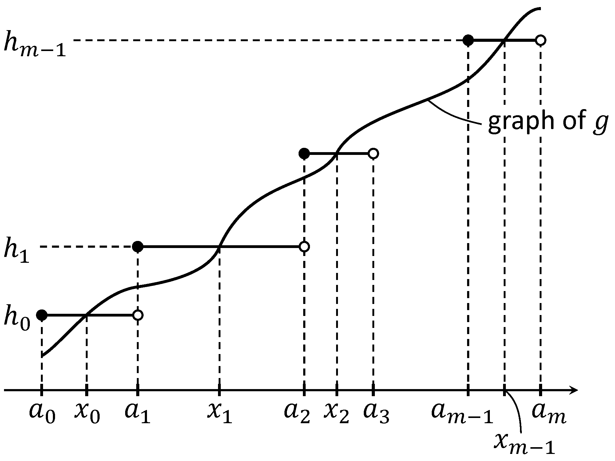
For a given , we define a piecewise constant function
We divide the interval into finitely many subintervals with such that on each such an interval is either increasing or decreasing. This is possible since is a polynomial. Let denote the total variation of in for . Then
By the assumption (K3), we see that for any there is such that for . Since is continuous, the size of jumps of is always so
where we use the same convention to . We thus observe that
Sending , we now conclude that
Since is arbitrary, the convergence as follows. By definition, in . The proof is now complete. ∎
Proof of Lemma 4.17.
Since is bounded by , for any , the set of jump discontinuities of whose jump size greater than is a finite set. For any , we take such that
We may assume that with and , . In each interval , we approximate in with continuous function . We now apply Lemma 4.19 on each interval to approximate by a piecewise constant function . Although the jump at is not exactly equal to
it converges to this value as and . We now obtain a desired sequence of piecewise constant functions. ∎
Remark 4.20.
We give a sufficient condition (Lemma 4.16) that a larger jump costs less for not only by giving a quantative estimate.
In the rest of this section, we give an alternate proof of Theorem 1.2 without using Theorem 1.1 by establishing a quantative estimate of . By approximation (Lemma 4.18), if there is a minimizer of among piecewise constant functions, this minimizer is also a minimizer of in . The existence of a minimizer among piecewise constant functions can be proved since the number of facets are restricted. We shall come back to this point at the end of this section. Unfortunately, this argument is not enough to prove Theorem 1.2 since we do not know the uniqueness of a minimizer. To show Theorem 1.2, we need a quantified version of Lemma 4.16. Let be a minimizer with one jump.
Lemma 4.21.
Assume that satisfies (K1), (K2) and (K3). Assume that is non-decreasing. Let be a constant such that . Assume that . Let is a non-decreasing function on which is continuous at and and , . Then
where and () is the set of jump discontinuities. The non-negative term
vanishes if and only if with some .
We begin with an elementary lemma on a sequence.
Lemma 4.22.
Let be an increasing sequence of natural numbers and . Let be a set of non-negative real numbers. Assume that
-
(i)
provided that .
-
(ii)
provided that .
-
(iii)
Let be the set of such that and implies . Then
Proof.
-
(i)
We may assume that . Since
and
we obtain (i).
-
(ii)
This follows from Fatou’s lemma.
-
(iii)
We divide the set of indices by and , the complement of . Since
applying the results (i), (ii) yield (iii).
∎
Proof of Lemma 4.21.
We may assume that . Let be a minimizer of on . Its existence is proved in Section 2. By Lemma 4.12, is non-decreasing. Moreover, by Lemma 3.2, is a piecewise constant outside the set
and each facet contains a point such that and is continuous at . We set
By definition, and . By Lemma 4.12 and Lemma 3.2, and is continuous at and . We approximate on by a piecewise constant non-decreasing function with facets by Lemma 4.19. Since is continuous at and , we may assume that for close to and for close to . We denote jumps by with and set with convention that , . We set
which denotes the jump at each . We fix and minimize on . In other words, we minimize by moving ’s. Let be its minimizer. By Proposition 4.14, facets of consist of
with , ; see Figure 11 with , .
By this choice,
We shall estimate from below as in Lemma 4.16. For , let be a piecewise constant function on with one jump at the point such that
We set
We note that . Since , we argue as in Lemma 4.16 and observe that
From now on, we write jumps of by instead of . Our estimate for yields
Since in and , we observe, by changing numbering of in if necessary, that as for such that corresponds to jumps at of and for other ’s. The convergence of prevents that two jumps with positive length merges at the limit unless one of them tends to zero. Let be the set such that . We now apply Lemma 4.22 to conclude that
where . Since
the quantity
if and only if and , i.e., is a singleton, i.e., with some and . ∎
We conclude this subsection by proving Theorem 1.2 based on the quantative estimate.
Alternate proof of Theorem 1.2.
Again, we may assume that is not a constant. By Lemma 4.12, a minimizer is non-decreasing. By Lemma 3.2, at the place where , the function is continuous. Let be the set of such that
are not a singleton. We set
Since is continuous, is not empty by Lemma 3.1.
If we prove that is a discrete set so that it is a finite set. Then, by Lemma 3.1, is a piecewise constant function. We shall prove that is a discrete set. By definition, if for , then . Suppose that were not discrete, then for any small , there would exist with such that the interval would contain infinitely many element of . Since minimizes on with , , applying Lemma 4.21 to , to conclude that must have at most one jump provided that . This yields a contradiction so we conclude that is discrete and is a non-decreasing piecewise constant function. The number of jumps can be estimated since the distance of two points in is at most . ∎
4.4. Application of approximation lemma
We shall prove Theorem 1.3. We approximate by such that in as and
for all . Let with . By Lemma 4.17, there is a sequence of piecewise constant functions such that with in as . We thus observe that is a “recovery” sequence in the sense that . Let be a minimizer of . By Theorem 1.1, the number of jump is bounded by
with . By compactness of a bounded set in a finite dimensional space, has a convergent subsequence, i.e., with some in (and also with respect to weak* topology of ). Moreover, the limit is still a piecewise constant function with at most jumps. By lower semicontinuity of (Proposition 2.4), we see that
We thus conclude that is a desired minimizer of since is an arbitrary element.
5. A sufficient condition for (K2)
We give a sufficient condition for (K2) if is derived as a limit of the Kobayashi-Warren-Carter energy, i.e., is of the form (1.7).
We first consider a kind of Fenchel dual of a function . We set
| (5.1) |
for a real-valued function on . If we use the Fenchel dual, it can be written as
where for and for . We assume
-
(f1)
;
-
(f2)
takes the only minimum at . In other words, for all and if and only if ;
-
(f3)
for .
Lemma 5.1.
Assume (f2). Then for and . Assume further (f2) and (f3). Then for all and there is for such that and is strictly increasing in . Moreover, is strictly increasing and as . Furthermore, it satisfies (K2) with if satisfies
| (5.2) |
Here we define
Proof.
The positivity for for and is clear by the definition (5.1). Also, the existence in of a minimizer easily follows by (f1) and (f2). Although may not be unique, as well as monotonicity of is guaranteed by (f3). The bound is rather clear.
Lemma 5.2.
Assume that (f1), (f2) and (f3). Then . In other words, satisfies (K3) with .
Proof.
Remark 5.3.
- (i)
- (ii)
-
(iii)
We may take other element of a preimage of of but as a sufficient condition the present choice is the weakest assumption.
We come back to (1.7). In other words,
We assume that
-
(F1)
and takes the only minimum at .
If we set , the property (F1) implies (f1), (f2) and (f3). Since (5.2) is property near , (5.2) for and are equivalent. We thus obtain an sufficient condition so that in (1.7) satisfies (K1), (K2) and (K3)
Proposition 5.4.
Proof.
We conclude this section by examining the property (5.4). The left-hand side is equivalent to saying that
where . We set
The condition (5.4) is now equivalent to
| (5.5) |
where . To simplify the argument, we further assume that
-
(F2)
in so that the inverse function in is uniquely determined.
If we assume (F1) and (F2), by changing the variable of integration , we have
The condition (5.5) is fulfilled if
or equivalently
We thus obtain a simple sufficient condition.
Theorem 5.5.
Assume that (F1) and (F2). Then in (1.7) satisfies (K1), (K2), (K3) provided that
Acknowledgements
The work of the first author was partly supported by JSPS KAKENHI Grant Numbers JP19H00639, JP20K20342, JP24K00531 and JP24H00183 and by Arithmer Inc., Daikin Industries, Ltd. and Ebara Corporation through collaborative grants. The work of the third author was partly supported by JSPS KAKENHI Grant Number JP20K20342. The work of the fifth author was partly supported by JSPS KAKENHI Grant Numbers JP22K03425, JP22K18677, 23H00086.
References
- [AFP] L. Ambrosio, N. Fusco and D. Pallara, Functions of bounded variation and free discontinuity problems. Oxford Mathematical Monographs, Clarendon Press, Oxford University Press, New York, 2000.
- [AT] L. Ambrosio and V. M. Tortorelli, Approximation of functionals depending on jumps by elliptic functionals via -convergence. Comm. Pure Appl. Math. 43 (1990), no. 8, 999–1036.
- [AT2] L. Ambrosio and V. M. Tortorelli, On the approximation of free discontinuity problems. Boll. Un. Mat. Ital. B (7) 6 (1992), no. 1, 105–123.
- [BB] G. Bouchitté and G. Buttazzo, New lower semicontinuity results for nonconvex functionals defined on measures. Nonlinear Anal. 15 (1990), no. 7, 679–692.
- [CCN] V. Caselles, A. Chambolle and M. Novaga, The discontinuity set of solutions of the TV denoising problem and some extensions. Multiscale Model. Simul. 6 (2007), no. 3, 879–894.
- [CL] A. Chambolle and M. Łasica Inclusion and estimates for the jumps of minimizers in variational denoising. arXiv: 2312.01900 (2023).
- [DN] G. Del Nin, Rectifiability of the jump set of locally integrable functions. Ann. Sc. Norm. Super. Pisa Cl. Sci. (5) 22 (2021), no. 3, 1233–1240.
- [ELM] Y. Epshteyn, C. Liu and M. Mizuno, Motion of grain boundaries with dynamic lattice misorientations and with triple junctions drag. SIAM J. Math. Anal. 53 (2021), no. 3, 3072–3097.
- [FL] I. Fonseca and P. Liu, The weighted Ambrosio-Tortorelli approximation scheme. SIAM J. Math. Anal. 49 (2017), no. 6, 4491–4520.
- [GaFSp] A. Garroni, M. Fortuna and E. Spadaro, On the Read-Shockley energy for grain boundaries in poly-crystals. arXiv: 2306.07742 (2023).
- [GKL] Y. Giga, H. Kuroda and M. Łasica, A few topics on total variation flows, preprint.
- [GOSU] Y. Giga, J. Okamoto, K. Sakakibara and M. Uesaka, On a singular limit of the Kobayashi-Warren-Carter energy. Indiana Univ. Math. J., accepted for publication.
- [GOU] Y. Giga, J. Okamoto and M. Uesaka, A finer singular limit of a single-well Modica-Mortola functional and its applications to the Kobayashi-Warren-Carter energy. Adv. Calc. Var. 16 (2023), no. 1, 163–182.
- [GU] Y. Giga and M. Uesaka, On a diffuse intefacial energy with a phase structure and its singular limit (in Japanese). Bulletin of the Japan Society for Industrial and Applied Mathematics (Ōyō Sūri) 32 (2022), 186–197.
- [GCL] E. De Giorgi, M. Carriero and A. Leaci, Existence theorem for a minimum problem with free discontinuity set. Arch. Rational Mech. Anal. 108 (1989), no. 3, 195–218.
- [Giu] E. Giusti, Minimal surfaces and functions of bounded variation. Monogr. Math., 80, Birkhäuser Verlag, Basel, 1984, xii+240 pp.
- [KWC1] R. Kobayashi, J. A. Warren and W. C. Carter, A continuum model of grain boundaries. Phys. D 140 (2000), no. 1–2, 141–150.
- [KWC2] R. Kobayashi, J. A. Warren and W. C. Carter, Grain boundary model and singular diffusivity. GAKUTO Internat. Ser. Math. Sci. Appl. 14 Gakkōtosho Co., Ltd., Tokyo, 2000, 283–294.
- [LL] G. Lauteri and S. Luckhaus, An energy estimate for dislocation configurations and the emergence of Cosserat-type structures in metal plasticity. arXiv: 1608.06155 (2017).
- [ROF] L. Rudin, S. Osher and E. Fatemi, Nonlinear total variation based noise removal algorithms. Experimental mathematics: computational issues in nonlinear science (Los Alamos, NM, 1991), Phys. D 60 (1992), no. 1–4, 259–268.
- [WKC] J. A. Warren, R. Kobayashi and W. C. Carter, Modeling grain boundaries using a phase-field technique. J. Crystal Growth 211 (2000), no. 1–4, 18–20.