Physics-aware Reduced-order Modeling of Transonic Flow via $\beta$-Variational Autoencoder

The AE model is a widely used deep learning-based DR technique. The main objective of the AE is to output exactly what is inputted. Its structure consists of two parts: an encoder and a decoder. The input of the AE, x, is entered into the encoder for the compression and exits as LVs, z. Then, z enters the decoder and exits as reconstructed data $\tilde{\textbf{x}}$. The encoder and decoder consist of a multi-layer perceptron (MLP), which makes it possible to model nonlinearity in the reduction and reconstruction processes. Because the objective of training the AE model is to reconstruct $\tilde{\textbf{x}}$ similar to the original data x, the loss function is defined by Eq. 1, where $N$ denotes the number of data samples. Although its loss function is defined by the mean square error (MSE) in this study, any other error metrics, such as the binary cross entropy between x and $\tilde{\textbf{x}}$, can be used depending on the properties of the data. Note that the adopted MSE is the mean operation over sample-wise, and the summation over element-wise (pixel-wise) directions.

$$\ \mathcal{L}_{AE}=\frac{1}{N}\sum\limits_{i=1}^{N}{(\textbf{x}_{i}-\tilde{\textbf{x}}_{i})^{2}},$$

(1)

However, this AE model has a obvious limitation: there is no training algorithm for guaranteeing a regularized latent space. Herein, the expression “regularized latent space” means that the latent space is trained to be smooth and continuous; thus, when inputs $\textbf{x}_{1}$ and $\textbf{x}_{2}$ are similar (or close), their corresponding mapped latent space, $\textbf{z}_{1}$ and $\textbf{z}_{2}$, should also be similar [28]. In AE model, as the original input x becomes condensed layer-by-layer through the encoder, its representation becomes increasingly abstract [29]. Therefore, the output of the encoder z is not guaranteed to be regularized in the training procedure of the AE. This explains why the decoder part of the AE model cannot be used as a generative model: the trained latent space is irregular and therefore its correlation with the reconstructed data is abstract.

Many studies have focused on the limitations of this unregularized latent space trained by an AE and have alternatively applied VAE in their framework. The structure of the VAE is similar to that of the AE. One major difference is that VAE stochastically extracts the latent space z via random sampling, whereas the AE model obtains its latent space deterministically.

The mathematical formulae for the VAE model are presented below (for further details, please refer to these references [24, 30]). We consider reducing the original dataset $\textbf{X}=\left\{\textbf{x}_{i}\right\}_{N}^{i=1}$ (assumed to be independently and identically distributed) to the latent space z using the VAE model. In the inference of z from X, variational inference is adopted due to the intractability of the posterior $p_{\mathbf{\theta}}(\textbf{z}|\textbf{x})$, where $\mathbf{\theta}$ is a parameter of the VAE model (to be more specific, it is intractable owing to the likelihood of $p_{\mathbf{\theta}}(\textbf{z})$). Therefore, instead of the intractable posterior $p_{\mathbf{\theta}}(\textbf{z}|\textbf{x})$, the VAE is trained to obtain its substitute, $q_{\mathbf{\phi}}(\textbf{z}|\textbf{x})$ ($\mathbf{\phi}$ is a variational parameter). Then, the log-likelihood of $p_{\mathbf{\theta}}(\textbf{x})$ can be expressed as:

$$\ \log(p_{\mathbf{\theta}}(\textbf{x}))=\int{\log{(\frac{p_{\mathbf{\theta}}(\textbf{x},\textbf{z})}{q_{\mathbf{\phi}}(\textbf{z}|\textbf{x})})}q_{\mathbf{\phi}}(\textbf{z}|\textbf{x})d\textbf{z}}+\int{\log{(\frac{q_{\mathbf{\phi}}(\textbf{z}|\textbf{x})}{p_{\mathbf{\theta}}(\textbf{z}|\textbf{x})})}q_{\mathbf{\phi}}(\textbf{z}|\textbf{x})d\textbf{z}},$$

(2)

where the second term on the right-hand side (RHS) is the KL-divergence of $q_{\mathbf{\phi}}(\textbf{z}|\textbf{x})$ from $p_{\mathbf{\theta}}(\textbf{z}|\textbf{x})$, $KL(q_{\mathbf{\phi}}(\textbf{z}|\textbf{x})||p_{\mathbf{\theta}}(\textbf{z}|\textbf{x}))$, which is always non-negative according to its definition (KL-divergence is a measurement of the statistical distance between two probability distributions). Therefore, the first term on the RHS becomes the lower bound of the log-likelihood and the problem of maximizing the log-likelihood becomes the problem of maximizing the lower bound. This lower bound can be expressed as:

$$\ \int{\log{(\frac{p_{\mathbf{\theta}}(\textbf{x},\textbf{z})}{q_{\mathbf{\phi}}(\textbf{z}|\textbf{x})})}q_{\mathbf{\phi}}(\textbf{z}|\textbf{x})d\textbf{z}}=\mathbb{E}_{q_{\mathbf{\phi}}(\textbf{z}|\textbf{x})}{[\log{p_{\mathbf{\theta}}(\textbf{x}|\textbf{z})}]}-\int{\log{(\frac{q_{\mathbf{\phi}}(\textbf{z}|\textbf{x})}{p_{\mathbf{\theta}}(\textbf{z})})}q_{\mathbf{\phi}}(\textbf{z}|\textbf{x})d\textbf{z}},$$

(3)

where the first and second terms on the RHS are the reconstruction error and KL-divergence of $q_{\mathbf{\phi}}(\textbf{z}|\textbf{x})$ from $p_{\mathbf{\theta}}(\textbf{z})$, respectively. However, owing to the existence of $q_{\mathbf{\phi}}(\textbf{z}|\textbf{x})$ in the reconstruction error, the back-propagation process cannot be performed, and calculating the gradient of the reconstruction error with respect to $\mathbf{\phi}$ is problematic due to the posterior $q_{\mathbf{\phi}}(\textbf{z}|\textbf{x})$. Therefore, a “reparameterization trick” is adopted, which allows for back-propagation during the sampling process. The concept behind this trick is to sample z from the auxiliary noise variable $\epsilon\sim N(0,1^{2})$: this random sampling makes the latent space in the VAE stochastically determined. To be more specific, the $\rm k^{th}$ LV ($z_{k}$) is assumed to follow the distribution below:

$$\ z_{k}=\mu_{k}+\sigma_{k}\odot\epsilon.$$

(4)

where $\odot$ denotes Hadamard product (element-wise product). Accordingly, the KL-divergence, the second term on the RHS in Eq. 3 can be rewritten as below when the posterior $q_{\mathbf{\phi}}(\textbf{z}|\textbf{x})$ and prior $p_{\mathbf{\theta}}(\textbf{z})$ are assumed to follow the Gaussian distribution $N(\mathbf{\mu},\mathbf{\sigma}^{2})$ and $N(0,\textbf{I}^{2})$, respectively.

$$\ KL(q_{\mathbf{\phi}}(\textbf{z}|\textbf{x})||p_{\mathbf{\theta}}(\textbf{z}))=\frac{1}{2}\sum\limits_{k=1}^{d}{(\sigma_{k}^{2}+\mu_{k}^{2}-(\log(\sigma_{k}^{2})+1))},$$

(5)

where $\mu_{k}$ and $\sigma_{k}$ represent the mean and standard deviation used during the reparameterization of $z_{k}$, and $d$ denotes the dimension of the latent space. Herein, as the posterior approximation $q_{\mathbf{\phi}}(\textbf{z}|\textbf{x})$ approaches the prior $p_{\mathbf{\theta}}(\textbf{z})$, the KL-divergence decreases. Finally, the loss function of VAE model can be formulated as in Eq. 6, which consists of the reconstruction error (MSE term) and regularizer (KL-divergence term). Since the KL-divergence term serves to regularize the latent space to be trained, it is also called regularization loss. It induces a sparser latent space [24, 31, 23, 32] just as the L1 regularization term makes the model sparse in the Lasso regression [33].

$$\ \begin{aligned} \mathcal{L}_{VAE}&=\mathcal{L}_{AE}+KL(q_{\mathbf{\phi}}(\textbf{z}|\textbf{x})||p_{\mathbf{\theta}}(\textbf{z}))\\ &=\frac{1}{N}\sum\limits_{i=1}^{N}{(\textbf{x}_{i}-\tilde{\textbf{x}}_{i})^{2}}+\frac{1}{2}\sum\limits_{k=1}^{d}{(\sigma_{k}^{2}+\mu_{k}^{2}-(\log(\sigma_{k}^{2})+1))}.\end{aligned}$$

(6)

Higgins et al. [23] focused on the trade-off relationship between the reconstruction error and KL-divergence in the loss function of the VAE. As the reconstruction accuracy increases, the degree of regularization (or information capacity) in the latent space decreases. To tune the balance between these two performances, Higgins et al. [23] proposed the $\beta$-VAE, which can control the relative importance of the KL-divergence term using the adjustable hyperparameter $\beta$. It is a simple modification of the VAE: they have exactly the same structures but slightly different loss functions. The loss function of the $\beta$-VAE is as follows:

$$\ \mathcal{L}_{\beta{\text{-}}VAE}=\frac{1}{N}\sum\limits_{i=1}^{N}{(\textbf{x}_{i}-\tilde{\textbf{x}}_{i})^{2}}+\beta KL(q_{\mathbf{\phi}}(\textbf{z}|\textbf{x})||p_{\mathbf{\theta}}(\textbf{z})).$$

(7)

The only difference in the loss functions between the VAE and $\beta$-VAE is whether the KL-divergence term is weighted by hyperparameter $\beta$. By introducing this hyperparameter, Higgins et al. [23] achieved quantitative and qualitative improvements in the disentanglement within the latent representations over the traditional VAE model. Finally, they concluded that owing to the disentangling performance of $\beta$-VAE, the interpretable representations of the independent generating factors of the given dataset can be discovered automatically. In this paper, the terminologies “disentanglement”, “interpretability”, “independence”, and “orthogonality” are used interchangeably to refer to the following property of LVs: single LV stands for a single representation feature without the intervention of other LVs. However, what makes $\beta$-VAE special is not only in its disentangling performance. The regularization loss (KL-divergence) is known to have sparsification effect to encourage the most efficient representation learning [23]. Burda et al. and Sønderby et al. practically confirmed this effect in that some LVs become inactive during the training process of VAE [25, 34]. In particular, Burda et al. confirmed that inactive LVs have a negligible effect on the reconstruction. This finding indicates that VAE trains its LVs in an efficient manner by selectively activating LVs to contain the only necessary information. Since $\beta$-VAE model also has regularization term in the loss function and even weighted by the hyperparameter $\beta$, it can be easily inferred that the sparsification effect in the $\beta$-VAE model will become more dominant as $\beta$ increases. Taking these two outstanding advantages of $\beta$-VAE, disentangled and information-intensive latent space, a novel ROM framework is proposed in the next section.

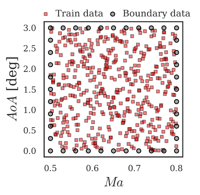
A 2D transonic flow problem, the benchmark case that is widely used in previous ROM studies [9, 10, 8, 17], is adopted for validation of the proposed physics-aware ROM. The transonic flow field is generated by the KFLOW finite-volume-based CFD solver [35, 36]. Specifically, the Reynolds-averaged Navier-Stokes equation is solved coupled with the Spalart-Allmaras turbulence model. RAE 2822 airfoil is selected as the baseline geometry, and a structured O-grid with a shape of $512\times 256$ (wall-tangential direction $\times$ wall-normal direction) is generated; the corresponding grid is shown in Fig. 3. The Reynolds number is fixed at $6.5\times 10^{6}$, and two physical parameters are chosen: $Ma$ and $AoA$. The design space of each variable is set to [0.5, 0.8] and [$0^{\circ}$, $3^{\circ}$], respectively. Latin hypercube design is used to generate 500 sample points in 2D parameter space. A flow analysis of these samples is then conducted and the resultant velocity and pressure fields are normalized by their far-field conditions. As the variations of flow properties far from the airfoil are negligible, only the inner half of the entire grid with respect to the normal direction from the airfoil is used so that the resultant grid becomes $512\times 128$. Consequently, a total dataset with a shape of $500\times 3\times 512\times 128$ (dataset size $\times$ flow field components $\times$ wall-tangential direction grids $\times$ wall-normal direction grids) is obtained, where the flow-field components are the x-velocity, y-velocity, and pressure. Finally, the dataset size of 500 is split into a ratio of 9:1 so that the size of the training dataset is 450, and that of the test dataset is 50.

In this study, all the models mentioned in Sec. 2, AE, VAE, and $\beta$-VAE, are trained to investigate their differences in terms of ROM for transonic flow. In particular, several $\beta$-VAE models are trained ($\beta\in[10,20,30,40,50,100,150,200,500,750,1000,2000,3000,4000]$) to investigate the effects of the $\beta$ value (technically speaking, $\beta$-VAE can be regarded as the VAE when $\beta$ has a value of 1). For all models, the dimension of the latent space should be determined blindly before the model training. The selected dimensions should be sufficient for encoding the training data generated from the 2D parameter domain ($Ma$ and $AoA$). In this regard, we adopted the approach suggested by Wang et al. which infers the latent dimension of $\beta$-VAE considering the accuracy of the POD with the same dimension [17] (their assumption was that POD requires much more dimensions than $\beta$-VAE for the equivalent reconstruction accuracy, which was also proved in their paper). Finally, dimension of the latent space is determined to be 16 since it conserves 99.18$\%$ in terms of energy contents of POD, which is judged to be sufficient.

An appropriate encoder/decoder structure should be selected to effectively compress/reconstruct the data, from dimensions of 3$\times$512$\times$128 to 16 and vice versa. To determine suitable structures, hyperparameter tuning based on a grid search was conducted. Finally, it was confirmed that the MSE reconstruction error, which represents the overall accuracy of the trained model, does not strongly depend on whether batch normalization, max-pooling, and up-sampling are applied. However, their application significantly affects the smoothness of the reconstructed flow field (it can be inferred that this is due to the effects of batch normalization and max-pooling that prevent overfitting, and the interpolation effect of up-sampling). If an artificial discontinuity (rather than a discontinuity that reflects a physical phenomenon, such as a shock wave) is observed in the reconstructed flow field, the flow field cannot be considered realistic. Finally, the architectures of the selected models, which are considered to be sufficient in terms of MSE error and the smoothness of the reconstructed flow field, are shown in Tables 1 and 2 and Fig. 4. The only difference between the structure of the AE and VAE/$\beta$-VAE is the bottleneck, and the structures of the VAE and $\beta$-VAE are exactly the same.

The Adam optimizer is adopted to train selected models. The initial learning rate is set to $10^{-3}$, and it decays at a rate of 0.1 every 1000 epochs. The maximum epoch should be selected carefully because a model that does not fully converge can make significantly different predictions from a converged model [37]. The maximum number of epochs is set to 3000 since it is verified to guarantee sufficient convergence in terms of the loss function. A mini-batch size of 50 is selected so that nine iterations are performed per epoch (as the size of the training dataset is 450). Using a Tesla P100-PCIE-16GB GPU with Pytorch deep learning library [38], the average training time for each model is calculated to be approximately 3 h.

First, the resultant loss functions of the trained models are shown in Fig. 5. More specifically, the loss function is decomposed into the MSE and KL-divergence (as in Eq. 7) to confirm their trade-off relationship. The MSE and KL-divergence of the VAE/$\beta$-VAE models are indicated by blue and red symbols, respectively. The $\beta$ and KL-divergence values cannot be defined in the AE model; therefore, only its MSE loss is indicated separately by a dashed line. Herein, a clear trade-off relationship between MSE and KL-divergence can be confirmed, as mentioned by Higgins et al. [23]. As $\beta$ increases, KL-divergence decreases, while MSE increases. This is consistent with the concept of the $\beta$-VAE, which suppresses KL-divergence by increasing $\beta$. In particular, when $\beta>1000$, the MSE increases significantly so that an accurate reconstruction of the flow field is no longer possible.

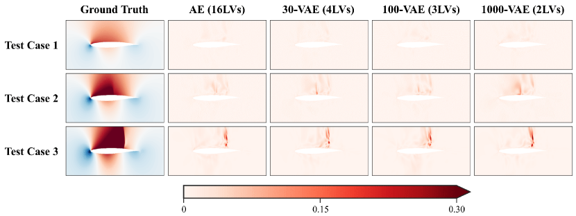
Second, the reconstructed pressure flow fields of the three test cases (which are not used during the training process) are shown in Fig. 6 to compare the trained models more intuitively and visually. The selected test cases are as follows: test case 1 is in the absence of a shock wave ($Ma=0.61$ and $AoA=2.12^{\circ}$), test case 2 is in the presence of a weak shock wave ($Ma=0.72$ and $AoA=1.68^{\circ}$), and test case 3 is in the presence of a strong shock wave ($Ma=0.78$ and $AoA=1.57^{\circ}$). Five models are compared, including the AE, VAE, 30-VAE ($\beta$-VAE with $\beta=30$), 100-VAE ($\beta=100$), and 1000-VAE ($\beta=1000$). In Fig. 6, it can be confirmed that the reconstructed pressure contours for all three cases and all models do not exhibit any significant difference, indicating all models have been trained to reconstruct the accurate flow fields.

This section is to confirm whether LVs of $\beta$-VAE are actually trained to be disentangled from each other so that they are interpretable. In Fig. 7, the absolute values of the components in the Pearson correlation matrix are shown from AE to 1000-VAE. Since there is no algorithm in AE model to promote the independence of LVs, it has the largest values. However, in $\beta$-VAEs, their values decrease as $\beta$ increases, which indicates that the LVs gradually become independent of each other. These results practically prove that the KL-divergence actually encourages the independence of each LV. To measure the degree of correlation within the entire set of LVs, Eivazi et al. computed the determinant of the correlation matrix (when the determinant is 0/1, it indicates that these variables are completely correlated/uncorrelated) [27]. However, given the fact that the KL-divergence term leads to a sparser latent space, which will be discussed in detail in Sec. 5.3, examining the determinant of the whole matrix size of $16\times 16$ is contradictory. Therefore, the independence of various LV combinations is further analyzed. First, all possible combinations of two to seven LVs are obtained. Then, the determinants of these combinations are calculated and their statistics are summarized in Fig. 8. For any number of LVs used in a combination, the $\beta$-VAE models have significantly higher determinants than the AE and VAE models. In summary, the results presented in Fig. 7 and 8 consistently show that the $\beta$-VAE successfully learns uncorrelated LVs compared to AE and VAE models, owing to the KL-divergence, which forces the LVs to be independent.

It was verified in Sec. 5.2 that the LVs in $\beta$-VAE are trained to contain disentangled information. In this section, we tried to rank such disentangled LVs according to their information intensity using KL-divergence. Fig. 9 shows the KL-divergence of each LV in AE/VAE/$\beta$-VAE. It can be confirmed that both the AE and VAE models do not have any inactive LVs. On the contrary, notable trends are observed in 30-VAE, 100-VAE, and 1000-VAE models: each model has only four (LV index 6, 8, 11, and 15), three (index 8, 11, and 15), and two (index 8 and 11) activated LVs. These results are consistent with those of Eivazi et al. in that the number of activated LVs decreases as beta increases in the $\beta$-VAE model [27]. In fact, a similar approach was applied by Sønderby et al., who judged whether the LV is activated via the KL-divergence [34]. However, the relationship between the activeness of the LV and KL-divergence was not described clearly. Therefore, we also attempt to clarify it: further investigations are conducted to check whether the LV judged to be more active in terms of the KL-divergence actually has a greater effect on the reconstructed flow field. Sobol sensitivity analysis is utilized for this analysis [39, 40]. A total 18,432 latent vectors are sampled using the Saltelli sampler in the range of $[\hat{\mu}_{k}-2\hat{\sigma}_{k},\hat{\mu}_{k}+2\hat{\sigma}_{k}]$, where $\hat{\mu}_{k}$ and $\hat{\sigma}_{k}$ each represents estimated mean and standard deviation of $\rm k^{th}$ LV with respect to the training dataset. The corresponding reconstructed flow fields are obtained through the decoder parts of the AE/VAE/$\beta$-VAE models. Since Sobol analysis should be conducted on the scalar output, a set of 3$\times$512$\times$128 pixels of the flow fields is converted to a scalar value. The sum of all pixel components is used in this study, but any scalar value representing the main characteristics of the flow field can be used. Fig. 9 shows the calculated first-order Sobol indices. It can be confirmed that the higher the KL-divergence, the larger the value of the Sobol indices in the VAE/$\beta$-VAE models (because KL-divergence has nothing to do with the algorithm of the AE model, it does not exhibit a clear trend with the Sobol indices).

Additionally, since the standard deviation represents the dispersion of the variable, which can be regarded as its activeness, $\hat{\sigma}_{k}$ values are also investigated. When $\hat{\sigma}_{k}$ is low for a specific LV, it can be understood that the corresponding LV remains inactive (or less dispersed) in the latent space during training: a situation where the value of the LV does not change even if the input data changes. In Fig. 10, it can be confirmed again that both AE and VAE models do not have any inactive LVs in that all $\hat{\sigma}_{k}$ values are larger than 0.5. However, the most interesting point is that compared to Fig. 9, LVs with high KL-divergence also have high $\hat{\sigma}_{k}$ in 30-VAE, 100-VAE, and 1000-VAE models: the LV indices of the activated LVs in terms of KL-divergence exactly match those of $\hat{\sigma}_{k}$. To sum up, we suggest the use of KL-divergence as a criterion for ranking the activeness (information intensity) of LVs for the two reasons. First, it is a regularization loss, which is the direct cause of the information discrepancies between LVs. Second, it does not require any cumbersome post-processing. The justification of this decision-making process is successfully performed through intuitive but quantitative investigations by comparing its ranking with the Sobol indices (Fig. 9) and estimated standard deviations from the training dataset (Fig. 10).

So far, using proposed KL-divergence criterion, the inactiveness within the latent space has been investigated in a quantitative manner, but it does not provide straightforward information on what these activated/inactivated variables actually contain. Accordingly, each LV is visualized via a traversal of itself, which is the most widely adopted approach for this purpose [30, 23]: it shows the traversal of a single LV while other LVs remain fixed so that one can visually understand the features of a specific LV without the intervention of other variables. In this study, a latent traversal plot is applied to identify the physical features of the flow field contained in each LV. Fig. 11 shows the pressure flow fields for two extreme LVs: one is the most dominant LV, which is ranked first by KL-divergence, and the other is the most trivial LV, which is ranked last. In AE, the pressure field changes abruptly as the most dominant LV changes; when the most trivial LV changes, the field changes gradually, but not as significant as that of the most dominant LV. Since the sparsification effect does not occur in AE due to the absence of KL-divergence term in the loss function, all the variables are activated and therefore contain uninterpretable (or entangled) physical features. However, in VAE and 1000-VAE models, the most trivial LVs cause indistinguishable variations in the flow fields. This is because the KL-divergence forces inactiveness in the latent space, so only necessary LVs become activated to contain meaningful physical features: it can be regarded as a virtue of $\beta$-VAE model. When $\beta$ increases, information is packed into LVs more compactly [27], as observed in the traversal of the most dominant LV in the 1000-VAE model. This LV can be interpreted as containing information on the occurrence of the shock wave, and the variation it arouses is the largest compared to other models.

The two requirements for physics-aware LVs are investigated so far: whether LVs are disentangled (Sec. 5.2) or information-intensive (Sec. 5.3). In this section, physics-oriented investigations are performed to figure out the physical meanings each physics-aware LV contains.

First, the relationship between the two physical parameters used in this study (whose distributions are shown in Fig. 12a) and the top two ranked LVs by KL-divergence ($1^{\mathrm{st}}$ LV and $2^{\mathrm{nd}}$ LV) is visually investigated as $\beta$ varies. Accordingly, in Fig. 12b, the distributions of the training dataset with respect to those two LVs are shown. For the AE, VAE, 100-VAE, and 1000-VAE models, the plots of the first column are colored by $Ma$ value, and the second column by $AoA$. Moreover, to confirm that how physical parameter domain can be represented by top two LVs, we also draw the trajectories of the boundary data in Fig. 12b (they are extracted from the boundary of the physical parameter space, as in Fig. 12a). In AE, neither $Ma$ nor $AoA$ have any noticeable trends. In contrast, in VAE, the plot in the first column exhibits a trend that is not clear, but still noticeable: as the $1^{\mathrm{st}}$/$2^{\mathrm{nd}}$ LV increases, $AoA$/$Ma$ increases. However, the increase in $Ma$ cannot be explained by the increase in the $2^{\mathrm{nd}}$ LV alone (the same goes for $1^{\mathrm{st}}$ LV and $AoA$). These ambiguous correlations between the two LVs and two physical parameters become more clear in 100-VAE (for this case, as the $1^{\mathrm{st}}$/$2^{\mathrm{nd}}$ LV increases, $Ma$/$AoA$ increases). Though 100-VAE shows much obvious relationship than AE, the physical parameters cannot be fully represented only by two dominant LVs in that its boundary trajectory does not cover the entire training dataset. Considering the fact that there are three physics-aware LVs in 100-VAE, this may be an expected result. However, it should be noted here that the top two variables sorted by KL-divergence almost succeeded in representing the physical parameters, whereas when the same plot is drawn with the 1st and 3rd dominant LVs, a very irregular pattern is observed. In this regard, the validity of ranking LVs through KL-divergence is confirmed once again. Finally, the 1000-VAE is investigated. Since this model has two physics-aware LVs, in the ideal case one can expect them to correspond to the two physical parameters (this ideal situation was depicted in Fig. 2). And this conjecture is actually happening in 1000-VAE: the correlations between two physical parameters and two LVs become clear, and the latent space of the training dataset is perfectly closed by its boundary trajectory. Here is the key finding of this study: though $\beta$-VAE has no information about the physical parameters used to generate the training data, it effectively extracts only two LVs out of total 16 LVs (especially when $\beta$=1000), which correspond to actual physical parameters $Ma$ and $AoA$. It can be concluded that these marvellous results are owing to the orthogonality effect (makes LVs disentangled) and regularization effect (makes redundant LVs inactive) of the KL-divergence term in $\beta$-VAE. To make this clear, it should be noted that AE, one of the most widely used nonlinear DR techniques, fails to construct a physics-aware latent space in that it learns all 16 entangled LVs and therefore physically uninterpretable.

As the visual analysis in the previous paragraph is qualitative, a quantitative analysis is performed herein to verify whether $LV_{Ma}$ or $LV_{AoA}$ in 1000-VAE corresponds to $Ma$ or $AoA$ (for the sake of brevity, $LV_{Ma}$ refers to the $1^{\mathrm{st}}$ LV, and $LV_{AoA}$ refers to the $2^{\mathrm{nd}}$ LV, which implies that $LV_{Ma}$ and $LV_{AoA}$ are the LVs responsible for $Ma$ and $AoA$, respectively). Single-variable linear regression (LR) models are trained for this purpose: since the relationships between physical parameters and LVs appear linear in Fig. 12, the LR model is considered to be sufficient. For example, LR model for $Ma$ is trained with the input variable as $LV_{Ma}$ and the output variable as $Ma$,which can be expressed as $Ma=f(LV_{Ma})$. The training dataset is the same as in Sec. 4.1 and physical parameters and LVs are standardized before training. If $LV_{Ma}$ and $Ma$ (or $LV_{AoA}$ and $AoA$) have a linear relationship, the fitted LR models will perform well on the test dataset. The results are shown in Fig. 13. In each subplot, the equation of the trained LR model is also included. For both LR models $Ma=f(LV_{Ma})$ and $AoA=f(LV_{AoA})$, their equations clearly show that $Ma\approx{}LV_{Ma}$ and $AoA\approx{}LV_{AoA}$ in that the coefficients are approximately 1 and the intercepts are 0. Also, the coefficients of determination ($R^{2}$) calculated based on the test dataset are 0.950 and 0.969, respectively. It indicates that only one LV is sufficient to accurately represent each physical parameter. In addition, we train two additional LR models with both LVs as input features: one as $Ma=f(LV_{Ma},LV_{AoA})$ and the other as $AoA=f(LV_{Ma},LV_{AoA})$. If $Ma$ needs both LVs for its expression, the $R^{2}$ value of the LR model $Ma=f(LV_{Ma},LV_{AoA})$ will be significantly higher than that of $Ma=f(LV_{Ma})$. The trained LR models are described as follows:

$$\ \begin{bmatrix}Ma\\ AoA\end{bmatrix}=\begin{bmatrix}0.978&-0.011\\ -0.017&0.981\end{bmatrix}\begin{bmatrix}{LV}_{Ma}\\ {LV}_{AoA}\end{bmatrix}.$$

(8)

Herein, there are two notable points. First, the coefficient of $LV_{AoA}$ is negligible (approximately 0) compared to that of $LV_{Ma}$ (approximately 1) when modeling $Ma$, which indicates that $LV_{AoA}$ is redundant variable for representing $Ma$ (same principal applies when modeling $AoA$). The second interesting point is that the values of $R^{2}$ do not change compared to those of the single-variable LR models. The $R^{2}$ of LR model $Ma=f(LV_{Ma},LV_{AoA})$ only increases 0.001 than $Ma=f(LV_{Ma})$, and $AoA=f(LV_{Ma},LV_{AoA})$ model has the same $R^{2}$ as $AoA=f(LV_{AoA})$. These two points quantitatively suggest that the extracted physics-aware LVs actually correspond to $Ma$ and $AoA$ in a disentangled (or independent) manner.

Since the physical meanings of $LV_{Ma}$ and $LV_{AoA}$ are verified both qualitatively and quantitatively, the latent traversal plots of airfoil surface pressure distributions are shown in Fig. 14 to intuitively check their impact on the flow field. In the traversal of $LV_{Ma}$ (Fig. 14a), when the LV is in the range of $\hat{\mu}_{k}-3\hat{\sigma}_{k}$ to $\hat{\mu}_{k}$, there is no shock wave, but as it increases to $\hat{\mu}_{k}+1.5\hat{\sigma}_{k}$ and $\hat{\mu}_{k}+3\hat{\sigma}_{k}$, the occurrence of a shock wave is shown. In the traversal of $LV_{AoA}$ (Fig. 14b), a variation in the location and magnitude of the leading edge suction peak is observed. This visual analysis of the actual effects of $LV_{Ma}$ and $LV_{AoA}$ on the pressure distributions also leads to the consistent conclusion that they correspond to $Ma$ and $AoA$, respectively.

Although the ability of $\beta$-VAE to extract physics-aware LVs is first observed with simple physical parameters in this study, it has tremendous potential to be utilized to extract generating factors from any dataset in any disciplinary. The scalability of this framework to the real-world engineering dataset which is sparse and noisy can be verified in Appendix B.

To summarize the results so far, physics-aware LVs are extracted by estimating the independence and information intensity of each LVs. These physics-aware LVs are strongly correlated to physical parameters which are the generating factor of training dataset, significantly increasing the interpretability. Since LVs act as intermediaries in the prediction process of ROM, their impact on the ROM is bound to be enormous. In this regard, this section investigates the validity and efficiency of physics-aware ROM, which utilizes physics-aware LVs for the prediction of high-dimensional data.

Fig. 15 shows the MSE of the regression models in ROM, $\rm MSE_{\rm reg}$; it is calculated between true LV and predicted LV by regression model (please refer to Fig. 1 for more details about regression models in ROM). In that 16 regression models are required due to 16 LVs, each point represents the MSE of each model, and the symbol o/x indicates whether each LV is physics-aware or physics-unaware. The results show that the $\rm MSE_{\mathrm{reg}}$ values of physics-unaware LVs are considerably higher than those of physics-aware LVs. It is because the correlations between physical parameters and physics-unaware LVs are too trivial to be trained by regression models. Fig. 16 supports this; the distribution of physics-unaware LV (Fig. 16b) is much noisier than that of the physics-aware LV (Fig. 16a). Another interesting point in Fig. 15 is that $\rm MSE_{\mathrm{reg}}$ values of the physics-aware LVs decrease as $\beta$ increases. This implies that the tight coupling between physics-aware LVs and physical parameters is advantageous in terms of regression performance in the ROM process.

Then, the MSE between the ground truth flow fields and those predicted by ROM with the exclusion of $\rm k^{\mathrm{th}}$ LV is calculated, which is denoted as $\rm MSE_{\mathrm{pred,-k}}$ (please note that prediction by ROM means obtaining the flow field from unknown input parameters, as already described in Fig. 1). Specifically, $\rm k^{\mathrm{th}}$ LV is assumed to be constant as $\hat{\mu}_{k}$, whereas the other LVs are predicted from regression models so that the importance of $\rm k^{\mathrm{th}}$ LV can be investigated. Fig. 17 demonstrates their results, where the x-axis indicates KL-divergence ranking of LVs. An important observation is that the effect of the LV on $\rm MSE_{\mathrm{pred},-k}$ decreases as the LV ranks down. Likewise, the physics-unaware LVs, those ranked after $\rm 4^{\mathrm{th}}$ in 30-VAE, after $\rm 3^{\mathrm{rd}}$ in 100-VAE, and after $\rm 2^{\mathrm{nd}}$ in 1000-VAE, have negligible effects on $\rm MSE_{\mathrm{pred},-k}$: from the fact that the LV ranked higher by KL-divergence has a greater effect on ROM accuracy, it can be concluded that the proposed ranking approach is also valid in terms of ROM performance. This implies that training regression models of physics-unaware LVs are meaningless with respect to the prediction accuracy of ROM. In other words, it is sufficient enough to train regression models of only physics-aware LVs. In this regard, to examine the necessity of each LV in ROM prediction, Fig. 18 visualizes the $\rm MSE_{\mathrm{pred}}$ values of physics-aware ROM via $\beta$-VAE, where all physics-unaware LVs are excluded (e.g., only two LVs are used for ROM via 1000-VAE). For the comparison, those of physics-unaware ROM via AE are also shown: herein, $\rm MSE_{\mathrm{pred}}$ utilizing all 16 LVs or 15 LVs with one LV excluded is presented. Although a significantly small number of LVs are used in physics-aware ROM, its accuracy is comparable to that of AE with 16LVs, physics-unaware ROM. Furthermore, even if only one LV is excluded in AE, their ROM accuracy becomes equivalent to or even lower than that of 1000-VAE only with two LVs. This result highlights the inefficiency of ROM through AE, in that it requires all 16 entangled LVs and therefore requires training 16 regression models. Using physics-aware ROM via 30-VAE, the equivalent accuracy can be achieved with only 4 regression models. To visually confirm these results, Fig. 19 shows the pressure contour of physics-aware ROM via $\beta$-VAE and physics-unaware ROM via AE. Herein, the indiscernible difference between them can be confirmed, indicating their equivalent prediction accuracy.

Yu-Eop Kang and Sunwoong Yang contributed equally to this work.

The authors declare that they have no known competing financial interests or personal relationships that could have appeared to influence the work reported in this paper.

References

- [1] Sunwoong Yang and Kwanjung Yee. Design rule extraction using multi-fidelity surrogate model for unmanned combat aerial vehicles. Journal of Aircraft, pages 1–15, 2022.
- [2] Sky McKinley and Megan Levine. Cubic spline interpolation. College of the Redwoods, 45(1):1049–1060, 1998.
- [3] H-M Gutmann. A radial basis function method for global optimization. Journal of Global Optimization, 19(3):201–227, 2001.
- [4] Carl Edward Rasmussen. Gaussian processes in machine learning. In Summer school on machine learning, pages 63–71. Springer, 2003.
- [5] Eric Schulz, Maarten Speekenbrink, and Andreas Krause. A tutorial on gaussian process regression: Modelling, exploring, and exploiting functions. Journal of Mathematical Psychology, 85:1–16, 2018.
- [6] Lawrence Sirovich. Turbulence and the dynamics of coherent structures. I. Coherent structures. Quarterly of Applied Mathematics, 45(3):561–571, 1987.
- [7] David Amsallem, Matthew J Zahr, and Charbel Farhat. Nonlinear model order reduction based on local reduced-order bases. International Journal for Numerical Methods in Engineering, 92(10):891–916, 2012.
- [8] David J Lucia, Paul I King, and Philip S Beran. Domain decomposition for reduced-order modeling of a flow with moving shocks. AIAA Journal, 40(11):2360–2362, 2002.
- [9] Yu-Eop Kang, Soonho Shon, and Kwanjung Yee. Local non-intrusive reduced order modeling based on soft clustering and classification algorithm. International Journal for Numerical Methods in Engineering, 2022.
- [10] Romain Dupuis, Jean-Christophe Jouhaud, and Pierre Sagaut. Surrogate modeling of aerodynamic simulations for multiple operating conditions using machine learning. AIAA Journal, 56(9):3622–3635, 2018.
- [11] Mark A Kramer. Nonlinear principal component analysis using autoassociative neural networks. AIChE Journal, 37(2):233–243, 1991.
- [12] Geoffrey E Hinton and Ruslan R Salakhutdinov. Reducing the dimensionality of data with neural networks. science, 313(5786):504–507, 2006.
- [13] Michele Milano and Petros Koumoutsakos. Neural network modeling for near wall turbulent flow. Journal of Computational Physics, 182(1):1–26, 2002.
- [14] Hamidreza Eivazi, Hadi Veisi, Mohammad Hossein Naderi, and Vahid Esfahanian. Deep neural networks for nonlinear model order reduction of unsteady flows. Physics of Fluids, 32(10):105104, 2020.
- [15] Jincheng Zhang and Xiaowei Zhao. Machine-learning-based surrogate modeling of aerodynamic flow around distributed structures. AIAA Journal, 59(3):868–879, 2021.
- [16] Kazuto Hasegawa, Kai Fukami, Takaaki Murata, and Koji Fukagata. Machine-learning-based reduced-order modeling for unsteady flows around bluff bodies of various shapes. Theoretical and Computational Fluid Dynamics, 34(4):367–383, 2020.
- [17] Jing Wang, Cheng He, Runze Li, Haixin Chen, Chen Zhai, and Miao Zhang. Flow field prediction of supercritical airfoils via variational autoencoder based deep learning framework. Physics of Fluids, 33(8):086108, 2021.
- [18] Nikolaj T Mücke, Sander M Bohté, and Cornelis W Oosterlee. Reduced order modeling for parameterized time-dependent PDEs using spatially and memory aware deep learning. Journal of Computational Science, 53:101408, 2021.
- [19] Pin Wu, Siquan Gong, Kaikai Pan, Feng Qiu, Weibing Feng, and Christopher Pain. Reduced order model using convolutional auto-encoder with self-attention. Physics of Fluids, 33(7):077107, 2021.
- [20] Romit Maulik, Bethany Lusch, and Prasanna Balaprakash. Reduced-order modeling of advection-dominated systems with recurrent neural networks and convolutional autoencoders. Physics of Fluids, 33(3):037106, 2021.
- [21] Anthony Gruber, Max Gunzburger, Lili Ju, and Zhu Wang. A comparison of neural network architectures for data-driven reduced-order modeling. Computer Methods in Applied Mechanics and Engineering, 393:114764, 2022.
- [22] Teeratorn Kadeethum, Francesco Ballarin, Youngsoo Choi, Daniel O’Malley, Hongkyu Yoon, and Nikolaos Bouklas. Non-intrusive reduced order modeling of natural convection in porous media using convolutional autoencoders: comparison with linear subspace techniques. Advances in Water Resources, page 104098, 2022.
- [23] Irina Higgins, Loic Matthey, Arka Pal, Christopher Burgess, Xavier Glorot, Matthew Botvinick, Shakir Mohamed, and Alexander Lerchner. beta-vae: Learning basic visual concepts with a constrained variational framework. 2016.
- [24] Diederik P Kingma and Max Welling. Auto-encoding variational bayes. arXiv preprint arXiv:1312.6114, 2013.
- [25] Yuri Burda, Roger Grosse, and Ruslan Salakhutdinov. Importance weighted autoencoders. arXiv preprint arXiv:1509.00519, 2015.
- [26] Christopher P Burgess, Irina Higgins, Arka Pal, Loic Matthey, Nick Watters, Guillaume Desjardins, and Alexander Lerchner. Understanding disentangling in -vae. arXiv preprint arXiv:1804.03599, 2018.
- [27] Hamidreza Eivazi, Soledad Le Clainche, Sergio Hoyas, and Ricardo Vinuesa. Towards extraction of orthogonal and parsimonious non-linear modes from turbulent flows. Expert Systems with Applications, page 117038, 2022.
- [28] Partha Ghosh, Mehdi SM Sajjadi, Antonio Vergari, Michael Black, and Bernhard Schölkopf. From variational to deterministic autoencoders. arXiv preprint arXiv:1903.12436, 2019.
- [29] Pascal Vincent, Hugo Larochelle, Yoshua Bengio, and Pierre-Antoine Manzagol. Extracting and composing robust features with denoising autoencoders. In Proceedings of the 25th international conference on Machine learning, pages 1096–1103, 2008.
- [30] Sunwoong Yang, Sanga Lee, and Kwanjung Yee. Inverse design optimization framework via a two-step deep learning approach: application to a wind turbine airfoil. Engineering with Computers, pages 1–17, 2022.
- [31] Carl Doersch. Tutorial on variational autoencoders. arXiv preprint arXiv:1606.05908, 2016.
- [32] Ashis Pati and Alexander Lerch. Attribute-based regularization of latent spaces for variational auto-encoders. Neural Computing and Applications, 33(9):4429–4444, 2021.
- [33] Robert Tibshirani. Regression shrinkage and selection via the lasso. Journal of the Royal Statistical Society: Series B (Methodological), 58(1):267–288, 1996.
- [34] Casper Kaae Sønderby, Tapani Raiko, Lars Maaløe, Søren Kaae Sønderby, and Ole Winther. Ladder variational autoencoders. Advances in Neural Information Processing Systems, 29, 2016.
- [35] Soo Hyung Park and Jang Hyuk Kwon. Implementation of kw turbulence models in an implicit multigrid method. AIAA Journal, 42(7):1348–1357, 2004.
- [36] Yoonpyo Hong, Dawoon Lee, Kwanjung Yee, and Soo Hyung Park. Enhanced high-order scheme for high-resolution rotorcraft flowfield analysis. AIAA Journal, 60(1):144–159, 2022.
- [37] Sunwoong Yang and Kwanjung Yee. Comment on “Novel approach for selecting low-fidelity scale factor in multifidelity metamodeling”. AIAA Journal, pages 1–3, 2022.
- [38] Adam Paszke, Sam Gross, Francisco Massa, Adam Lerer, James Bradbury, Gregory Chanan, Trevor Killeen, Zeming Lin, Natalia Gimelshein, Luca Antiga, et al. Pytorch: An imperative style, high-performance deep learning library. Advances in Neural Information Processing Systems, 32, 2019.
- [39] Andrea Saltelli, Paola Annoni, Ivano Azzini, Francesca Campolongo, Marco Ratto, and Stefano Tarantola. Variance based sensitivity analysis of model output. design and estimator for the total sensitivity index. Computer Physics Communications, 181(2):259–270, 2010.
- [40] Jon Herman and Will Usher. SALib: An open-source python library for sensitivity analysis. The Journal of Open Source Software, 2(9), jan 2017.