Physical-Layer Security in the Finite Blocklength Regime over Fading Channels
Abstract
This paper studies physical-layer secure transmissions from a transmitter to a legitimate receiver against an eavesdropper over slow fading channels, taking into account the impact of finite blocklength secrecy coding. A comprehensive analysis and optimization framework is established to investigate secrecy throughput for both single- and multi-antenna transmitter scenarios. Both adaptive and non-adaptive design schemes are devised, in which the secrecy throughput is maximized by exploiting the instantaneous and statistical channel state information of the legitimate receiver, respectively. Specifically, optimal transmission policy, blocklength, and code rates are jointly designed to maximize the secrecy throughput. Additionally, null-space artificial noise is employed to improve the secrecy throughput for the multi-antenna setup with the optimal power allocation derived. Various important insights are developed. In particular, 1) increasing blocklength benefits both reliability and secrecy under the proposed transmission policy; 2) secrecy throughput monotonically increases with blocklength; 3) secrecy throughput initially increases but then decreases as secrecy rate increases, and the optimal secrecy rate maximizing the secrecy throughput should be carefully chosen in order to strike a good balance between rate and decoding correctness. Numerical results are eventually presented to verify theoretical findings.
Index Terms:
Physical-layer security, wiretap code, secrecy throughput, finite blocklength, optimization.I Introduction
In the past decade, pursuing communication security at the physical layer has received a considerable interest, e.g., [2]-[8]. In particular, physical-layer security exploits the inherent randomness of noise and wireless channels to protect wireless secure transmissions [9]-[13], which can provide an additional mechanism for security guarantee and can coexist with those security techniques already employed at the upper layers, such as key-based encipherment. Most recent progress in developing physical-layer security is motivated by Wyner’s pioneering work. Specifically, the concept of secrecy capacity was first established which is defined as the supremum of secrecy rates at which both reliability and secrecy are achieved over a wiretap channel [14]. Wyner showed that the error probability and information leakage can be made arbitrarily low concurrently with an appropriate secrecy coding, provided that a data rate below the secrecy capacity is chosen and meanwhile the data is mapped to asymptotically long codewords, i.e., the coding blocklength tends to infinity. However, the upcoming 5G wireless communication systems are required to support various novel traffic types adopting short packets to reduce the end-to-end communication latency, e.g., smart-traffic safety and machine-to-machine communications [15, 16]. For the short-packet applications, conventional physical-layer security schemes originated from infinite blocklength are generally suboptimal and the impact of finite blocklength could be destructive for secure communications. Therefore, it is necessary to rethink the analysis and design of physical-layer security for the finite blocklength regime.
I-A Previous Works and Motivations
Decoding with finite blocklength will inevitably reduce the secrecy capacity and some preliminary works have been devoted to analyzing the impact of finite blocklength on secrecy for the wiretap channel. For example, the authors in [17] derived an upper bound for the information leakage probability for a given target decoding error probability demonstrating the inherent trade-off between secrecy and reliability. The authors in [18] provided both upper and lower bounds for the maximal secrecy rate capturing the impact of finite blocklength, error probability, and information leakage in both degraded discrete-memoryless wiretap channels and Gaussian wiretap channels. The obtained bounds were shown to be tighter than existing ones from [19, 20]. The work in [18] was further extended by [21], in which the optimal second-order secrecy rate was derived for a semi-deterministic wiretap channel, and the optimal tradeoff between secrecy and reliability with finite blocklength was analytically characterized. It should be noted that, all the above works were aimed to uncover the fundamental limits of secrecy performance from the information theory point of view, whereas the design of practical signaling and transmission schemes were not investigated.
In practice, due to finite blocklength penalty for practical coding schemes, even a secrecy rate below the secrecy capacity cannot guarantee a perfectly successful and secure communication. In this sense, in addition to exploring and/or improving the fundamental limits of the maximal secrecy rate, optimizing secrecy throughput seems more important from the perspective of transmission efficiency, particularly for fading channels where the code rates can be adapted to the fading status. Herein, the secrecy throughput denotes the amount of successfully delivered secret information subject to certain reliability and secrecy constraints. In fact, the secrecy throughput has extensively been taken as an optimization objective for the design of secure transmissions in slow fading channels in the context of infinite blocklength [22]-[26]. Nevertheless, to optimize the secrecy throughput under the constraint of finite blocklength is difficult, and the results derived for infinite blocklength, e.g., [22]-[26], cannot be directly applied. Indeed, the blocklength itself is an optimization variable, and it couples with other variables in a sophisticated manner which makes the optimization problem intractable. For instance, the authors in a recent work [27] investigated the secrecy throughput of a relay-aided secure transmission with finite blocklength, where neither the instantaneous channel state information (CSI) with respect to (w.r.t.) the legitimate receiver nor the eavesdropper is available at the transmitter side. Numerical results were presented therein to show that there exists a critical value of the blocklength that maximizes the secrecy throughput.
Despite the above endeavors, there are some fundamental questions regarding the design of physical-layer security schemes with finite blocklength that have not been thoroughly addressed. First of all, a theoretical proof of the optimal blocklength and the corresponding secrecy rate for maximizing the secrecy throughput is of great significance for the practical design of secure transmissions, which however has not yet been reported by existing literature. Also, in many applications, the transmitter is capable to acquire the instantaneous CSI of the legitimate receiver in slow fading channels via training or feedback. Yet, the potential of exploiting the instantaneous CSI to alleviate the negative impact of finite blocklength on the performance of secure communications has not been exploited. Furthermore, only the single-antenna transmitter scenario has been considered, e.g., [17]-[21], [27], and the design of the optimal signaling and code rates for multi-antenna systems with finite blocklength is still an open issue. This research work aims to provide an analytical framework and design schemes to address the abovementioned problems.
I-B Contributions
This paper investigates the security issue between a pair of legitimate communicating parties in the presence of an eavesdropper, considering the impact of finite blocklength in secrecy coding. The secrecy throughput is thoroughly analyzed and optimized for both single- and multi-antenna transmitter scenarios. In particular, both adaptive and non-adaptive parameter design schemes are proposed for each scenario. The main contributions of this work are summarized as follows:
-
•
For the single-antenna transmitter scenario, the secrecy throughput is maximized by jointly optimizing the transmission policy, blocklength, as well as code rates. Closed-form bounds and approximations for the secrecy rate are provided to facilitate the practical design of code rates for achieving a close-to-optimal performance.
-
•
For the multi-antenna transmitter configuration, the optimality of the null-space artificial noise (AN) scheme in terms of secrecy throughput maximization is first investigated. Afterwards, the optimal transmission policy, blocklength, code rates, and power allocation between the information-bearing signal and the AN are derived. Particularly, the power allocation and the secrecy rate are designed via the alternating optimization method, and their impacts on the system performance are further revealed.
-
•
Numerous useful insights into the design of secure transmissions are provided with finite blocklength. For example, 1) increasing the blocklength can improve both reliability and secrecy, with properly exploiting the instantaneous CSI of the main channel and the statistical CSI of the wiretap channel, which has not been revealed by existing literature, e.g., [17]-[21]; 2) using the maximal blocklength is profitable for boosting the secrecy throughput, which is distinguished from the observation in [27]; 3) due to the finite blocklength penalty, there is a critical secrecy rate that can maximize the secrecy throughput even for the adaptive scheme, rather than always employing the maximal available secrecy rate, which is fundamentally different from the phenomenon with infinite blocklength, e.g., [22, 23].
I-C Organization and Notations
The remainder of this paper is organized as below. Section II describes the system model and the underlying optimization problem. Sections III and IV detail the secrecy throughput maximization for both single- and multi-antenna transmitter scenarios. Section V draws a conclusion.
Notations: Bold lowercase letters denote column vectors. , , , , , , denote the absolute value, Euclidean norm, conjugate, transpose, natural logarithm, probability, and the expectation over a random variable , respectively. and denote the probability density function (PDF) and cumulative distribution function (CDF) of , respectively. denotes the inverse function of a function . denotes the circularly symmetric complex Gaussian distribution with mean and variance .
II System Model and Problem Description
II-A Channel Model

Consider a secure transmission from a transmitter (Alice) to a legitimate receiver (Bob) coexisting with an eavesdropper (Eve), as depicted in Fig. 1. Alice is equipped with transmit antennas, whereas Bob and Eve are single-antenna devices. Quasi-static Rayleigh fading channels are considered, where the channel coherence time is on the order of the blocklength. More specifically, the fading coefficients are assumed to remain constant during the transmission of an entire codeword, but change independently and randomly between two codewords [2]. Denote the coefficients of the main and wiretap channels by and , and each entry of and follow the Gaussian distribution and , respectively.111The subscripts and are used to refer to Bob and Eve, respectively. A common hypothesis is adopted [22, 23], i.e., Bob and Eve know perfectly the instantaneous CSI of their individual channels and , and Alice has the instantaneous CSI of Bob’s channel but does not has the instantaneous CSI of Eve’s channel . Besides, the statistics of both channels and are available at Alice. Assume that , , and the receiver noise are mutually independent, where noise variances at Bob and Eve are denoted by and , respectively. Alice adopts a constant transmit power . For notational simplicity, define and as the normalized power for Bob and Eve, respectively.
II-B Finite Blocklength Secrecy Coding
To safeguard information confidentiality, secrecy coding should be employed to encode the secret information bits. Instead of investigating any explicit practical constructions of secrecy codes, the Wyner’s wiretap code [14], as a generic code structure, is employed in this paper. A synopsis of the state-of-the-art coding schemes for wiretap channels can be found in [28].
It is reported in [2] that the Wyner’s wiretap code possesses a binning structure, as illustrated in Fig. 1, where messages are encoded to codewords, and each message is mapped to a bin of codewords. Here, denotes the blocklength (i.e., the codeword length or the number of channel uses), and (bits/s/Hz/channel) denote the secrecy rate and codeword rate, respectively. The binning codeword rate, i.e., the rate redundancy , reflects the cost of providing secrecy.
It is well-known that, for an infinite blocklength with , as long as the codeword rate is not larger than Bob’s channel capacity, Bob can recover messages with an arbitrarily low decoding error probability. On the other hand, perfect secrecy cannot always be guaranteed due to the absence of Eve’s instantaneous CSI: once the rate redundancy falls below Eve’s channel capacity, perfect secrecy is compromised, and a secrecy outage event is said to have occurred. Nevertheless, in the finite blocklength regime which is restricted to a finite number of channel uses, no practical protocols can achieve perfectly reliable communications [29]. Hence, to capture the impact of finite blocklength, the maximal channel coding rate for sustaining a desired decoding error probability at a finite blocklength (e.g., ) for a given signal-to-noise ratio (SNR) was studied in [30] and can be approximated by
| (1) |
where denotes the Shannon channel capacity, denotes the channel dispersion [30], and is the -function defined as . Equivalently, the decoding error probability for a given coding rate can be expressed as
| (2) |
For ease of notation, let and for , where denotes the corresponding SNR. Define the successful decoding probability of Bob as the complement of its decoding error probability with the codeword rate . Then, the successful decoding probability conditioned on the power gain of the main channel, i.e., , can be expressed as
| (3) |
The secrecy performance is characterized by the information leakage probability defined below:
| (4) |
II-C Optimization Problem
Since Alice knows Bob’s instantaneous CSI perfectly, she is able to adapt the code rates to the instantaneous channel gain , which implies that the code rates can be functions of . This paper focuses on the metric named secrecy throughput (bits/s/Hz/channel), which measures the average successfully transmitted information bits per second per Hertz per channel use subject to a secrecy constraint , where is a pre-established threshold for the information leakage probability. Formally, the secrecy throughput is defined as
| (5) |
which is averaged over . Note that the introduction of finite blocklength leads to a different definition of secrecy throughput compared to the case of infinite blocklength which is [22, 23]. In addition, as will be shown later, in order to meet certain secrecy and reliability requirements during the transmission period, an on-off transmission policy is required;222The on-off policy was initially proposed for ergodic-fading channels [31], where a codeword experiences many channel realizations. It was later introduced to slow fading channels and well characterized the condition for secure transmissions [22]. i.e., the transmission should take place only when the channel gain exceeds some threshold . With the on-off policy, is set to zero for .
This paper aims to maximize the secrecy throughput by designing the optimal on-off threshold, signaling, blocklength, as well as code rates. The following two sections will detail the optimization for single- and multi-antenna transmitter scenarios, respectively. For each scenario, both adaptive and non-adaptive design schemes are examined, where Alice adjusts the arguments based on the instantaneous and statistical CSI of the main channel, respectively.
III Single-Antenna Transmitter Scenario
For the single-antenna transmitter scenario, the SNRs of Bob and Eve are given by with and , respectively. Clearly, is exponentially distributed with mean for . The subsequent two subsections aim to maximize the secrecy throughput defined in (5) by jointly designing the on-off threshold , the wiretap code rates and , and the blocklength , via adaptive and non-adaptive ways, respectively. For notational convenience, these parameters are treated as functions of by default for the adaptive scheme, with the notation being dropped, and and are used to differentiate the adaptive scheme to its non-adaptive counterpart. The optimization problem then can be formulated as below:
| (6a) | ||||
| (6b) | ||||
| (6c) | ||||
| (6d) | ||||
Note that (6b) is interpreted as a reliability requirement since otherwise the successful decoding probability in (3) falls below and it is no better than random guessing, which is definitely not acceptable; (6c) describes the secrecy constraint; (6d) is related to a latency constraint, where the integer denotes the maximal available blocklength imposed by a maximal tolerable delay.
III-A Adaptive Optimization Scheme
In the adaptive scheme, the parameters , , , and are designed based on , i.e., they are adjusted in real time. A detailed optimization procedure is provided as follows.
III-A1 Solving
Since -function is a monotonically decreasing function of , it is known that defined in (3) decreases with for a fixed . This suggests that, the optimal maximizing should be the minimal that satisfies the secrecy constraint . Now that in (4) decreases with , the optimal is given as the inverse of at , i.e.:
| (7) |
Obviously, is independent of , but monotonically decreases with . This is intuitive that a larger rate redundancy is required to combat the eavesdropper in order to meet a more rigorous secrecy constraint. Although it is difficult to derive a closed-form expression for due to the complicated -function, the value of can be efficiently acquired via a bisection method with , requiring only the computation of or a lookup table.
III-A2 Solving
The secrecy throughput given in (6a) can be calculated as
| (8) |
where is the PDF of . It appears that choosing as small as possible is beneficial for increasing , on the premise of satisfying the reliability constraint (6b). In addition, constraint (6b) suggests that must be ensured to achieve a positive . Hence, the optimal on-off threshold is given by
| (9) |
This result indicates that the transmission condition for the adaptive scheme is determined by the secrecy constraint. Apparently, is monotonically decreasing with since decreases with . This implies, a weaker channel is still allowed for transmission for a looser secrecy constraint.
Once is obtained, to maximize in (8) only calls for maximizing which is conditioned on . The subproblem is described as below:
| (10) |
The basic idea to tackle the above problem is first to maximize over for a fixed and then to design the optimal that maximizes with the optimal .
III-A3 Solving
For any fixed , there is no doubt that increases with . However, as shown in (4), decreases with for but increases with otherwise. Then, it remains unclear how defined in (4), as well as in (7), varies with . More importantly, it is less obvious if the monotonicity of w.r.t. can still hold, since becomes independent of . Therefore, in order to derive the optimal maximizing in (10), the monotonicity of or w.r.t. should be first identified.
Proof 1
Please refer to Appendix -A.
Lemma 1 shows that increasing the blocklength is beneficial for decreasing the information leakage probability such that the required rate redundancy of the wiretap code can be lowered. This result is perhaps counter-intuitive, which makes sense when one realizes that a larger blocklength will yield a larger decoding error probability for Eve if Eve’s channel capacity falls below the rate redundancy. With Lemma 1, the monotonicity of w.r.t. is uncovered, followed by the optimal that maximizes .
Theorem 1
in (10) increases with and is maximized at .
Proof 2
Please refer to Appendix -B.
Theorem 1 reveals that exploiting a larger blocklength is beneficial for improving the secrecy throughput under given channel gains. This result is nontrivial in light of [27] where there exists a critical value of the blocklength, instead of the maximal one, that can achieve the maximal secrecy throughput. The main reason behind the two different results lies in that, Bob’s instantaneous CSI is available here and is adequately exploited, and the codeword rate will not exceed Bob’s channel capacity under the on-off policy such that using a larger blocklength can always lower the decoding error probability for Bob. Combined with Lemma 1, it can be seen that increasing the blocklength improves reliability and secrecy simultaneously, thus making the secrecy throughput higher. However, this can no longer be promised in [27] where the instantaneous CSI of the main channel is unknown, and using a larger blocklength might degrade the reliability once the codeword rate exceeds Bob’s channel capacity, just as implied in Lemma 1. Revisiting (8), since in the lower limit of the integral decreases with (see (9) where decreases with ), it is clear that the global optimal blocklength that maximizes is also .
III-A4 Solving
Substituting the derived optimal , , and into (3) yields the maximal , and then the optimal can be determined by solving the following problem:
| (11a) | ||||
| (11b) | ||||
Theorem 2
in (11) is a concave function of , and its maximal value is achieved at
| (12) |
where is the unique root that satisfies , and is the unique zero-crossing of the derivative
| (13) |
Proof 3
Please refer to Appendix -C.
Theorem 2 presents an optimal secrecy rate that differs from the one for infinite blocklength with , where in the latter employing the maximal achievable secrecy rate is always optimal for secrecy throughput improvement. The fundamental reason behind such difference lies in the decoding failure caused by finite blocklength. Specifically, when the quality of the main channel is poor (i.e., a small ) or when a large rate redundancy is required, e.g., due to a high average SNR of Eve or a stringent secrecy requirement, the successful decoding probability is initially small and decreases slowly with . In this case, the secrecy throughput improvement is mainly bottlenecked by , and hence it is necessary to choose the maximal secrecy rate . Otherwise, is initially large but drops rapidly with , thus dramatically degrading the secrecy throughput. Therefore, a relatively small is supposed to be chosen to strike a good balance between the decoding and throughput performance.
The optimal secrecy rate in (12) can be obtained efficiently using the Newton’s method, despite its implicit form. The following corollaries further give a closed-form asymptotically tight lower bound on and provide useful insights into the behavior of .
Corollary 1
The optimal secrecy rate in (12) satisfies
| (14) |
Proof 4
The result follows by finding a lower bound on in (13) applying the inequalities and and then setting the resultant lower bound to zero.
The term in (14) is interpreted as the secrecy rate loss arisen from finite blocklength. This term vanishes as or , and accordingly approaches . In this sense, the lower bound can be employed as a computational convenient alternative to the optimal , particularly for the large blocklength scenarios.
Corollary 2
The optimal secrecy rate monotonically increases with the channel gain .
Proof 5
It is proved that in (13) increases with such that increases with . Then, using the derivative rule for implicit functions with reaches .
Fig. 2 depicts secrecy throughput versus secrecy rate for different blocklength and channel gain . The concavity of on given by Theorem 2 is well verified. Specifically, first increases and then decreases with , and there exists an optimal that maximizes . It is also found that almost linearly increases with at first, since the throughput loss due to decoding error is negligible. Note that the curves in the figure are cut in different points which represent different values of the maximal achievable secrecy rate for different and , and it is obvious that increases with and . As grows, improves significantly and the corresponding optimal increases, which validates Corollary 2. The underlying reason is that, when the main channel quality improves, choosing a larger contributes more to improving compared with increasing the successful decoding probability (by lowering ). In addition, as proved in Theorem 1, increases with . It is also proved that the optimal increases with as . However, it is no longer true when is too small, e.g., dB. This is because, for a low channel quality, the decoding performance becomes a key restricting factor on throughput improvement, and hence should be decreased to ensure a large as increases. Moreover, the secrecy throughput obtained with the lower bound in Corollary 1 approaches closely the optimal one particularly when is sufficiently large, which demonstrates the usefulness of the lower bound.

III-B Non-Adaptive Optimization Scheme
This section devises a non-adaptive optimization scheme where the parameters , , , and are designed based on the statistical CSI of the main channel and remain unchanged during the transmission period. Such a non-adaptive scheme can be computed off-line, which significantly lowers the complexity compared with an adaptive one.
Since all the parameters are independent of the channel gain , the problem of maximizing the secrecy throughput in (5) can be recast as follows:
| (15) |
where denotes the average successful decoding probability.
The above problem can be handled via similar steps for its adaptive counterpart in Sec. III-A. To begin with, in order to increase for a given , a minimal rate redundancy should be chosen while satisfying the secrecy constraint . Hence, the optimal is given in (7). It can be inferred from (15) that a smaller transmission threshold can produce a larger . Nonetheless, must be ensured, since otherwise there would always exist a transmission initiated when while violating the reliability constraint (6b). Consequently, the optimal for a fixed is given by
| (16) |
Note that in order to support a constant secrecy rate , the optimal on-off threshold for the non-adaptive scheme is generally larger than that of the adaptive one as given in (9). On the other hand, the optimal monotonically decreases with and , which is similar to the adaptive case. That is to say, the transmission condition can be relaxed when facing a looser secrecy requirement or using a larger blocklength.
Substituting and into and invoking the approximation of -function in (49) yields
| (17) |
where is due to , , and , and stems from the use of partial integration. With (III-B), the problem of maximizing over and can be equivalently transformed as below:
| (18a) | ||||
| (18b) | ||||
Theorem 3
in (18) is a monotonically increasing function of or .
Proof 6
The result follows by proving that
| (19) |
where is due to from (51), and follows from as is an increasing function of .
Theorem 3 suggests that Alice should use the maximal blocklength to maximize the secrecy throughput for the non-adaptive scheme, regardless of other parameters, i.e., the globally optimal blocklength is . More importantly, this conclusion holds for any distribution of .
Theorem 4
in (20) is first-increasing-then-decreasing w.r.t. ; the optimal maximizing is the unique root of , where is a decreasing function of :
| (21) |
with .
Proof 7
Please refer to Appendix -D.
Based on Theorem 4, the optimal or secrecy rate can be efficiently calculated using a bisection search with , and thus the maximal can be obtained from (18). The following corollaries demonstrate the behavior of w.r.t. to the average channel power gain and provide a closed-form approximation of at the large regime.
Corollary 3
The optimal monotonically increases with .
Proof 8
Corollary 3 suggests that a larger secrecy rate should be employed to boost the secrecy throughput when the quality of the main channel improves, despite the fact that it might deteriorate the decoding correctness at Bob.
Corollary 4
At the regime of , the optimal secrecy rate is approximated by
| (22) |
where is the Lambert’s function [39, Sec. 4.13] that satisfies .
Proof 9
It is clear that and as . Substituting the results into (21) with and letting produce the first approximation. The second approximation comes from the expansion of as that .
Fig. 3 plots the secrecy throughput versus the secrecy rate for different values of the blocklength and the average channel gain . It can be seen that first increases and then decreases with , which validates Theorem 4. The optimal maximizing increases with , which verifies Corollary 3 well, and the reason behind is similar to that for Corollary 2. It can also be observed that the optimal is almost impervious to different . This is because, the optimal secrecy rate for the non-adaptive scheme only depends on the average successful decoding probability, and the averaging process softens the impact of the blocklength. Theorem 3 is also confirmed, where it is found that increases with . In addition, the secrecy throughput with the approximate obtained in Corollary 4 is almost coincided with that of the optimal , which demonstrates the practicability of the low-complexity approximation.

Fig. 4 compares the secrecy throughput for adaptive and non-adaptive schemes with different blocklength . The left-hand-side figure depicts the maximal secrecy throughput , where for the adaptive case improves as increases whereas for the non-adaptive case almost remains unchanged. When the average channel gain increases or the secrecy constraint becomes relaxed (i.e., a larger ), the maximal for both schemes improves significantly, and the gap increases. The right-hand-side figure illustrates the relative throughput gain which reflects the superiority of the adaptive scheme over its non-adaptive counterpart. It is shown that grows dramatically with but decreases with and . This suggests that the adaptive scheme is more preferred for some unfavorable scenarios, e.g., with a large blocklengh (large delay), a poor channel quality, or a stringent secrecy requirement; otherwise, the non-adaptive scheme could be an alternative choice owing to its low implementation complexity.

IV Multi-Antenna Transmitter Scenario
When Alice is equipped with multiple antennas, she can intentionally transmit AN together with the information-bearing signal to degrade Eve’s channel quality. Generally, the null-space AN scheme, in which the AN is injected uniformly in directions orthogonal to the main channel, is heuristically employed in the context of infinite blocklength [34]. The near-optimality of AN in terms of improving secrecy capacity for the multi-input single-output wiretap channel was first proved in [35] from a rigorous information-theoretic perspective, and its degraded performance was later observed for the multi-input multi-output wiretap channel [36]. On the other hand, it was argued in [37] that distributing a certain proportion of AN in the direction of main channel can surprisingly gain a larger ergodic secrecy rate. When it comes to finite blocklength, since decoding failure might occur even when the codeword rate lies below the channel capacity, which is quite different from the infinite blocklength case, it is still unclear whether the null-space AN is optimal and how the optimal power allocation of the AN scheme should be determined for maximizing the secrecy throughput. To this end, this section focuses on the optimization of secrecy throughput with finite blocklength for the multi-antenna scenario, where the optimality of the null-space AN scheme will be identified first.
Considering a general scenario where the AN is not restricted to be orthogonal to the main channel, Alice’s transmitted signal can be constructed in the form of
| (23) |
where denotes the beamforming vector for the main channel, denotes the projection matrix onto the null space of such that , and the columns of constitute an orthogonal basis; , , and denote the information signal, the AN in the direction of , and the AN in the null space , with each element obeying ; represents the fraction of the total transmit power allocated to the direction of , and represents the power allocation ratio of the information signal to . With (23), the received signal-to-interference-plus-noise ratios (SINRs) at Bob and Eve are respectively
| (24) | ||||
| (25) |
where . The successful decoding probability and the information leakage probability for the multi-antenna case are still given by (2) and (4), respectively. The corresponding secrecy throughput optimization problem can be formulated as below:
| (26) |
The following subsections will first detail the optimization procedure for both adaptive and non-adaptive schemes, and then briefly discuss the scenario of a multi-antenna Eve.
IV-A Adaptive Optimization Scheme
This subsection optimizes the secrecy throughput by designing the parameters involved in problem (26) adaptively according to the instantaneous channel realization .
IV-A1 Solving
Similar to the single-antenna case, the optimal rate redundancy is given by with in (4). Note that herein is a function of and .
IV-A2 Solving
Resort to a function defined in [38], which increases with for . Then, the SINRs in (24) and in (25) can be reformulated as and . Define as the SINR threshold for such that . Recalling the secrecy constraint , is the -upper quantile of such that it also follows the form [38]. Hence, the condition for guaranteeing a positive secrecy rate is described as
| (27) |
where , , and is due to . Then, the threshold can be simply set as for any fixed . Revisiting (8), since is independent of , the optimal that maximizes can be obtained by maximizing , where is defined in (3) and can be rewritten as
| (28) |
with . Although it is difficult to see how varies with for a fixed as both and increase with , the following theorem provides the optimal that maximizes .
Theorem 5
is optimal for maximizing the secrecy throughput .
Proof 10
Please refer to Appendix -E.
Theorem 5 suggests that there is no need to inject the AN in the main channel direction for secrecy throughput improvement with finite blocklength. The reason is that, once the main channel quality suffices to guarantee , a larger can improve the term in (28) which reflects the channel superiority of the main channel over the wiretap channel.
IV-A3 Solving
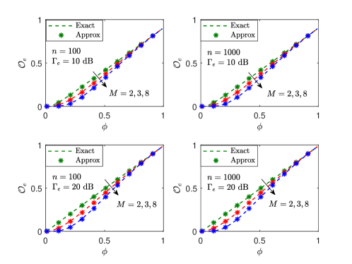
The threshold mentioned in the last step is related to . This step further determines the optimal which is independent of and . For tractability, consider an asymptotically large blocklength and exploit the tail property of the -function, then the information leakage probability is approximated as [33]
| (31) |
Fig. 5 shows that the approximate is extremely close to the exact value for quite a wide range of , , , and , and it then can be adopted to facilitate the subsequent analysis and optimization. Revisiting with , the following lemma is obtained.
Lemma 2 ([38])
, , and .
IV-A4 Solving
This step gives the optimal blocklength that maximizes secrecy throughput.
Theorem 6
is optimal for maximizing in (26).
Proof 11
IV-A5 Solving
By now, the secrecy throughput conditioned on is given by
| (34) |
where and with . For notational simplicity, has been dropped from . Obviously, maximizing is equivalent to maximizing the following function:
| (35) |
Theorem 7
Proof 12
Please refer to Appendix -F.
Theorem 7 shows that, the naive beamforming scheme without injecting any AN is optimal for maximizing the secrecy throughput only when the quality of the main channel is good enough and meanwhile the quality of the wiretap channel is poor or a high information leakage probability is acceptable. Using the derivative rule for implicit functions with (37) proves that , which suggests that in order to support a higher secrecy rate, a larger fraction of power should be allocated to the information signal although at the cost of a larger required rate redundancy.
For a robust design perspective, a worst-case scenario is considered by ignoring Eve’s thermal noise, i.e., in (31), such that with . It is seen from (37) that is a function of and , and the monotonicity of is revealed as below.
Corollary 5
For the worst case , the optimal power allocation is non-decreasing w.r.t. and . Moreover, and .
Proof 13
Please refer to Appendix -G.
Corollary 5 suggests that when the quality of the main channel improves (i.e., a larger ) or the secrecy requirement is relaxed (i.e., a larger ), it would be more appealing to use a higher signal power to promote the main channel than to increase the AN power to degrade the wiretap channel. This is because that the main channel becomes the dominate factor to the improvement of secrecy throughput. Different from Theorem 7 where can be achieved, the optimal here only can be increased up to as due to Eve’s background noise being ignored. Besides, it is unsurprising that for since there is no secrecy requirement.
IV-A6 Solving
For any given power allocation , it can be proved that the secrecy throughput is a concave function of the secrecy rate as done in Theorem 2. Hence, the optimal maximizing is given by (12) and a closed-form lower bound on can be found in (14). Eventually, problem (26) can be addressed via an alternating optimization (AO) method, which is summarized in Algorithm 1. In addition, at the high regime, the optimal is independent of , and hence a global optimal pair is obtained for maximizing .
Fig. 6 illustrates the optimal power allocation and the corresponding maximal secrecy throughput for varying secrecy rate . The maximal is concave on , which guarantees the global optimality of the solution and the convergence of the proposed AO algorithm. The optimal increases with and , which verifies Corollary 5. In addition, the curves of and are truncated after exceeds some critical values. This can be explained similarly as that of Fig. 2. It is shown that increases with the blocklength , although slightly. This is because, increasing will mildly decrease the information leakage probability , thus allowing a larger portion of power to be devoted to transmitting the information-bearing signal.

IV-B Non-Adaptive Optimization Scheme
This subsection examines the secrecy throughput maximization through a non-adaptive design manner for the multi-antenna transmitter case. The problem can be formulated as
| (39a) | ||||
| (39b) | ||||
where is the average successful decoding probability.
The basic idea to solve problem (39) is similar to that of problem (15). Again, the optimal rate redundancy is with given in (4). For the adaptive case, it is known from (IV-A2) that suffices to guarantee a positive secrecy rate with the threshold independent of , and then is optimal for secrecy throughput maximization. As for the non-adaptive one, supporting a certain secrecy rate requires that which is further transformed to
| (40) |
Although herein depends on , it is proved that monotonically decreases with . Hence, is still throughput-optimal for the non-adaptive case. Accordingly, the optimal threshold is . Similar to the proof of Theorem 3, using the maximal blocklength is optimal for maximizing secrecy throughput, regardless of the distribution of . Hence, the optimal blocklength is . Afterwards, the secrecy throughput is calculated from (III-B):
| (41) |
where holds by invoking the CDF of in (29) and computing the integral, with and being the regularized upper incomplete gamma function, with , , , and . Differentiating w.r.t. yields
| (42) |
where and with given in (34). It is verified that the derivative is monotonically decreasing with . In other words, for a fixed , the optimal that maximizes is unique, which is if or otherwise satisfies . Likewise, it is confirmed that the derivative
| (43) |
is first positive and then negative with increasing , and the unique optimal maximizing can be calculated via a bisection method with the equation .

The monotonicity of w.r.t. and is verified in Fig. 7, where, similar to Fig. 6, is given with the optimal or . This implies that the global maximal is practically achieved even by alternatively solving the optimal and . As expected, improves with a larger blocklength and a looser secrecy constraint (a larger ). It is found that first increases and then might decrease with , which means that a moderate is desired to balance the decoding and throughput performance. On the other hand, a larger is required to support an increasing . It is also shown that for a fixed increases with , since a larger improves the decoding performance which then affords a larger . Nevertheless, decreases with in the low regime whereas increases with in the high regime. It can be explained as follows: for a low , the rate redundancy has a great impact on the decoding performance, and hence the AN power should be increased as increases to better combat the eavesdropper; in contrast, for a large , the decoding correctness is more affected by the main channel quality, which requires a larger signal power to maintain a high decoding probability.
Proposition 1
For the high average channel gain , in (IV-B) is approximated as
| (44) |
Proof 14
Please refer to Appendix -H.
Proposition 1 shows that for a high average channel gain, the secrecy throughput becomes independent of the blocklength. In consequence, the optimal and maximizing in (44) admit the following closed-form approximations [22, (19), (20)]
| (45) | ||||
| (46) |
Fig. 8 illustrates the influence of the number of transmit antennas on the maximal secrecy throughput for both adaptive and non-adaptive schemes and the relative secrecy throughput gain . It is not surprising that deploying more transmit antennas can significantly improve the secrecy throughput for both schemes. Similar to the observation in Fig. 4, both and increase with and , but the benefit to brought by a larger is nearly negligible. The right-hand-side subgraph shows that drops sharply as increases but grows for a larger and a smaller . This indicates that the superiority of the adaptive scheme over its non-adaptive counterpart is more pronounced for the scenarios requiring a large blocklengh, having few transmit antennas, suffering from a stringent secrecy constraint, etc; otherwise, the non-adaptive scheme might be appealing because of the low-complexity off-line design.

IV-C A Note on Multi-Antenna Eve
This subsection examines the secure transmission in the presence of an Eve with antennas. Assume that Eve employs the minimum mean-squared error (MMSE) receiver, and then the CDF of Eve’s SINR under the null-space AN scheme can be given as [24]:
| (47) |
where
| (48) |
The information leakage probability is obtained by substituting (47) into (50), and the secrecy throughput can be optimized similarly as described in the above two subsections.
By ignoring the receiver noise at Eve, i.e., considering Eve’s transmit power , one can obtain . Furthermore, if Eve has more antennas than Alice, i.e., , one have , , and accordingly . This means, when , Eve with enough antennas can completely eliminate all the AN signals with an MMSE receiver such that her SNR will approach infinity. As a consequence, the SOP constraint can no longer be satisfied for any chosen rate redundancy, and no positive secrecy rate can be achieved from the perspective of secrecy outage. In other words, the null-space AN scheme can safeguard secure transmissions well for the finite blocklength regime only when the eavesdropper has fewer antennas than the transmitter, and this conclusion is the same as that for the infinite blocklength case.
V Conclusions
This paper investigated the design of secure transmissions in slow fading channels, where secrecy encoding with finite blocklength was employed to confront the eavesdropper. Both adaptive and non-adaptive schemes were devised to maximize the secrecy throughput, providing the optimal threshold of the on-off transmission policy, blocklength, code rates, and power allocation of the AN scheme. Theoretical and numerical results showed that, under the on-off policy, increasing the blocklength can simultaneously enhance the reliability and secrecy, and thus the secrecy throughput is maximized when using the maximal blocklength. In addition, since an overly large secrecy rate will significantly decrease the successful decoding probability thus lowering the secrecy throughput, there exists a critical secrecy rate, but not as large as possible, that can achieve the maximal secrecy throughput.
-A Proof of Lemma 1
For tractability, a piece-wise linear approximation approach is leveraged to approximate the -function given in (2), i.e., for [32, 33],333 This approximation has been extensively applied to the finite-blocklength scenarios, and its accuracy has been well validated. with
| (49) |
where , , , and .444Generally, or should be satisfied to ensure a positive . With (49), the information leakage probability defined in (4) is calculated as
| (50) |
where is the CDF of for , and the last equality in (50) follows from invoking (49) and using partial integration. Next, treat as a continuous variable. As satisfies , the derivative is obtained by using the derivative rule for implicit functions [23] with , i.e.:
| (51) |
First, it can be proved that by noting that and
where follows from the partial integration. The next step is to determine the sign of . The first and second derivatives of w.r.t. are respectively given by
| (52) | ||||
| (53) |
It is easy to see as decreases with and . This indicates that increases with such that . Combining and yields . With and in (51), is obtained, which completes the proof.
-B Proof of Theorem 1
The derivative of w.r.t. is given by
| (54) |
which follows from the derivative . Plugging , as shown in Lemma 1, into (54) yields . For a fixed in (10), it is directly concluded that , which means that monotonically increases with . Since is an integer, is maximized at the maximal integer of , i.e., , which completes the proof.
-C Proof of Theorem 2
From (13), it is easy to prove that , i.e., is concave on . It is verified that . As a result, is maximized at the boundary if or otherwise at the unique zero-crossing of , i.e., . Next, the condition is equivalently transformed to that does not exceed a critical value . Let . It can be readily confirmed that , and decreases with if or otherwise increases with . This leads to . An upper bound for is further provided by realizing that . Then, can be quickly calculated using the bisection method with in the range . This completes the proof.
-D Proof of Theorem 4
First, display the derivative in a recursive form with in (20). Then, the derivative is given by , with presented in (21). It is easily proved that when and as . The key step of the proof is to argue that monotonically decreases with , which guarantees a unique zero-crossing of within . In other words, initially increases and then decreases with and reaches the maximum when arrives at the unique zero-crossing of . To this end, it is necessary to calculate the derivative :
| (55) |
where . To proceed, the following lemma is introduced.
Lemma 3
decreases with and satisfies
| (56) |
Proof 15
Define such that . The monotonicity of w.r.t. is due to . The lower bound of is obtained from and the upper bound follows from and .
With the lower bound of given in (56), it can be readily proved that such that the term in (55) is negative. Besides, since directly yields , one only needs to discuss the situation and prove that
| (57) |
where is due to , holds by invoking Lemma 3 along with algebraic manipulations, and derives from as .
-E Proof of Theorem 5
First fix , and it is clear that the term in (28) increases with as increases with . It is also verified that the term in (28) increases with by computing the derivative of w.r.t. :
| (58) |
where holds by substituting for , follows from the inequality with , and is due to . Hence, in (28) increases with as decreases with . This indicates, is optimal for maximizing for any given and and is also optimal for maximizing .
-F Proof of Theorem 7
Let , where and such that and . Rewrite the second derivative as with given by (-F) at the top of this page, where holds by recalling the definition and invoking the result from Lemma 2, follows from plugging , using the inequality , and omitting the term , holds by substituting into , and is established after some manipulation operations and by discarding the negative term noting that . As indicated by (-F) that is concave on , is maximized at if or otherwise at the unique zero-crossing of . Besides, is equivalent to in (38). Clearly, must be ensured to yield a positive , with which it can be verified that increases with . As a consequence, can be transformed to an explicit form with relation to , namely, . This completes the proof.
| (59) |
-G Proof of Corollary 5
-H Proof of Proposition 1
References
- [1]
- [2] M. Bloch and J. Barros, Physical-Layer Security: From Information Theory to Security Engineering. Cambridge University Press, 2011.
- [3] A. Mukherjee, S. A. A. Fakoorian, J. Huang, and A. L. Swindlehurst, “Principles of physical layer security in multiuser wireless networks: A survey,” IEEE Commun. Surveys Tuts., vol. 16, no. 3, pp. 1550–1573, Aug. 2014.
- [4] N. Yang, L. Wang, G. Geraci, M. Elkashlan, J. Yuan, and M. D. Renzo, “Safeguarding 5G wireless communication networks using physical layer security,” IEEE Commun. Mag., vol. 53, no. 4, pp. 20–27, Apr. 2015.
- [5] Y. Zou, X. Wang, and L. Hanzo, “A survey on wireless security: Technical challenges, recent advances and future trends,” Proc. IEEE, vol. 104, no. 9, pp. 1727–1765, Sep. 2016.
- [6] H.-M. Wang and T.-X. Zheng, Physical Layer Security in Random Cellular Networks. Singapore: Springer, Oct. 2016.
- [7] X. Chen, D. W. K. Ng, W. Gerstacker, and H.-H. Chen, “A survey on multiple-antenna techniques for physical layer security,” IEEE Commun. Surveys Tuts., vol. 19, no. 2, pp. 1027–1053, 2nd Quart., 2017.
- [8] Y. Wu, A. Khisti, C. Xiao, G. Caire, K.-K. Wong, and Xiqi Gao, “A survey of physical layer security techniques for 5G wireless networks and challenges ahead,” IEEE J. Sel. Areas Commun., vol. 36, no. 4, pp. 679–695, Apr. 2018.
- [9] Y. Deng, L. Wang, S. A. R. Zaidi, J. Yuan, and M. Elkashlan, “Artificial-noise aided secure transmission in large scale spectrum sharing networks,” IEEE Trans. Commun., vol. 64, no. 5, pp. 2116–2129, May 2016.
- [10] Y. Liu, Z. Qin, M. Elkashlan, Y. Gao, and L. Hanzo, “Enhancing the physical layer security of non-orthogonal multiple access in large-scale networks,” IEEE Trans. Wireless Commun., vol. 16, no. 3, pp. 1656–1672, Mar. 2017.
- [11] W. Wang, K. C. Teh, and K. H. Li, “Artificial noise aided physical layer security in multi-antenna small-cell networks,” IEEE Trans. Inf. Forensics Security, vol. 12, no. 6, pp. 1470–1482, Jun. 2017.
- [12] Z. Ding, Z. Zhao, M. Peng, and H. V. Poor, “On the spectral efficiency and security enhancements of NOMA assisted multicast-unicast streaming,” IEEE Trans. Commun., vol. 65, no. 7, pp. 3151–3163, Jul. 2017.
- [13] S. Yan, N. Yang, I. Land, R. Malaney, J. Yuan, “Three artificial-noise-aided secure transmission schemes in wiretap channels,” IEEE Trans. Veh. Technol., vol. 67, no. 4, pp. 3669–3673, Apr. 2018.
- [14] A. D. Wyner, “The wire-tap channel,” Bell Syst. Tech. J., vol. 54, no. 8, pp. 1355–1387, Oct. 1975.
- [15] G. Durisi, T. Koch, and P. Popovski, “Toward massive, ultrareliable, and low-latency wireless communication with short packets,” Proc. IEEE, vol. 104, no. 9, pp. 1711–1726, Sep. 2016.
- [16] V. W. S. Wong, R. Schober, D. W. K. Ng, and L.-C. Wang, Key Technologies for 5G Wireless Systems. Cambridge, UK: Cambridge University Press, Apr. 2017.
- [17] C. Cao, H. Li, Z. Hu, W. Liu, and X. Zhang, “Physical-layer secrecy performance in finite blocklength case,” in Proc. IEEE Global Commun. Conf. (GLOBECOM), San Diego, CA, USA, Dec 2015, pp. 1–6.
- [18] W. Yang, R. F. Schaefer, and H. V. Poor, “Finite-blocklength bounds for wiretap channels,” in Proc. IEEE Int. Symp. Inf. Theory (ISIT), Barcelona, Spain, Jul. 2016, pp. 3087–3091.
- [19] M. H. Yassaee, M. R. Aref, and A. Gohari, “Non-asymptotic output statistics of random binning and its applications,” in Proc. IEEE Int. Symp. Inf. Theory (ISIT), Istanbul, Turkey, Jul. 2013, pp. 1849–1853.
- [20] V. Y. F. Tan, “Achievable second-order coding rates for the wiretap channel,” in Proc. IEEE Int. Conf. Comm. Syst. (ICCS), Singapore, Nov. 2012, pp. 65–69.
- [21] W. Yang, R. F. Schaefer, and H. V. Poor, “Secrecy-reliability tradeoff for semi-deterministic wiretap channels at finite blocklength,” in Proc. IEEE Int. Symp. Inf. Theory (ISIT), Aachen, Germany, Jun. 2017, pp. 2133–2137.
- [22] X. Zhang, X. Zhou, and M. R. McKay, “On the design of artificial-noise-aided secure multi-antenna transmission in slow fading channels,” IEEE Trans. Veh. Technol., vol. 62, no. 5, pp. 2170–2181, Jun. 2013.
- [23] T.-X. Zheng, H.-M. Wang, J. Yuan, D. Towsley, and M. H. Lee, “Multi-antenna transmission with artificial noise against randomly distributed eavesdroppers,” IEEE Trans. Commun., vol. 63, no. 11, pp. 4347–4362, Nov. 2015.
- [24] T.-X. Zheng, H.-M. Wang, Q. Yang, and M. H. Lee, “Safeguarding decentralized wireless networks using full-duplex jamming receivers,” IEEE Trans. Wireless Commun., vol. 16, no. 1, pp. 278–292, Jan. 2017.
- [25] T.-X. Zheng, H.-M. Wang, J. Yuan, Z. Han, and M. H. Lee, “Physical layer security in wireless ad hoc networks under a hybrid full-/half-duplex receiver deployment strategy,” IEEE Trans. Wireless Commun., vol. 16, no. 6, pp. 3827–3839, Jun. 2017.
- [26] T.-X. Zheng, H.-M. Wang, and J. Yuan, “Secure and energy-efficient transmissions in cache-enabled heterogeneous cellular networks: Performance analysis and optimization,” IEEE Trans. Commun., vol. 66, no. 11, pp. 5554–5567, Nov. 2018.
- [27] J. Farhat, G. Brante, and R. D. Souza, “Secure throughput optimization of selective decode-and-forward with finite blocklength,” in Proc. IEEE Veh. Technol. Conf. (VTC Spring), Porto, Portugal, Jul. 2018, pp. 1–5.
- [28] W. K. Harrison, J. Almeida, M.R. Bloch, S.W. McLaughlin, and J. Barros, “Coding for secrecy: An overview of error-control coding techniques for physical-layer security,” IEEE Signal Process. Mag., vol. 30, no. 5, pp. 41–50, Sep. 2013.
- [29] D. P. Bertsekas and R. G. Gallager, Data Networks, 2nd ed. Englewood Cliffs, NJ, USA: Prentice–Hall, 1992.
- [30] Y. Polyanskiy, H. Poor, and S. Verdu, “Channel coding rate in the finite blocklength regime,” IEEE Trans. Inf. Theory, vol. 56, no. 5, pp. 2307–2359, May 2010.
- [31] P. Gopala, L. Lai, and H. El Gamal, “On the secrecy capacity of fading channels,” IEEE Trans. Inf. Theory, vol. 54, no. 10, pp. 4687–4698, Oct. 2008.
- [32] B. Makki, T. Svensson and M. Zorzi, “Finite block-length analysis of the incremental redundancy HARQ,” IEEE Wireless Commun. Lett., vol. 3, no. 5, pp. 529–532, Oct. 2014.
- [33] B. Makki, T. Svensson, and M. Zorzi, “Wireless energy and information transmission using feedback: Infinite and finite block-length analysis,” IEEE Trans. Commun., vol. 64, no. 12, pp. 5304–5318, Dec. 2016.
- [34] S. Goel and R. Negi, “Guaranteeing secrecy using artificial noise,” IEEE Trans. Wireless Commun., vol. 7, no. 6, pp. 2180–2189, Jun. 2008.
- [35] A. Khisti and G. W. Wornell, “Secure transmission with multiple antennas I: The MISOME wiretap channel,” IEEE Trans. Inf. Theory, vol. 56, no. 7, pp. 3088–3104, Jul. 2010.
- [36] A. Khisti and G. W. Wornell, “Secure transmission with multiple antennas–part II: The MIMOME wiretap channel,” IEEE Trans. Inf. Theory, vol. 56, no. 11, pp. 5515–5532, Nov. 2010.
- [37] P.-H. Lin, S.-H. Lai, S.-C. Lin, and H.-J. Su, “On secrecy rate of the generalized artificial-noise assisted secure beamforming for wiretap channels,” IEEE J. Sel. Areas Commun., vol. 31, no. 9, pp. 1728–1740, Sep. 2013.
- [38] B. Wang, P. Mu, and Z. Li, “Secrecy rate maximization with artificial-noise-aided beamforming for MISO wiretap channels under secrecy outage constraint,” IEEE Commun. Lett., vol. 19, no. 1, pp. 18–21, Jan. 2015.
- [39] F. W. J. Olver, D. W. Lozier, R. F. Boisvert, and C. W. Clark, NIST Handbook of Mathematical Functions, Cambridge, UK: Cambridge University Press, 2010.