This paper was converted on www.awesomepapers.org from LaTeX by an anonymous user.
Want to know more? Visit the Converter page.

Physical Layer Security Enhancement With Reconfigurable Intelligent Surface-Aided Networks

Jiayi Zhang, , Hongyang Du, Qiang Sun, Bo Ai, ,
and Derrick Wing Kwan Ng
J. Zhang and Q. Sun are with the School of Information Science and Technology, Nantong University, Nantong 226019, China. J. Zhang is also with with the School of Electronic and Information Engineering, Beijing Jiaotong University, Beijing 100044, P. R. China. (e-mail: [email protected]).H. Du is with the School of Electronic and Information Engineering, Beijing Jiaotong University, Beijing 100044, P. R. China. (e-mail: [email protected])B. Ai is with the State Key Laboratory of Rail Traffic Control and Safety, Beijing Jiaotong University, Beijing 100044, China (e-mail: [email protected]).D. W. K. Ng is with the School of Electrical Engineering and Telecommunications, University of New South Wales, NSW 2052, Australia. (e-mail: [email protected]).
Abstract

Reconfigurable intelligent surface (RIS)-aided wireless communications have drawn significant attention recently. We study the physical layer security of the downlink RIS-aided transmission framework for randomly located users in the presence of a multi-antenna eavesdropper. To show the advantages of RIS-aided networks, we consider two practical scenarios: Communication with and without RIS. In both cases, we apply the stochastic geometry theory to derive exact probability density function (PDF) and cumulative distribution function (CDF) of the received signal-to-interference-plus-noise ratio. Furthermore, the obtained PDF and CDF are exploited to evaluate important security performance of wireless communication including the secrecy outage probability, the probability of nonzero secrecy capacity, and the average secrecy rate. Monte-Carlo simulations are subsequently conducted to validate the accuracy of our analytical results. Compared with traditional MIMO systems, the RIS-aided system offers better performance in terms of physical layer security. In particular, the security performance is improved significantly by increasing the number of reflecting elements equipped in a RIS. However, adopting RIS equipped with a small number of reflecting elements cannot improve the system performance when the path loss of NLoS is small.

Index Terms:
Fisher-Snedecor \mathcal{F}-distribution, multiple-input multiple-output, reconfigurable intelligent surface, stochastic geometry.

I Introduction

Recently, reconfigurable intelligent surface (RIS) has been proposed as a promising technique as it can achieve high spectral-/energy-efficiency through adaptively controlling the wireless signal propagation environment [1]. Specifically, RIS is a planar array which comprises a large number of nearly passive reflecting elements. By equipping the RIS with a controller, each element of the RIS can independently introduce a phase shift on the reflected signal. Besides, a RIS can be easily coated on existing infrastructures such as walls of buildings, facilitating low-cost and low-complexity implementation. By smartly adjusting the phase shifts induced by all the reflecting elements, the RIS can bring various potential advantages to the system such as enriching the channel by deliberately introducing more multi-paths, increasing the coverage area, or beamforming, while consuming very low amount of energy due to the passive nature of its elements [2]. Recently, RIS has been introduced into many wireless communication systems. For instance, the authors in [3] studied a RIS-aided single-user multiple-input single-output (MISO) system and optimized the introduced phase shifts to maximize the total received signal power at the users. In [4], various designs were proposed for both the transmit power allocation at a base station (BS) and the phases introduced by the RIS elements to maximize the energy and the spectral efficiency of a RIS-aided multi-user MISO system. Besides, the authors of [5] considered a downlink (DL) multiuser communication system where the signal-to-interference-plus noise ratio (SINR) was maximized for given phase shifts introduced by a RIS.

In practice, communication security is always a fundamental problem in wireless networks due to its broadcast nature. Besides traditional encryption methods adopted in the application layer, physical layer security (PLS) [6, 7, 8] serves as an alternative for providing secure communication in fast access fifth-generation (5G) networks. Furthermore, PLS can achieve high-quality safety performance without requiring actual key distribution, which is a perfect match with the requirements of 5G. To fully exploit the advantages of 5G, multi-antenna technology has become a powerful tool for enhancing the PLS in wireless fading networks, e.g. [9, 10, 11, 12, 13, 14, 15]. In particular, with the degrees of freedom provided by multiple antennas, a transmitter can steer its beamforming direction to exploit the maximum directivity gain to reduce the potential of signal leakage to eavesdroppers. However, there are only a few works considering the PLS in the emerging RIS-based communication systems, despite its great importance for modern wireless systems. For example, a RIS-aided secure communication system was investigated in [16, 17] but their communication systems only consist of a transmitter, one legitimate receiver, single eavesdropper, and a RIS with limited practical applications. Furthermore, authors in [18] studied a DL MISO broadcast system where a BS transmits independent data streams to multiple legitimate receivers securely in the existence of multiple eavesdroppers. In order to conceive a practical RIS framework, user positions have to be taken into account using stochastic geometry for analyzing the system performance. In fact, stochastic geometry is an efficient mathematical tool for capturing the topological randomness of networks [19, 20]. However, there are only a few works studying the impact of user-locations on the security performance.

Motivated by the aforementioned reasons, in this paper, we study the security performance of a RIS-aided DL multiple-input multiple-output (MIMO) system for randomly located roaming multi-antenna users in the presence of a multi-antenna eavesdropper. Moreover, we aim to answer a fundamental question “How much improvement can RIS bring to physical layer security in wireless communications?”. The main contributions of this paper are summarized as follows:

  • To show the advantages of exploiting RIS to enhance the PLS in wireless communications, we consider two practical scenarios: RIS is adopted and its absence. For each case, we derive the exact closed-form expressions of SINR and its PDF and CDF, respectively. Furthermore, considering a general set-up when the direct links between the BS and the RIS-aided users exist, we obtain the CDF and outage probability (OP) expressions.

  • Exploiting the tools from stochastic geometry, we propose a novel PLS analysis framework of RIS-aided communication systems. Novel expressions are derived to characterize the PLS performance, namely the secrecy outage probability (SOP), the probability of nonzero secrecy capacity (PNSC), and the average secrecy rate (ASR). The derived results can provide insights, i.e., the security performance is improved significantly by increasing the number of reflecting elements.

  • We derive highly accurate and simplified closed-form approximations of the CDF expressions of SINR for both scenarios. Furthermore, we present an asymptotic OP analysis in the high-SNR regime. The derived results show that adopting RIS equipped with a small number of reflecting elements cannot improve the system performance if the path loss of NLoS is small.

The remainder of the paper is organized as follows. In Section II, we introduce the system model of the RIS-aided DL MIMO communication system and derive the exact closed-form of PDF and CDF expressions of SINR for users and the eavesdropper. Section III formulates the security performance analysis in two scenarios and present the corresponding exact expressions of the performance. In Section IV, we derive the approximations to the statistics of SINR in two scenarios, and analyze the OP in high-SINR regime. Section V presents the CDF and OP of scenario 2 when the direct links exist between BS and RIS-aided users. Section VI shows the simulation results and the accuracy of the obtained expressions is validated via Monte-Carlo simulations. Finally, Section VII concludes this paper.

Mathematical notations: A list of mathematical symbols and functions most frequently used in this paper is available in Table I.

TABLE I: MATHEMATICAL SYMBOLS AND FUNCTIONS
υ\upsilon A subscript which denotes different links. υ=u1,,uN,ue,uR\upsilon=u_{1},\cdots,u_{N},u_{e},u_{R} denotes the signal is sent by the BS, and destinations are NN users, the eavesdropper, and the RIS, respectively. υ=uRu1,,uRuN,uRue\upsilon=u_{R}-u_{1},\cdots,u_{R}-u_{N},u_{R}-u_{e} denotes the signal is reflected by the RIS, and the destinations are NN users and the eavesdropper, respectively.
σ\sigma A subscript which denotes different kinds of path loss. σ=L\sigma={\rm L} denotes the LoS links, σ=NL\sigma={\rm NL} denotes the NLoS links.
κ\kappa A subscript which denotes different antennas.
𝔼[]{\mathbb{E}}[\cdot] The mathematical expectation.
r2r_{2} The radius of the disc.
𝐇H{\bf H}^{\rm H} Conjugate transpose.
𝐇T{\bf H}^{\rm T} Transpose.
x×y{{\mathbb{C}}^{x\times y}} The space of x×yx\times y complex-valued matrices.
F\|\cdot\|_{F} The Frobenius norm.
jj j=1j=\sqrt{-1}
{Δi}i=1L\left\{{{\Delta_{i}}}\right\}_{i=1}^{L} {Δi}i=1L\left\{{{\Delta_{i}}}\right\}_{i=1}^{L} denotes Δ1,Δ2,,ΔL{\Delta_{1}},{\Delta_{2}},\cdots,{\Delta_{L}}.
Γ()\Gamma\left(\cdot\right) Gamma function [21, eq. (8.310/1)]
B(,){B\left({\cdot,\cdot}\right)} Beta function [21, Eq. (8.384.1)]
F12(,;;){}_{2}{F_{1}}\!\left({\!\cdot,\cdot;\cdot;\cdot\!}\right) Hypergeometric function [21, Eq. (9.111)]
Gm,np,q()G\,\begin{subarray}{c}m,n\\ p,q\end{subarray}(\cdot) Meijer’s GG-function [21, eq. (9.301)]

II System Model And Preliminaries

II-A System Description

Refer to caption
Figure 1: Two practical scenarios: Communication without (left hand side) and with RIS (right hand side).

Let us consider the DL MIMO-RIS system and assume that a BS equipped with MM transmit antennas (TAs) communicates with NN users each of which is equipped with KK receive antennas (RAs). a RIS is installed between the BS and the users for assisting end-to-end communication. By jointly optimizing the transmit precoding at the BS and the reflect phase shifts at the RIS according to the wireless channel conditions, the reflected signals can be added constructively at the desired receiver to enhance the received signal power, which can potentially yield a secure transmission [22]. In addition, a malicious eavesdropper who is equipped with KK RAs aims to eavesdrop the information of the desired user. We assume that the number of reflecting elements on the RIS is LL. The RIS is equipped with a controller to coordinate between the BS and the RIS for both channel acquisition and data transmission [3]. As such, the signal received from the BS can be manipulated by the RIS via adjusting the phase shifts and amplitude coefficients of the RIS elements.

On the other hand, various practical approaches have been proposed in the literature for the channel estimation of RIS-aided links [23, 24, 25]. Thus, we can assume that the global channel state information (CSI) of users is perfectly known for joint design of beamforming [26]. The CSI of the eavesdropper is typically unavailable as the eavesdropper is passive to hide its existence. Therefore, the passive eavesdropping scenario is considered [27]. To quantify the performance of such a RIS-aided communication system, we adopt SOP, PNSC, and ASR as performance metrics of interested.

In particularly, we assume that the users are located on a disc with a radius r2r_{2} according to homogeneous Poisson point processes (HPPP) [28] with density λ\lambda and the eavesdropper will try to choose a position that is close to the legitimate user.

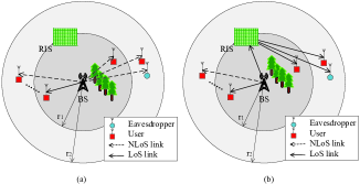
In practice, the direct transmission link between the BS and the users may be blocked by trees or buildings. Such assumption is applicable for 5G and mmWave communication systems that are known to suffer from high path and penetration losses resulting in signal blockages. In order to unveil the benefits in adopting the RIS, we consider the following two practice of communication scenarios:

  • As shown in Fig. 1 (a), for the first scenario, RIS is not adopted for enhancing the PLS and the quality of wireless communication. Specifically, both LoS and NLoS links exist in our system. Without loss of generality, we focus our attention on user nn. We use dυ,σd_{\upsilon,\sigma} to denote the distance between the BS and user nn (n=1,,N)(n=1,\cdots,N). According to Table I, we have υ=un\upsilon=u_{n}, σ=L\sigma={\rm L} for LoS links and υ=un\upsilon=u_{n}, σ=NL\sigma={\rm NL} for NLoS links.

  • For the second scenario, a RIS is deployed to leverage the LoS components with respect to both the BS and the users to assist their end-to-end communication of Fig. 1 (b). Thus, the NLoS users in scenario 1 now can communicate with BS through two LoS links with the help of RIS. Moreover, the locations of the BS and the RIS are fixed, hence we assume that the distance between the BS and the RIS is known and denoted by duR,Ld_{u_{R},{\rm L}}. In addition, the distance between the RIS and user nn is denoted by duRun,Ld_{u_{R}-u_{n},{\rm L}}.

II-B Blockage Model

A blockage model was proposed in [29], which can be regarded as an accurate approximation of the statistical blockage model [30] and incorporates the LoS ball model proposed in [31] as a special case. In the considered system model, we adopt the blockage model to divide the users process in the spherical region around the BS into two independent HPPPs: LoS users process and NLoS users process. In particular, we define qL(r){q_{L}}(r) as the probability that a link of length rr is LoS. Each access link of separation rr is assumed to be LoS with probability B1B_{1} if rr1r\leq r_{1} and 0 otherwise:

qL(r)={B1,ifrr10,otherwise,{q_{L}}(r)=\left\{{\begin{array}[]{*{20}{l}}{B_{1},}&{{\rm{if}}\quad r\leq r_{1}}\\ {0,}&{{\rm{otherwise}}}\end{array}}\right., (1)

where 0B110\leq B_{1}\leq 1. The parameter B1B_{1} can be interpreted as the average LoS area in a circular ball with a radius of r1r_{1} around the BS.

II-C User Model

Let us assume that the users are located according to a HPPP within the disc shown as Fig. 1. The PDF of the user locations have been derived as [32, eq. (30)]. As a result, the CDF of the user locations is given by

FR(r)=r2(r22r02)r02(r22r02),ifr0<r<R,{F_{R}}(r)=\frac{{{r^{2}}}}{{\left({{r_{2}}^{2}-r_{0}^{2}}\right)}}-\frac{{r_{0}^{2}}}{{\left({{r_{2}}^{2}-r_{0}^{2}}\right)}},\qquad{\rm{if}}\quad{r_{0}}<r<R, (2)

where r0r_{0} is the minimum distance which is used to avoid encountering a singularity [33]. Thus, the probability of the distance between the user and the BS is less than r1r_{1} can be expressed as

B2Pr(rr1)=FR(r1)=r12(r22r02)r02(r22r02).{B_{2}}\triangleq{\rm{Pr}}\left({r\leq{r_{1}}}\right)={F_{R}}({r_{1}})=\frac{{r_{1}^{2}}}{{\left({{r_{2}}^{2}-r_{0}^{2}}\right)}}-\frac{{r_{0}^{2}}}{{\left({{r_{2}}^{2}-r_{0}^{2}}\right)}}. (3)

II-D Path Loss Model

For the first communication scenario without a RIS, different path loss equations are applied to model the LoS and NLoS links as [29, 31]

L(d)={dun,Lα1,dun,NLα2,ifBSusernlinkisLoSlink.ifBSusernlinkisNLoSlink,L\left(d\right){=}\left\{{\begin{array}[]{*{20}{c}}\!\!\!{{d_{u_{n},{\rm L}}^{-{\alpha_{1}}}}},\!\!\!\\ \!\!\!{{d_{u_{n},{\rm NL}}^{-{\alpha_{2}}}}},\!\!\!\!\end{array}}\right.\begin{array}[]{*{20}{c}}\!\!\!\!\!{{\rm{if\>BS}}\to{\rm{user\>{\it n}\>link\>is\>LoS\>link.}}}\\ {{\rm{if\>BS}}\to{\rm{user\>{\it n}\>link\>is\>NLoS\>link,}}}\end{array} (4)

where α1{\alpha_{1}} and α2{\alpha_{2}} are the LoS and NLoS path loss exponents, respectively. Typical values of α1{\alpha_{1}} and α2{\alpha_{2}} are defined in [34, Table 1], while α1<α2{\alpha_{1}}<{\alpha_{2}} hold in general.

For the second communication scenario with the assistance by the RIS, recently, the free-space path loss models of RIS-aided wireless communications are developed for different situations in [35, Proposition 1]. Authors in [35] proposed that the free-space path loss of RIS-aided communications is proportional to (duR,LduRun,L)2{(d_{u_{R},{\rm L}}d_{u_{R}-u_{n},{\rm L}})}^{2} in the far field case. Thus, we obtain

L(duR,L,duRun,L)=CL1CL2duR,L2duRun,L2,L\left({{d_{u_{R},{\rm L}}},{d_{u_{R}-u_{n},{\rm L}}}}\right)=C_{L_{1}}C_{L_{2}}d_{u_{R},{\rm L}}^{-2}d_{u_{R}-u_{n},{\rm L}}^{-2}, (5)

where CL1C_{L_{1}} and CL2C_{L_{2}} denote the path loss intercepts of BS-RIS and RIS-user links, respectively.

II-E Small-Scale Fading

To unify the system performance with different channel environment, generalized fading distributions have been proposed that include the most common fading distributions as special cases [36, 37, 8]. It has been shown recently that the Fisher-Snedecor \mathcal{F} composite fading model can provide a more comprehensive modeling and characterization of the simultaneous occurrence of multipath fading and shadowing, which is generally more accurate than most other generalized fading models [38]. Furthermore, the Fisher-Snedecor \mathcal{F} model is more general and includes several fading distributions as special cases, while being more mathematically tractable. For example, authors in [32] conceived a RIS-aided MIMO framework using Nakagami-mm distribution. Note that Fisher-Snedecor \mathcal{F} distribution includes the case of Nakagami-mm distribution for msm_{s}\to\infty as one of its subsequent special cases, such as Rayleigh (m=1)(m=1) and one-sided Gaussian (m=1/2)(m=1/2). Motivated by this, the Fisher-Snedecor \mathcal{F} distribution has been adopted to analyze the RIS-aided systems, i.e., RIS-aided Internet-of-Things networks [39].

To conceive a practical RIS framework, we assume that the small-scale fading of each link follows Fisher-Snedecor \mathcal{F} fading distributions [39]. The channel correlation between RIS elements may exist because the electrical size of RIS’s reflecting elements is between λ/8\lambda/8 and λ/4\lambda/4 in principle, where λ\lambda is a wavelength of the signal [40]. However, it is hard to model the correlation in RIS because a tractable model for capturing such unique characteristics has not been reported in the literature yet. Therefore, we consider a scenario where the correlation is weak enough to be ignored, i.e., the electrical size of RIS’s reflecting elements is larger than λ/4\lambda/4 because the frequency of signals is high [41], [42]. Thus, we can assume that the small scale fading components are independent of each other.

For the first communication scenario, in order to characterize the LoS and NLoS links between the BS and users (eavesdropper), the small-scale fading matrices are defined as

𝐐υ,σ=[q1,1υ,σq1,Mυ,σqK,1υ,σqK,Mυ,σ],{{{\bf Q}}_{\upsilon,\sigma}}=\left[{\begin{array}[]{*{20}{c}}{{q_{1,1}^{\upsilon,\sigma}}}&\cdots&{{q_{1,M}^{\upsilon,\sigma}}}\\ \vdots&\vdots&\vdots\\ {{q_{K,1}^{\upsilon,\sigma}}}&\cdots&{{q_{K,M}^{\upsilon,\sigma}}}\end{array}}\right], (6)

where 𝐐υ,σ{{{\bf Q}}_{\upsilon,\sigma}} (σ=L,NL)(\sigma={\rm L},{\rm NL}) is a K×MK\times M matrix. Letting υ=un\upsilon=u_{n}, we obtain the small-scale fading matrix between the BS and user nn. Using [43, Eq. (5)], the PDF of the elements of (6) can be expressed as

fX(x)=2mm((ms1)Ω)msx2m1B(m,ms)(mr2+(ms1)Ω)m+ms,{f_{X}}(x)=\frac{{2{m^{m}}{{\left({\left({{m_{s}}-1}\right)\Omega}\right)}^{{m_{s}}}}}{{x^{2m-1}}}}{{B\left({m,{m_{s}}}\right)}{{{\left({m{r^{2}}+\left({{m_{s}}-1}\right)\Omega}\right)}^{m+{m_{s}}}}}}, (7)

where Ω=𝔼[r2]\Omega=\mathbb{E}\left[r^{2}\right] is the mean power, mm and msm_{s} are physical parameters which represent the fading severity and shadowing parameters, respectively.

For the second case, the small-scale fading matrices for the LoS links between the BS and users (eavesdropper) are same as the first case. In addition, in order to model the LoS links between the BS and the RIS, the small-scale fading matrix is defined as

𝐐uR,L=[q1,1uR,Lq1,MuR,LqL,1uR,LqL,MuR,L],{{{\bf Q}}_{u_{R},{\rm L}}}=\left[{\begin{array}[]{*{20}{c}}{{q_{1,1}^{u_{R},{\rm L}}}}&\cdots&{{q_{1,M}^{u_{R},{\rm L}}}}\\ \vdots&\vdots&\vdots\\ {{q_{L,1}^{u_{R},{\rm L}}}}&\cdots&{{q_{L,M}^{u_{R},{\rm L}}}}\end{array}}\right], (8)

where 𝐐uR,L{{{\bf Q}}_{u_{R},{\rm L}}} is a L×ML\times M matrix.

In order to model the LoS links between the RIS and users (eavesdropper), the small-scale fading matrices are defined as

𝐐υ,L=[q1,1υ,Lq1,Lυ,LqK,1υ,LqK,Lυ,L],{{{\bf Q}}_{\upsilon,{\rm L}}}=\left[{\begin{array}[]{*{20}{c}}{{q_{1,1}^{\upsilon,{\rm L}}}}&\cdots&{{q_{1,L}^{\upsilon,{\rm L}}}}\\ \vdots&\vdots&\vdots\\ {{q_{K,1}^{\upsilon,{\rm L}}}}&\cdots&{{q_{K,L}^{\upsilon,{\rm L}}}}\end{array}}\right], (9)

where 𝐐υ,L{{{\bf Q}}_{\upsilon,{\rm L}}} is a K×LK\times L matrix. Letting υ=uRun\upsilon=u_{R}-u_{n}, we get the small-scale fading matrix between the RIS and user nn.

II-F Directional Beamforming

Highly directional beamforming antenna arrays are deployed at the BS to compensate the significant path-loss in the considered system. For mathematical tractability and similar to [29, 30], the antenna pattern of users can be approximated by a sectored antenna model in [44] which is given by

𝒢υ,κ(θ)={Gυ,κ,if|θ|θc,gυ,κ,otherwise,(κ=1,,K),{\cal G}_{\upsilon,\kappa}(\theta)=\left\{{\begin{array}[]{*{20}{l}}{{{G}_{\upsilon,\kappa}}},&{{\rm{if}}\>\>|\theta|\leq{\theta_{c}}},\\ {{{g}_{\upsilon,\kappa}}},&{{\rm{otherwise}}},\end{array}}\right.\quad(\kappa=1,\cdots,K), (10)

where θ{\theta}, distributed in [0,2π]\left[{0,2\pi}\right], is the angle between the BS and the user, θc\theta_{c} denotes the beamwidth of the main lobe, for each TA, Gυ,κ{{{G}_{\upsilon,\kappa}}} and gυ,κ{{{g}_{\upsilon,\kappa}}} are respectively the array gains of main and sidelobes. In practice, the BS can adjust their antennas according to the CSI. In the following, we denote the boresight direction of the antennas as 0{0^{\circ}}. For simplifying the performance analysis, different antennas of the authorized users and the malicious eavesdropper are assumed to have same array gains. Thus, without loss of generality, we assume that 𝒢υ,κ=𝒢υ{\cal G}_{\upsilon,\kappa}={\cal G}_{\upsilon}, Gυ,κ=Gυ{G}_{\upsilon,\kappa}={G}_{\upsilon} and gυ,κ=gυ{g}_{\upsilon,\kappa}={g}_{\upsilon}.

II-G SINR Analysis

Let us consider a composite channel model of large-scale and small-scale fading. It is assumed that the distance dυ,σ{d_{\upsilon,\sigma}}, υ=u1,,uN,ue,\upsilon=u_{1},\cdots,u_{N},u_{e}, and σ=L,NL\sigma={\rm L},{\rm NL} are independent but not identically distributed (i.n.i.d.) and the large-scale fading is represented by the path loss. In the DL transmission, the complex baseband transmitted signal at the BS can be then expressed as

x=n=1N𝐩unsun,x=\sum\limits_{n=1}^{N}{{{\bf p}_{u_{n}}}{s_{u_{n}}}}, (11)

where sun{s_{u_{n}}} (n=1,,N)(n=1,\cdots,N) are i.i.d. random variables (RVs) with zero mean and unit variance, denoting the information-bearing symbols of users, and 𝐩unM×1{\bf{p}}_{u_{n}}\in{\mathbb{C}}^{M\times 1} is the corresponding beamforming vector. The transmit power consumed at the BS can be expressed as

P=n=1N𝐩un2.P=\sum\limits_{n=1}^{N}{{{\left\|{{{\bf p}_{u_{n}}}}\right\|}^{{2}}}}. (12)

For the first communication scenario, e.g., Fig. 1 (a), there are both LoS and NLoS links. The signal received by user nn or the eavesdropper from the BS can be expressed as

yυ,σ=\displaystyle y_{\upsilon,\sigma}= GυL(dυ,σ)𝐯υ𝐐υ,σ𝐩υsυ\displaystyle\sqrt{{G_{\upsilon}}L\left({{d_{\upsilon,\sigma}}}\right)}{{\bf{v}}_{\upsilon}}{{\bf{Q}}_{\upsilon,\sigma}}{{\bf p}_{\upsilon}}{s_{\upsilon}}
+GυL(dυ,σ)iυN𝐯υ𝐐υ,σ𝐩isiMultiuserinterference+𝐯υ𝐍0,\displaystyle+\underbrace{\sqrt{{G_{\upsilon}}L\left({{d_{\upsilon,\sigma}}}\right)}\sum\limits_{i\neq\upsilon}^{N}{{{\bf{v}}_{\upsilon}}{{\bf{Q}}_{\upsilon,\sigma}}{\bf p}_{i}{s_{i}}}}_{{\rm{Multi-user\>interference}}}+{{\bf{v}}_{\upsilon}}{{\bf N}_{0}}, (13)

where υ=un,ue\upsilon=u_{n},u_{e}, σ=L,NL\sigma={\rm L},{\rm NL}, 𝐯un1×K{\bf{v}}_{u_{n}}\in{\mathbb{C}}^{1\times K} is the detection vector of user nn, and 𝐍0K×1{\bf N}_{0}\in{\mathbb{C}}^{K\times 1} denotes the additive white Gaussian noise, which is modeled as a realization of a zero-mean complex circularly symmetric Gaussian variable with variance σN2\sigma_{N}^{2}.

For the second communication scenario, e.g., Fig. 1 (b), there are LoS and RIS-aided links. For LoS links, the signal received by the user or the eavesdropper can be obtained by letting σ=L\sigma={\rm L} in (II-G). For RIS-aided links, the signal can be expressed as

yRISυ=GυL(duR,L,duRυ,L)𝐯υ𝐐uRυ,L𝚽𝐐uR,L𝐩υsυ\displaystyle y_{{\rm{RIS}}}^{\upsilon}=\sqrt{{G_{\upsilon}}{L\left({{d_{u_{R},{\rm L}}},{d_{u_{R}-\upsilon,{\rm L}}}}\right)}}{{\bf{v}}_{\upsilon}}{{\bf{Q}}_{u_{R}-\upsilon,{\rm L}}}{\bf{\Phi}}{{\bf{Q}}_{u_{R},{\rm L}}}{{\bf p}_{\upsilon}}{s_{\upsilon}}
+𝐯υ𝐍0+GυL(duR,L,duRυ,L)iυN𝐯υ𝐐uRυ,L𝚽𝐐uR,L𝐩isiMultiuserinterference,\displaystyle+\!{{\bf{v}}_{\upsilon}}{{\bf N}_{0}}\!+\!\!\underbrace{\sqrt{{G_{\upsilon}}{L\!\left(\!{{d_{u_{R},{\rm L}}},{d_{u_{R}\!-\!\upsilon,{\rm L}}}}\!\right)}}\!\sum\limits_{i\neq\upsilon}^{N}\!{{{\bf{v}}_{\upsilon}}{{\bf{Q}}_{u_{R}\!-\!\upsilon,{\rm L}}}{\bf{\Phi}}{{\bf{Q}}_{u_{R},{\rm L}}}{{\bf p}_{i}}{s_{i}}}}_{{\rm{Multi-user\>interference}}}, (14)

where υ=un,ue\upsilon=u_{n},u_{e}, 𝚽=Δdiag[β1ϕ1,β2ϕ2,,βLϕL]{\bf{\Phi}}\buildrel\Delta\over{=}{\mathop{\rm diag}\nolimits}\left[{{\beta_{1}}{\phi_{1}},{\beta_{2}}{\phi_{2}},\cdots,{\beta_{L}}{\phi_{L}}}\right] is a diagonal matrix accounting for the effective phase shift introduced by all the elements of the RIS 111We assume that the phase shifts can be continuously varied in [0,2π)[0,2\pi) to characterize the fundamental performance of RIS. Although using the RIS with discrete phase shifts causes performance loss [45], our results serve as performance upper bounds for the considered system which are still useful for characterizing the fundamental performance of the RIS-aided system., β(0,1]{\beta_{\ell}}\in(0,1] represents the amplitude reflection coefficient, ϕ=exp(jθ){\phi_{\ell}}=\exp\left({j{\theta_{\ell}}}\right), n=1,,Ln=1,\cdots,L, θ[0,2π),{\theta_{\ell}}\in[0,2\pi), denotes the phase shift.

In the literature, numerous methods have been proposed to obtain the effective phase shift introduced by all the elements of the RIS, e.g., [3, 46, 47, 48, 32]. To mitigate the interference at the nthn_{\rm th} user and perform well both in RIS and non-RIS scenarios, we adopt the design of passive beamforming process and the downlink user-detection vectors proposed in [32]. The passive beamforming matrix at RIS can be obtained as [32, eq. (13)]

𝚽=𝐇~1𝐗βmax,{\bf{\Phi}}=\frac{{\bf{\tilde{H}}}^{-1}{\bf{X}}}{\beta_{\max}}, (15)

where βmax\beta_{\max} is obtained by finding the maximum amplitude coefficient, 𝐗{\bf{X}} is the signal sent by BS, and 𝐇~{{{\bf{\tilde{H}}}}} can be formulated from 𝐐uRu1,L𝚽𝐐uR,L{{\bf{Q}}_{u_{R}-u_{1},{\rm L}}}{\bf{\Phi}}{{\bf{Q}}_{u_{R},{\rm L}}}, \cdots, 𝐐uRuN,L𝚽𝐐uR,L{{\bf{Q}}_{u_{R}-u_{N},{\rm L}}}{\bf{\Phi}}{{\bf{Q}}_{u_{R},{\rm L}}} as [32, eq. (9)].

The detection vector of the nthn_{\rm th} user can be written as [32, eq. (19)]

𝐯un=𝐓un𝐱un,{{\bf{v}}_{{u_{n}}}}={{\bf{T}}_{{u_{n}}}}{{\bf{x}}_{{u_{n}}}}, (16)

where 𝐓un{{\bf{T}}_{{u_{n}}}} is derived by the left singular vectors of 𝐇~{{{\bf{\tilde{H}}}}}. With the aid of the classic maximal ratio combining technique, 𝐱un{{\bf{x}}_{{u_{n}}}} can be expressed as

𝐱un=𝐓un𝐇𝐡un|𝐓un𝐇𝐡un|,{{\bf{x}}_{{u_{n}}}}=\frac{{{\bf{T}}_{{u_{n}}}^{\bf{H}}{{\bf{h}}_{{u_{n}}}}}}{{\left|{{\bf{T}}_{{u_{n}}}^{\bf{H}}{{\bf{h}}_{{u_{n}}}}}\right|}}, (17)

where 𝐡un{{\bf{h}}_{{u_{n}}}} is the unth{u_{n}}_{\rm th} column of the effective channel matrix 𝐐uRun,L𝚽𝐐uR,L{{\bf{Q}}_{u_{R}-u_{n},{\rm L}}}{\bf{\Phi}}{{\bf{Q}}_{u_{R},{\rm L}}}. Thus, the SINRs involved in both scenarios can be obtained.

For the first case, the received SINR at user nn and the eavesdropper are denoted as SINRυ,σ{\rm SINR}_{\upsilon,\sigma}, and it can be expressed as222To facilitate effective eavesdropping, the eavesdropper should try to close to BS because the SINR of the eavesdropper increases as due,σd_{u_{e},\sigma} decreases.

SINRυ,σ=𝒢υ𝐡^υ,σF2(dυ,σ)ασpunβmax2Q2σN2,{{\rm SINR}_{\upsilon,\sigma}}=\frac{{{{{\cal G}_{\upsilon}}}\left\|{{{\widehat{\bf{h}}}_{\upsilon,\sigma}}}\right\|_{F}^{2}{{\left({{d_{\upsilon,\sigma}}}\right)}^{-\alpha_{\sigma}}}{p_{u_{n}}}}}{{\beta_{\max}^{2}{Q}^{2}{\sigma_{N}^{2}}}}, (18)

where punp_{u_{n}} denotes the transmit power of the BS for user, QKM1Q\triangleq K-M-1 is the effective antenna gain, and

𝐡^υ,σ=[q1,1υ,σqQ,1υ,σq1,Mυ,σqQ,Mυ,σ]{{{\widehat{\bf{h}}}_{\upsilon,\sigma}}}=\left[{\begin{array}[]{*{20}{c}}{{q_{1,1}^{\upsilon,\sigma}}}\\ \vdots\\ {{q_{Q,{1}}^{\upsilon,\sigma}}}\end{array}\begin{array}[]{*{20}{c}}\cdots\\ \vdots\\ \cdots\end{array}\begin{array}[]{*{20}{c}}{{q_{1,M}^{\upsilon,\sigma}}}\\ \vdots\\ {{q_{Q,M}^{\upsilon,\sigma}}}\end{array}}\right] (19)

is a Q×MQ\times M matrix which denotes the channel gain of user nn. In addition, we can see that the eavesdropper’s SINR is affected by the random directivity gain Gue(θ){G_{{u_{e}}}(\theta)}.

For the second case, the SINR of LoS path can be obtained by letting σ=L\sigma={\rm L} in (18). For the RIS-aided path, with the help of the design of passive beamforming process [32], the SINR with the optimal phase shift design of RIS’s reflector array can be derived as [32, eq. (29)]

SINRυ,RIS=𝒢υCL1CL2𝐡^υ,RISF2(duR,Ldυ,L)2punβmax2Q2σN2,{{\rm SINR}_{\upsilon,{\rm RIS}}}\!=\!\frac{{{\mathcal{G}_{\upsilon}}C_{L_{1}}C_{L_{2}}\left\|{{{\widehat{\bf{h}}}_{\upsilon,{\rm RIS}}}}\right\|_{F}^{2}{{\left({{d_{u_{R},{\rm L}}}{d_{\upsilon,{\rm L}}}}\right)}^{-2}}{p_{u_{n}}}}}{{\beta_{\max}^{2}{Q}^{2}{\sigma_{N}^{2}}}}, (20)

where υ=uRun,uRue\upsilon=u_{R}-u_{n},u_{R}-u_{e}, and

𝐡^υ,RIS=[(q1,1υ,L)(q1,muR,L)(q1,Lυ,L)(qL,muR,L)(qQ,1υ,L)(q1,muR,L)(qQ,Lυ,L)(qL,muR,L)]{{{\widehat{\bf{h}}}_{\upsilon,{\rm RIS}}}}\!=\!\!\left[\!\!{\begin{array}[]{*{20}{c}}{\left({{q_{1,1}^{\upsilon,{\rm L}}}}\right)\cdot\left({{q_{1,m}^{u_{R},{\rm L}}}}\right)}&\cdots&{\left({{q_{1,L}^{\upsilon,{\rm L}}}}\right)\cdot\left({{q_{L,m}^{u_{R},{\rm L}}}}\right)}\\ \vdots&\vdots&\vdots\\ {\left({{q_{Q,1}^{\upsilon,{\rm L}}}}\right)\cdot\left({{q_{1,m}^{u_{R},{\rm L}}}}\right)}&\cdots&{\left({{q_{Q,L}^{\upsilon,{\rm L}}}}\right)\cdot\left({{q_{L,m}^{u_{R},{\rm L}}}}\right)}\end{array}}\!\!\right] (21)

is a Q×LQ\times L matrix.

With the help of (18) and (20), we derive the exact PDF and CDF expressions for each scenario’s SINR in terms of multivariate Fox’s HH-function [49, eq. (A-1)], which are summarized in the following Theorems.

Theorem 1.

For the first communication scenario, let Zυ,σ=SINRυ,σZ_{\upsilon,\sigma}={{\rm SINR}_{\upsilon,\sigma}}, the CDF of Zυ,σZ_{\upsilon,\sigma} is expressed as

FZυ,σ(z)==1QM1Γ(ms)Γ(m)(HCDF1,2HCDF1,0),F_{Z_{\upsilon,\sigma}}(z)=\prod\limits_{\ell=1}^{QM}{\frac{1}{{\Gamma\left({{m_{s_{\ell}}}}\right)\Gamma\left({{m_{\ell}}}\right)}}}(H_{{{\rm CDF}}_{1},2}-H_{{{{\rm CDF}}_{1}},0}), (22)

where HCDF1,H_{{{\rm CDF}}_{1},\hbar} (=0,2)(\hbar=0,2) is derived as (28) at the top of the next page, A1=𝒢υpunβmax2Q2σN2{A_{1}}=\frac{{{\mathcal{G}_{\upsilon}}{p_{{u_{n}}}}}}{{{\beta_{\max}^{2}}{Q^{2}}\sigma_{N}^{2}}}, {m}i=1QM={{mq,nυ,σ}n=1M}q=1Q\left\{{{m_{\ell}}}\right\}_{i=1}^{QM}=\left\{{\left\{{{m_{q,n}^{\upsilon,\sigma}}}\right\}_{n=1}^{M}}\right\}_{q=1}^{Q}{\rm{}}, {ms}i=1QM={{msq,nυ,σ}n=1M}q=1Q\left\{{{m_{{s_{\ell}}}}}\right\}_{i=1}^{QM}\!=\!\left\{{\left\{{{m_{s}}_{q,n}^{\upsilon,\sigma}}\right\}_{n=1}^{M}}\right\}_{q=1}^{Q}{\rm{}}, and {Ω}i=1QM={{Ωq,nυ,σ}n=1M}q=1Q.\left\{{{\Omega_{\ell}}}\right\}_{i=1}^{QM}\!=\!\left\{{\left\{{{\Omega_{q,n}^{\upsilon,\sigma}}}\right\}_{n=1}^{M}}\right\}_{q=1}^{Q}.

HCDF1,2r2(r22r02)ασH1,2:2,1;;2,10,1:1,2;;1,2(A1zrασm1γ¯1(ms11)A1zrασmQMγ¯QM(msQM1)|(12ασ;1,,1):(1,1),(1ms1,1);;(1,1),(1msQM,1)(0;1,,1)(2ασ;1,,1):(m1,1);;(mQM,1)).\displaystyle H_{{{\rm CDF}}_{1},\hbar}\triangleq\frac{{2r_{\hbar}^{2}}}{{\left({r_{2}^{2}-r_{0}^{2}}\right)\alpha_{\sigma}}}H_{{1},{2}:2,1;\cdots;2,1}^{0,{1}:1,2;\cdots;1,2}\!\!\left(\!{\left.\!\!\!{\begin{array}[]{*{20}{c}}{\frac{{{A_{1}}zr_{\hbar}^{\alpha_{\sigma}}{m_{1}}}}{{{{\bar{\gamma}}_{1}}\left({{m_{{s_{1}}}}-1}\right)}}}\\ \vdots\\ {\frac{{{A_{1}}zr_{\hbar}^{\alpha_{\sigma}}{m_{QM}}}}{{{{\bar{\gamma}}_{QM}}\left({{m_{{s_{QM}}}}-1}\right)}}}\end{array}}\!\!\right|\!\!\!\begin{array}[]{*{20}{c}}{\left(\!{1\!-\!\frac{2}{{\alpha_{\sigma}}};1,\!\cdots\!,1}\!\right):\left({1,1}\right),\left({1\!-\!{m_{{s_{1}}}},1}\!\right);\!\cdots\!;\left(\!{1,1}\!\right),\left(\!{1\!-\!{m_{{s_{QM}}}},1}\right)}\\ {\left(\!{0;1,\!\cdots\!,1}\!\right)\left({-\!\frac{2}{{\alpha_{\sigma}}};1,\cdots,1}\!\right):\left(\!{{m_{1}},1}\!\right);\!\cdots\!;\left({{m_{QM}},1}\!\right)}\end{array}}\!\!\!\!\right). (28)
Proof:

Please refer to Appendix A. ∎

Theorem 2.

For the first communication scenario, the PDF of the SINR for the user nn and eavesdropper can be given by

fZυ,σ(z)==1QM1Γ(ms)Γ(m)(HPDF1,2HPDF1,0),f_{Z_{\upsilon,\sigma}}(z)=\prod\limits_{\ell=1}^{QM}{\frac{1}{{\Gamma\left({{m_{s_{\ell}}}}\right)\Gamma\left({{m_{\ell}}}\right)}}}(H_{{{\rm PDF}}_{1},2}-H_{{{\rm PDF}}_{1},0}), (24)

where HPDF1,H_{{{\rm PDF}}_{1},\hbar} (=0,2)(\hbar=0,2) is derived as (30) at the top of the next page.

HPDF1,2r2+αA1(r22r02)αH1,2:2,1;;2,10,1:1,2;;1,2(A1zrαm1γ¯1(ms11)A1zrαmQMγ¯QM(msQM1)|(2α;1,,1):(1,1),(1ms1,1);;(1,1),(1msQM,1)(1;1,,1)(12α;1,,1):(m1,1);;(mQM,1)).\displaystyle H_{{{\rm PDF}}_{1},\hbar}\!\triangleq\!\frac{{2r_{\hbar}^{2{+}\alpha}}{A_{1}}}{{\left({r_{2}^{2}-r_{0}^{2}}\right)\alpha}}H_{{1},{2}:2,1;\cdots;2,1}^{0,{1}:1,2;\cdots;1,2}\left(\!\!\!\!{\left.{\begin{array}[]{*{20}{c}}{\frac{{{A_{1}}zr_{\hbar}^{\alpha}{m_{1}}}}{{{{\bar{\gamma}}_{1}}\left({{m_{{s_{1}}}}-1}\!\right)}}}\\ \vdots\\ {\frac{{{A_{1}}zr_{\hbar}^{\alpha}{m_{QM}}}}{{{{\bar{\gamma}}_{QM}}\left({{m_{{s_{QM}}}}-1}\!\right)}}}\end{array}}\!\!\!\!\right|\!\!\!\!\begin{array}[]{*{20}{c}}{\left({-\frac{2}{\alpha};1,\!\cdots\!,1}\!\right):\left({1,1}\right),\left(\!{1\!-\!{m_{{s_{1}}}},1}\!\right);\!\cdots\!;\left({1,1}\right),\left(\!{1\!-\!{m_{{s_{QM}}}},1}\!\right)}\\ {\left({{1};1,\!\cdots\!,1}\right)\left({-1\!-\!\frac{2}{\alpha};1,\!\cdots\!,1}\right):\left({{m_{1}},1}\right);\!\cdots\!;\left({{m_{QM}},1}\right)}\end{array}}\!\!\!\!\right). (30)
Proof:

Following similar procedures as in Appendix B, we can derive the PDF of Zυ,σZ_{\upsilon,\sigma} by calculating

fY(y)=r0ασr2ασxfX(xy)fD(x)dx,{f_{Y}}(y)=\int_{r_{0}^{{\alpha_{\sigma}}}}^{r_{2}^{{\alpha_{\sigma}}}}x{f_{X}}(xy){f_{D}}(x){\rm d}x, (26)

where fX(){f_{X}}(\cdot) is given as [50, eq. (23)] and fD(){f_{D}}(\cdot) has been derived as (A-4). ∎

Then, we focus on the derivation for the performance metric in the second scenario.

Theorem 3.

For the second communication scenario, let Zυ,RIS=SINRυ,RISZ_{\upsilon,{\rm RIS}}={{\rm SINR}_{\upsilon,{\rm RIS}}}, the CDF of Zυ,RISZ_{\upsilon,{\rm RIS}} can be expressed as

FZυ,RIS(z)==1QLHCDF2,2HCDF2,0i=12Γ(msi,)Γ(mi,),F_{Z_{\upsilon,{\rm RIS}}}(z)=\prod\limits_{\ell=1}^{QL}{\frac{H_{{{\rm CDF}}_{2},2}-H_{{{\rm CDF}}_{2},0}}{{\prod\limits_{i=1}^{2}{\Gamma\left({{m_{{s_{i,\ell}}}}}\right)\Gamma\left({{m_{i,\ell}}}\right)}}}}, (27)

where HCDF2,H_{{{\rm CDF}}_{2},\hbar} (=0,2)(\hbar=0,2) is derived as (30) at the top of the next page, Δ=(A2zr22m1,1m2,1i=12(msi,11)γ¯1,,A2zr22m1,QLm2,QLi=12(msi,QL1)γ¯QL)𝐓\Delta\!=\!{\left(\!{\frac{{{A_{2}}zr_{2}^{2}{m_{1,1}}{m_{2,1}}}}{{\prod\limits_{i=1}^{2}{\left({{m_{{s_{i,1}}}}-1}\right)}{{\bar{\gamma}}_{1}}}},\cdots,\frac{{{A_{2}}zr_{2}^{2}{m_{1,QL}}{m_{2,QL}}}}{{\prod\limits_{i=1}^{2}{\left({{m_{{s_{i,QL}}}}-1}\right)}{{\bar{\gamma}}_{QL}}}}}\!\right)^{\bf T}}, A2=𝒢υCL1CL2(duR,L)2punβmax2Q2σN2{A_{2}}=\frac{{{\mathcal{G}_{\upsilon}}{C_{L_{1}}}{C_{L_{2}}}(d_{u_{R},{\rm L}})^{-2}{p_{{u_{n}}}}}}{{{\beta_{\max}^{2}}{Q^{2}}\sigma_{N}^{2}}}, {m1,}i=1QL={{mq,nυ,L}n=1M}q=1Q\left\{\!{{m_{1,\ell}}}\!\right\}_{i=1}^{QL}\!=\!\left\{{\left\{\!{{m_{q,n}^{\upsilon,{\rm L}}}}\!\right\}_{n=1}^{M}}\right\}_{q=1}^{Q}{\rm{}}, {m1,s}i=1QL={{msq,nυ,L}n=1M}q=1Q\left\{\!{{m_{1,{s_{\ell}}}}}\!\right\}_{i=1}^{QL}=\!\left\{\!{\left\{\!{{m_{s}}_{q,n}^{\upsilon,{\rm L}}}\!\right\}_{n=1}^{M}}\!\right\}_{q=1}^{Q}{\rm{}}, {Ω1,}i=1QL={{Ωq,nυ,L}n=1M}q=1Q\left\{\!{{\Omega_{1,\ell}}}\!\right\}_{i=1}^{QL}=\left\{\!{\left\{{{\Omega_{q,n}^{\upsilon,{\rm L}}}}\right\}_{n=1}^{M}}\!\right\}_{q=1}^{Q}, {m2,}i=1L={mn,muR,L}n=1L\left\{\!{{m_{2,\ell}}}\!\right\}_{i=1}^{L}=\left\{\!{{m_{n,m}^{u_{R},{\rm L}}}}\!\right\}_{n=1}^{L}, {m2,s}i=1L={msn,muR,L}n=1L\left\{{{m_{2,{s_{\ell}}}}}\right\}_{i=1}^{L}=\left\{{{m_{s}}_{n,m}^{u_{R},{\rm L}}}\right\}_{n=1}^{L}, and {Ω2,}i=1L={Ωn,muR,L}n=1L.\left\{{{\Omega_{2,\ell}}}\right\}_{i=1}^{L}=\left\{{{\Omega_{n,m}^{u_{R},{\rm L}}}}\right\}_{n=1}^{L}.

HCDF2,r2(r22r02)H1,2:2,1;;2,10,1:1,2;;1,2(Δ|(0;1,,1):(1,1),{(1msi,1,1)}i=12;;(1,1),{(1msi,QL,1)}i=12(0;1,,1)(22;1,,1):{(mi,1,1)}i=12;;{(mi,QL,1)}i=12).\displaystyle H_{{{\rm CDF}}_{2},\hbar}\triangleq\frac{{r_{\hbar}^{2}}}{{\left({r_{2}^{2}-r_{0}^{2}}\right)}}H_{{1},{2}:2,1;\cdots;2,1}^{0,{1}:1,2;\cdots;1,2}\!\!\left(\!\!{\Delta\!\left|\!\!\!{\begin{array}[]{*{20}{c}}{\left(\!{0;1,\!\cdots\!,1}\right)\!:\!\left({1,1}\!\right),\left\{{\left(\!{1-\!{m_{{s_{i,1}}}},1}\!\right)}\right\}_{i=1}^{2};\!\cdots\!;\left(\!{1,1}\!\right),\left\{{\left(\!{1-{m_{{s_{i,QL}}}},1}\!\right)}\right\}_{i=1}^{2}}\\ {\left(\!{0;1,\!\cdots\!,1}\!\right)\left(\!{-\frac{2}{2};1,\!\cdots,1}\right)\!:\!\left\{{\left({{m_{i,1}},1}\right)}\right\}_{i=1}^{2};\!\cdots\!;\left\{{\left(\!{{m_{i,QL}},1}\!\right)}\right\}_{i=1}^{2}}\end{array}}\right.}\!\!\!\right). (30)
Proof:

Please refer to Appendix B. ∎

Theorem 4.

For the second communication scenario, the PDF of Zυ,RISZ_{\upsilon,{\rm RIS}} can be deduced as

fZυ,RIS(z)==1QL(HPDF2,2HPDF2,0)i=12Γ(msi,)Γ(mi,),f_{Z_{\upsilon,{\rm RIS}}}(z)=\prod\limits_{\ell=1}^{QL}{\frac{(H_{{{\rm PDF}}_{2},2}-H_{{{\rm PDF}}_{2},0})}{{\prod\limits_{i=1}^{2}{\Gamma\left({{m_{{s_{i,\ell}}}}}\right)\Gamma\left({{m_{i,\ell}}}\right)}}}}, (29)

where HPDF2,H_{{{\rm PDF}}_{2},\hbar} (=0,2)(\hbar=0,2) is derived as (32) at the top of the next page.

HPDF2,r4A2(r22r02)H1,2:2,1;;2,10,1:1,2;;1,2(Δ|(1;1,,1):(1,1),{(1msi,1,1)}i=12;;(1,1),{(1msi,QL,1)}i=12(1;1,,1)(2;1,,1):{(mi,1,1)}i=12;;{(mi,QL,1)}i=12).\displaystyle H_{{{\rm PDF}}_{2},\hbar}\triangleq\frac{{r_{\hbar}^{4}}A_{2}}{{\left({r_{2}^{2}-r_{0}^{2}}\right)}}H_{{1},{2}:2,1;\cdots;2,1}^{0,{1}:1,2;\!\cdots\!;1,2}\left(\!\!{\Delta\!\left|\!\!\!{\begin{array}[]{*{20}{c}}{\left({-1;1,\!\cdots\!,1}\right)\!:\!\left({1,1}\right),\left\{{\left({1-{m_{{s_{i,1}}}},1}\right)}\right\}_{i=1}^{2};\!\cdots\!;\left({1,1}\right),\left\{{\left(\!{1-{m_{{s_{i,QL}}}},1}\!\right)}\right\}_{i=1}^{2}}\\ {\left(\!{1;1,\!\cdots\!,1}\!\right)\left({-2;1,\!\cdots\!,1}\right)\!:\!\left\{{\left(\!{{m_{i,1}},1}\right)}\!\right\}_{i=1}^{2};\!\cdots\!;\left\{{\left({{m_{i,QL}},1}\right)}\right\}_{i=1}^{2}}\end{array}}\right.}\!\!\!\!\right). (32)
Proof:

Following similar procedures as in Appendix B, we can express the PDF of Zυ,RISZ_{\upsilon,{\rm RIS}} with the help of (26). ∎

Remark 1.

By comparing Theorem 1 and Theorem 3 or Theorem 2 and Theorem 4, we can see that, caused by the characteristics of Fisher-Snedecor \mathcal{F} distribution, the CDF and PDF of the SINR for the RIS-aided path are very similar to that of the LoS or NLoS path. This insight is very useful because we only need to further investigate Theorem 1 and Theorem 2 for performance analysis of the first communication scenario. In other words, we can get the results for the RIS-aided scenario through simple parameter transformation. Specifically, we can let mm1,m2,m_{\ell}\to m_{1,\ell}m_{2,\ell}, msms1,ms2,m_{s_{\ell}}\to m_{s_{1,\ell}}m_{s_{2,\ell}}, Γ(m)Γ(m1,)Γ(m2,)\Gamma\left({m_{\ell}}\right)\to\Gamma\left(m_{1,\ell}\right)\Gamma\left(m_{2,\ell}\right), Γ(ms)Γ(ms1,)Γ(ms2,)\Gamma\left({m_{s_{\ell}}}\right)\to\Gamma\left(m_{s_{1,\ell}}\right)\Gamma\left(m_{s_{2,\ell}}\right), (m)(m1,);(m2,)(m_{\ell})\to(m_{1,\ell});(m_{2,\ell}), (ms)(ms1,);(ms2,)(m_{s_{\ell}})\to(m_{s_{1,\ell}});(m_{s_{2,\ell}}), QMQLQM\to QL and ασ=NL\alpha_{\sigma}={\rm NL}, where ABA\to B means replacing AA with BB, and the results for the RIS-aided scenario will follow.

III Security Performance Analysis

The secrecy rate over fading wiretap channels [51] is defined as the difference between the main channel rate and the wiretap channel rate as

Cs(Zun,σ,Zue,σ)={Cun,σC2,Zun,σ>Zue,σ.0,otherwise,\displaystyle{C_{s}}\left({{Z_{{u_{n}},\sigma}},{Z_{{u_{e}},\sigma}}}\right)=\left\{{\begin{array}[]{*{20}{l}}{{C_{{u_{n}},\sigma}}-{C_{2}},}&{{{Z_{{u_{n}},\sigma}}}>{Z_{{u_{e}},\sigma}.}}\\ {0,}&{{\rm{otherwise,}}}\end{array}}\right. (33)
={log2(1+Zun,σ1+Zue,σ),Zun,σ>Zue,σ.0,otherwise,\displaystyle=\left\{{\begin{array}[]{*{20}{l}}{{{\log}_{2}}\left({\frac{{1+{{Z_{{u_{n}},\sigma}}}}}{{1+{{Z_{{u_{e}},\sigma}}}}}}\right),}&{{{Z_{{u_{n}},\sigma}}}>{Z_{{u_{e}},\sigma}}.}\\ {0,}&{{\rm{otherwise,}}}\end{array}}\right. (36)

which means that a positive secrecy rate can be assured if and only if the received SINR at user nn has a superior quality than that at the eavesdropper.

In the considered RIS-aided system, we assume that the location of users are random and define

𝐏𝐀[PLoS,PNLoS]{\bf{P_{A}}}\triangleq\left[{{P_{\rm LoS}},{P_{\rm NLoS}}}\right] (37)

and

𝐏𝐁[PrLoSPrG,PrLoSPrg,PrNLoSPrG,PrNLoSPrg],{\bf{P_{B}}}\!\!\triangleq\!\left[{{{\Pr}_{\rm LoS}}{{\Pr}_{G}},\!{{\Pr}_{\rm LoS}}{{\Pr}_{g}},\!{{\Pr}_{\rm NLoS}}{{\Pr}_{G}},\!{{\Pr}_{\rm NLoS}}{{\Pr}_{g}}}\right], (38)

where PrLoSB1B2{{\Pr}_{\rm LoS}}\triangleq{B_{1}}{B_{2}}, PrNLoS1B1B2{{\Pr}_{\rm NLoS}}\triangleq 1-{B_{1}}{B_{2}}, PrGθc180{{\Pr}_{G}}\triangleq\frac{{{\theta_{c}}}}{{180}}, Prg1θc180{{\Pr}_{g}}\triangleq 1-\frac{{{\theta_{c}}}}{{180}}, PLoSP_{\rm LoS} represents the probability that the path is LoS in two scenarios, PNLoSP_{\rm NLoS} denotes the probability that the path is NLoS in the first scenario or RIS-aided in the second scenario, PG{P_{G}} is the probability that the eavesdropper’s directivity gain is the same as the user’s, and Pg{P_{g}} represents the probability that the eavesdropper’s directional gain is 𝐠ue{\bf g}_{u_{e}}. Besides, we assume that the eavesdropper has the same path loss as user nn because they are close to each other.

III-A Outage Probability Characterization

The OP is defined as the probability that the instantaneous SINR is less than ZthZ_{\rm th}, where ZthZ_{\rm th} is the determined SNR threshold. In the first communication scenario, the OP can be directly calculated as

OP=𝐏𝐀[FZun,L(Zth),FZun,NL(Zth)]T,OP={\bf{P_{A}}}{\left[{{F_{{Z_{{u_{n}},{\rm L}}}}}(Z_{\rm th}),{F_{{Z_{{u_{n}},{\rm NL}}}}}(Z_{\rm th})}\right]^{\rm T}}, (39)

which can be evaluated directly with the help of (22).

Remark 2.

In the second communication scenario, the OP can be obtained by replacing FZun,NL(Zth){F_{{Z_{{u_{n}},{\rm NL}}}}}(Z_{\rm th}) in (39) with FZun,RIS(Zth){F_{{Z_{{u_{n}},{\rm RIS}}}}}(Z_{\rm th}). We can observe that OP decreases when the channel condition of user nn is improved. Moreover, a RIS equipped with more elements will also make the OP lower.

III-B SOP Characterization

The secrecy outage probability (SOP), is defined as the probability that the instantaneous secrecy capacity falls below a target secrecy rate threshold. In the first communication scenario, the SOP can be written as

SOP\displaystyle SOP =𝐏𝐁[Pr(Zun,LRsZue,L,G+Rs1)Pr(Zun,LRsZue,L,g+Rs1)Pr(Zun,NLRsZue,NL,G+Rs1)Pr(Zun,NLRsZue,NL,g+Rs1)]\displaystyle={\bf{P_{B}}}\left[\begin{array}[]{l}\Pr\left({{Z_{{u_{n}},{\rm L}}}\leq{R_{s}}{Z_{{u_{e}},{\rm L},G}}+{R_{s}}-1}\right)\\ \Pr\left({{Z_{{u_{n}},{\rm L}}}\leq{R_{s}}{Z_{{u_{e}},{\rm L},g}}+{R_{s}}-1}\right)\\ \Pr\left({{Z_{{u_{n}},{\rm NL}}}\leq{R_{s}}{Z_{{u_{e}},{\rm NL},G}}+{R_{s}}-1}\right)\\ \Pr\left({{Z_{{u_{n}},{\rm NL}}}\leq{R_{s}}{Z_{{u_{e}},{\rm NL},g}}+{R_{s}}-1}\right)\end{array}\right] (44)
=𝐏𝐁[SOP1,G,SOP1,g,SOP2,G,SOP2,G]T,\displaystyle={\bf{P_{B}}}{\left[{SO{P_{1,G}},SO{P_{1,g}},SO{P_{2,G}},SO{P_{2,G}}}\right]^{\rm T}}, (45)

where RtR_{t} is the target secrecy rate, Rs=2RtR_{s}=2^{R_{t}} [52], Zue,L,G{Z_{{u_{e}},{\rm L},G}} denotes that the eavesdropper’s directional gain is Gue{G}_{u_{e}} and Zue,L,g{Z_{{u_{e}},{\rm L},g}} denotes that the eavesdropper’s directional gain is gue{g}_{u_{e}}. With the help of (44) and Theorems 1-4, we derive the following propositions.

Proposition 1.

Let SOPσ,¯λPr(Zun,σRsZue,σ,¯λ+Rs1)SOP_{\sigma,{\mathchar 22\relax\mkern-10.0mu\lambda}}\!\triangleq\!\Pr\left(\!{{Z_{{u_{n}},\sigma}}\!\leq\!{R_{s}}{Z_{{u_{e}},\sigma,{\mathchar 22\relax\mkern-10.0mu\lambda}}}\!+\!{R_{s}}\!-\!1}\!\right) denotes the element of the matrix in (44), where ¯λ=G,g\mathchar 22\relax\mkern-10.0mu\lambda=G,g. We can express SOPσ,¯λSOP_{\sigma,{\mathchar 22\relax\mkern-10.0mu\lambda}} as

SOPσ,¯λ=𝒮2,2𝒮2,0𝒮0,2+𝒮0,0,SOP_{\sigma,{\mathchar 22\relax\mkern-10.0mu\lambda}}={{\cal S}_{2,2}}-{{\cal S}_{2,0}}-{{\cal S}_{0,2}}+{{\cal S}_{0,0}}, (46)

where 𝒮p,q{{\cal S}_{p,q}} (p=0,2(p=0,2 and q=0,2)q=0,2) is derived as (39) at the top of the next page, HSOP(A1zrpαm1γ¯1(ms11),,A1zrqαm2QM+1γ¯2QM+1(ms2QM+11),e)T{H_{SOP}}\triangleq{\left({\frac{{{A_{1}}zr_{p}^{\alpha}{m_{1}}}}{{{{\bar{\gamma}}_{1}}\left({{m_{{s_{1}}}}-1}\right)}},\cdots,\frac{{{A_{1}}zr_{q}^{\alpha}{m_{2QM+1}}}}{{{{\bar{\gamma}}_{2QM+1}}\left({{m_{{s_{2QM+1}}}}-1}\right)}},e}\right)^{T}}, HS1{H_{{S_{1}}}} and HS1{H_{{S_{1}}}} are respectively given as (40) and (41) at the top of this page, and ee is a positive number close to zero (e.g., e=106e=10^{-6}).

𝒮p,q=4A1rp2rq2+ασαunαue(r22r02)2×H4,4:2,1;;2,1;0,10,3:1,2;;1,2;1,0(HSOP|HS1:(1,1),(1ms1,1);;(1,1),(1ms2QM,1);HS2:(m1,1);;(m2QM,1);(0,1)).\displaystyle{{\cal S}_{p,q}}=\frac{{4{A_{1}}{r_{p}}^{2}r_{q}^{2+{\alpha_{\sigma}}}}}{{{\alpha_{{u_{n}}}}{\alpha_{{u_{e}}}}{{\left({r_{2}^{2}-r_{0}^{2}}\right)}^{2}}}}\times H_{4,4:2,1;\cdots;2,1;0,1}^{0,3:1,2;\cdots;1,2;1,0}\left({{H_{SOP}}\left|{\begin{array}[]{*{20}{c}}{{H_{{S_{1}}}}:\left({1,1}\right),\left({1-{m_{{s_{1}}}},1}\right);\cdots;\left({1,1}\right),\left({1-{m_{{s_{2QM}}}},1}\right);-}\\ {{H_{{S_{2}}}}:\left({{m_{1}},1}\right);\cdots;\left({{m_{2QM}},1}\right);\left({0,1}\right)}\end{array}}\right.}\right). (39)
HS1(12α;1,,1QM,0,,0QM,0);(2α;0,,0QM,1,,1QM,0);(2,1,,12QM+1);(0,1,,12QM+1).\displaystyle{H_{{S_{1}}}}\triangleq\left({1-\frac{2}{\alpha};\underbrace{1,\cdots,1}_{QM},\underbrace{0,\cdots,0}_{QM},0}\right);\left({-\frac{2}{\alpha};\underbrace{0,\cdots,0}_{QM},\underbrace{1,\cdots,1}_{QM},0}\right);\left({2,\underbrace{-1,\cdots,-1}_{{2}QM+1}}\right);\left({0,\underbrace{1,\!\cdots\!,1}_{{2}QM+1}}\right). (40)
HS2(0;1,,1QM,0,,0QM,0)(2α;1,,1QM,0,,0QM,0);(1;0,,0QM;1,,1QM,0);(12α;0,,0QM,1,,1QM,0).\displaystyle{H_{{S_{2}}}}\!\triangleq\!\left(\!{0;\underbrace{1,\!\cdots\!,1}_{QM},\underbrace{0,\!\cdots\!,0}_{QM},0}\!\right)\left(\!{-\frac{2}{\alpha};\underbrace{1,\!\cdots\!,1}_{QM},\underbrace{0,\!\cdots\!,0}_{QM},0}\!\right)\!;\!\left(\!{1;\underbrace{0,\cdots,0}_{QM};\underbrace{1,\!\cdots\!,1}_{QM},0}\!\right)\!;\!\left(\!{-1-\frac{2}{\alpha};\underbrace{0,\!\cdots\!,0}_{QM},\underbrace{1,\!\cdots\!,1}_{QM},0}\!\right). (41)
Proof:

Please refer to Appendix C. ∎

Remark 3.

In the second communication scenario, the SOP of the RIS-aided path can be obtained with the help of Remark 1. From (46), we can see that the SOP will decrease when the fading parameter munm_{u_{n}} and msunm_{s_{u_{n}}} increase because of better communication conditions. In addition, we can see that QQ, MM, and LL will affect the dimension of the multivariate Fox’s HH-function, so QQ, MM and LL have a greater impact on the SOP than the channel parameters. Thus, it is obvious that communication system designers can increase LL of RIS for lower SOP.

III-C PNSC Characterization

Another fundamental performance metric of the PLS is the probability of non-zero secrecy capacity (PNSC) which can be defined as

PNSC=𝐏𝐁[Pr(Zun,L>Zue,L,G)Pr(Zun,L>Zue,L,g)Pr(Zun,NL>Zue,NL,G)Pr(Zun,NL>Zue,NL,g)]\displaystyle PNSC={\bf{P_{B}}}\left[\begin{array}[]{l}\Pr\left({{Z_{{u_{n}},{\rm L}}}>{Z_{{u_{e}},{\rm L},G}}}\right)\\ \Pr\left({{Z_{{u_{n}},{\rm L}}}>{Z_{{u_{e}},{\rm L},g}}}\right)\\ \Pr\left({{Z_{{u_{n}},{\rm NL}}}>{Z_{{u_{e}},{\rm NL},G}}}\right)\\ \Pr\left({{Z_{{u_{n}},{\rm NL}}}>{Z_{{u_{e}},{\rm NL},g}}}\right)\end{array}\right] (44)
=𝐏𝐁[PNZ1,G,PNZ1,g,PNZ2,G,PNZ2,G]T.\displaystyle={\bf{P_{B}}}{\left[{PN{Z_{1,G}},PN{Z_{1,g}},PN{Z_{2,G}},PN{Z_{2,G}}}\right]^{\rm T}}. (45)

Thus, we exploit (44) and Theorems 1-4 to arrive the following proportions.

Proposition 2.

Let PNSCσ,¯λPr(Zun,σ>RsZue,σ,¯λ)PNSC_{\sigma,{\mathchar 22\relax\mkern-10.0mu\lambda}}\triangleq\Pr\left({{Z_{{u_{n}},\sigma}}>{R_{s}}{Z_{{u_{e}},\sigma,{\mathchar 22\relax\mkern-10.0mu\lambda}}}}\right) denotes the element of the matrix in (44) and we can express PNSCσ,¯λPNSC_{\sigma,{\mathchar 22\relax\mkern-10.0mu\lambda}} as

PNSCσ,¯λ=𝒫2,2𝒫2,0𝒫0,2+𝒫0,0,PNSC_{\sigma,{\mathchar 22\relax\mkern-10.0mu\lambda}}={{\cal P}_{2,2}}-{{\cal P}_{2,0}}-{{\cal P}_{0,2}}+{{\cal P}_{0,0}}, (46)

where 𝒫p,q{{\cal P}_{p,q}} (p=0,2(p=0,2 and q=0,2)q=0,2) can be written as (44) at the top of the next page, HPNSC(A1zrpαm1eγ¯1(ms11),,A1zrqαm2QMeγ¯2QM(ms2QM1))T{H_{PNSC}}\!\triangleq\!{\left(\!{\frac{{{A_{1}}zr_{p}^{\alpha}{m_{1}}}}{{e{{\bar{\gamma}}_{1}}\left(\!{{m_{{s_{1}}}}\!-\!1}\!\right)}},\!\cdots\!,\frac{{{A_{1}}zr_{q}^{\alpha}{m_{2QM}}}}{{e{{\bar{\gamma}}_{2QM}}\left(\!{{m_{{s_{2QM}}}}\!-\!1}\!\right)}}}\right)^{\rm T}}, HP1{H_{{P_{1}}}} and HP2{H_{{P_{2}}}} are expressed as (45) and (46) at the top of the next page, respectively.

𝒫p,q\displaystyle{{\cal P}_{p,q}} =4A1rp2rq2+ασeαunαue(r22r02)2H3,4:2,1;;2,10,3:1,2;;1,2(HPNSC|HS1:(1,1),(1ms1,1);;(1,1),(1ms2QM,1)HS2:(m1,1);;(m2QM,1)).\displaystyle=\frac{{4{A_{1}}{r_{p}}^{2}r_{q}^{2+{\alpha_{\sigma}}}}}{{e{\alpha_{{u_{n}}}}{\alpha_{{u_{e}}}}{{\left({r_{2}^{2}-r_{0}^{2}}\right)}^{2}}}}H_{3,4:2,1;\cdots;2,1}^{0,3:1,2;\cdots;1,2}\left({{H_{PNSC}}\left|{\begin{array}[]{*{20}{c}}{{H_{{S_{1}}}}:\left({1,1}\right),\left({1-{m_{{s_{1}}}},1}\right);\cdots;\left({1,1}\right),\left({1-{m_{{s_{2QM}}}},1}\right)}\\ {{H_{{S_{2}}}}:\left({{m_{1}},1}\right);\cdots;\left({{m_{2QM}},1}\right)}\end{array}}\right.}\right). (44)
HP1=(12α;1,,1QM,0,,0QM);(2α;0,,0QM,1,,1QM);(0,1,,12QM).\displaystyle{H_{{P_{1}}}}=\left({1-\frac{2}{\alpha};\underbrace{1,\cdots,1}_{QM},\underbrace{0,\cdots,0}_{QM}}\right);\left({-\frac{2}{\alpha};\underbrace{0,\cdots,0}_{QM},\underbrace{1,\cdots,1}_{QM}}\right);\left({0,\underbrace{1,\cdots,1}_{{2}QM}}\right). (45)
HP2(0;1,,1QM,0,,0QM)(2α;1,,1QM,0,,0QM);(1;0,,0QM;1,,1QM);(12α;0,,0QM,1,,1QM).\displaystyle{H_{{P_{2}}}}\triangleq\left({0;\underbrace{1,\cdots,1}_{QM},\underbrace{0,\cdots,0}_{QM}}\!\right)\left(\!{-\frac{2}{\alpha};\underbrace{1,\cdots,1}_{QM},\underbrace{0,\cdots,0}_{QM}}\!\right);\left(\!{1;\underbrace{0,\cdots,0}_{QM};\underbrace{1,\cdots,1}_{QM}}\right)\!;\!\left(\!{-\!1\!-\!\frac{2}{\alpha};\underbrace{0,\cdots,0}_{QM},\underbrace{1,\cdots,1}_{QM}}\!\right). (46)
Proof:

Please refer to Appendix D. ∎

Remark 4.

For the second communication scenario, the PNSC of the RIS-aided path can be easily obtained according to Remark 1. From (46), we can see that PNSC will increase when user nn has good communication conditions or when the eavesdropper is in a bad communication environment. Besides, we can observe that PNSC is also more susceptible to QQ, MM, and LL, because these parameters directly determine the dimension of the multivariate Fox’s HH-function. In general, system designers can improve PNSC by increasing the size of the RIS.

III-D ASR Characterization

The ASR describes the difference between the rate of the main channel and wiretap channel over instantaneous SINR can be expressed as

ASR\displaystyle ASR =𝐏𝐁[E[Cs(Zun,L,Zue,L,G)]E[Cs(Zun,L,Zue,L,g)]E[Cs(Zun,NL,Zue,NL,G)]E[Cs(Zun,NL,Zue,NL,g)]]\displaystyle={\bf{P_{B}}}\left[\begin{array}[]{l}E\left[{{C_{s}}\left({{Z_{{u_{n}},{\rm L}}},{Z_{{u_{e}},{\rm L},G}}}\right)}\right]\\ E\left[{{C_{s}}\left({{Z_{{u_{n}},{\rm L}}},{Z_{{u_{e}},{\rm L},g}}}\right)}\right]\\ E\left[{{C_{s}}\left({{Z_{{u_{n}},{\rm NL}}},{Z_{{u_{e}},{\rm NL},G}}}\right)}\right]\\ E\left[{{C_{s}}\left({{Z_{{u_{n}},{\rm NL}}},{Z_{{u_{e}},{\rm NL},g}}}\right)}\right]\end{array}\right] (49)
=𝐏𝐁[ASC1,G,ASC1,g,ASC2,G,ASC2,G]T.\displaystyle={\bf{P_{B}}}{\left[{AS{C_{1,G}},AS{C_{1,g}},AS{C_{2,G}},AS{C_{2,G}}}\right]^{\rm T}}. (50)

We derive the following proposition using (49) and Theorems 1-4.

Proposition 3.

We assume that ASRσ,¯λ=E[Cs(Zun,σ,Zue,σ,¯λ)]ASR_{\sigma,{\mathchar 22\relax\mkern-10.0mu\lambda}}\!\!=\!\!E\!\left[{{C_{s}}\!\left({{Z_{{u_{n}},\sigma}}\!,\!{Z_{{u_{e}},\!\sigma,{\mathchar 22\relax\mkern-10.0mu\lambda}}}}\right)}\!\right] is the element of the matrix in (49) and we can expressed ASRσ,¯λASR_{\sigma,{\mathchar 22\relax\mkern-10.0mu\lambda}} as

ASRσ,¯λ=\displaystyle ASR_{\sigma,{\mathchar 22\relax\mkern-10.0mu\lambda}}= i=12(𝒜2,2,i𝒜2,0,i𝒜0,2,i+𝒜0,0,i)\displaystyle\sum\limits_{i=1}^{2}{\left({{{\cal A}_{2,2,i}}-{{\cal A}_{2,0,i}}-{{\cal A}_{0,2,i}}+{{\cal A}_{0,0,i}}}\right)}
(𝒜2,2,3𝒜2,0,3𝒜0,2,3+𝒜0,0,3),\displaystyle-\left({{{\cal A}_{2,2,3}}-{{\cal A}_{2,0,3}}-{{\cal A}_{0,2,3}}+{{\cal A}_{0,0,3}}}\right), (51)

where 𝒜p,q,i{{\cal A}_{p,q,i}} (p=0,2(p=0,2, q=0,2q=0,2, and i=1,2)i=1,2) can be derived as (49) at the top of the next page, HASR(A1zrpαm1γ¯1(ms11),,A1zrqαm2QM+1γ¯2QM+1(ms2QM+11),e)T{H_{ASR}}\triangleq{\left({\frac{{{A_{1}}zr_{p}^{\alpha}{m_{1}}}}{{{{\bar{\gamma}}_{1}}\left({{m_{{s_{1}}}}-1}\right)}},\cdots,\frac{{{A_{1}}zr_{q}^{\alpha}{m_{2QM+1}}}}{{{{\bar{\gamma}}_{2QM+1}}\left({{m_{{s_{2QM+1}}}}-1}\right)}},e}\right)^{T}}, HA1{H_{{A_{1}}}}, HA2{H_{{A_{2}}}}, and 𝒜p,q,3{{\cal A}_{p,q,3}} (p=0,2(p=0,2 and q=0,2)q=0,2) are respectively given as (50), (51) and (54) at the top of the next page, HASC2(A1zrpαm1γ¯1(ms11),,A1zrqαmQM+1γ¯QM+1(msQM+11),e)T{H_{AS{C_{2}}}}\!\triangleq\!{\left(\!{\frac{{{A_{1}}zr_{p}^{\alpha}{m_{1}}}}{{{{\bar{\gamma}}_{1}}\left({{m_{{s_{1}}}}\!-\!1}\right)}},\!\cdots\!,\frac{{{A_{1}}zr_{q}^{\alpha}{m_{QM+1}}}}{{{{\bar{\gamma}}_{QM+1}}\left(\!{{m_{{s_{QM+1}}}}\!-\!1}\!\right)}},e}\!\right)^{\rm T}}, HA1,2(2α;0,,0QM,0);(1,1,,1QM,0);(0,1,,1QM,0){H_{{A_{1,2}}}}\!\triangleq\!\left(\!{-\!\frac{2}{\alpha};\underbrace{0,\!\cdots\!,0}_{QM},0}\!\right);\left(\!{1,\underbrace{1,\cdots,1}_{QM},0}\!\right);\left(\!{0,\underbrace{1,\!\cdots\!,1}_{QM},0}\!\right), and HA2,2{H_{{A_{2,2}}}} can be expressed as (55).

𝒜p,q,i=4A1rp2rq2+ασeln2αunαue(r22r02)2H5,4:2,1;;2,1;0,10,4:1,2;;1,2;1,0(HASR|HA1:(1,1),(1ms1,1);;(1,1),(1ms2QM,1);HA2:(m1,1);;(m2QM,1);(1,1)).\displaystyle{{\cal A}_{p,q,i}}\!=\!\frac{{4{A_{1}}{r_{p}}^{2}r_{q}^{2+{\alpha_{\sigma}}}}}{{{{e}\ln 2}{\alpha_{{u_{n}}}}{\alpha_{{u_{e}}}}{{\left({r_{2}^{2}-r_{0}^{2}}\right)}^{2}}}}H_{5,4:2,1;\cdots;2,1;0,1}^{0,4:1,2;\cdots;1,2;1,0}\left(\!\!{{H_{ASR}}\left|\!\!\!{\begin{array}[]{*{20}{c}}{{H_{{A_{1}}}}:\left({1,1}\right),\left({1-{m_{{s_{1}}}},1}\right);\!\cdots\!;\left({1,1}\right),\left({1-{m_{{s_{2QM}}}},1}\right);-}\\ {{H_{{A_{2}}}}:\left({{m_{1}},1}\right);\!\cdots\!;\left({{m_{2QM}},1}\right);\left({1,1}\right)}\end{array}}\right.}\!\!\!\right). (49)
HA1(12α;1,,1QM,0,,0QM,0);(2α;0,,0QM,1,,1QM,0);(1,1,,1QM,1,,1QM,0);(0,1,,12QM,0).\displaystyle{H_{{A_{1}}}}\triangleq\left({1-\frac{2}{\alpha};\underbrace{1,\cdots,1}_{QM},\underbrace{0,\cdots,0}_{QM},0}\right);\left({-\frac{2}{\alpha};\underbrace{0,\!\cdots\!,0}_{QM},\underbrace{1,\!\cdots\!,1}_{QM},0}\right);\left({1,\underbrace{-1,\!\cdots\!,-1}_{QM},\underbrace{1,\!\cdots\!,1}_{QM},0}\right);\left({0,\underbrace{1,\!\cdots\!,1}_{{2}QM},0}\right). (50)
HA2(0;1,,1QM,0,,0QM+1)(2α;1,,1QM,0,,0QM+1);(1;0,,0QM;1,,1QM,0);(12α;0,,0QM,1,,1QM,0).\displaystyle{H_{{A_{2}}}}\triangleq\left({0;\underbrace{1,\!\cdots\!,1}_{QM},\underbrace{0,\!\cdots\!,0}_{QM+1}}\right)\left({-\frac{2}{\alpha};\underbrace{1,\!\cdots\!,1}_{QM},\underbrace{0,\!\cdots\!,0}_{QM+1}}\right);\left({1;\underbrace{0,\cdots,0}_{QM};\underbrace{1,\!\cdots\!,1}_{QM},0}\right);\left({-1-\frac{2}{\alpha};\underbrace{0,\cdots,0}_{QM},\underbrace{1,\!\cdots\!,1}_{QM},0}\right). (51)
𝒜p,q,i2A1rq2+ασeln2αue(r22r02)H4,2:2,1;;2,1;0,10,3:1,2;;1,2;1,0(HASC2|HA1,2:(1,1),(1ms1,1);;(1,1),(1msQM,1);HA2,2:(m1,1);;(mQM,1);(1,1)).\displaystyle{{\cal A}_{p,q,i}}\!\triangleq\!\frac{{2{A_{1}}r_{q}^{2+{\alpha_{\sigma}}}}}{{{{e}\ln 2}{\alpha_{{u_{e}}}}{{\left({r_{2}^{2}-r_{0}^{2}}\right)}}}}H_{4,2:2,1;\cdots;2,1;0,1}^{0,3:1,2;\cdots;1,2;1,0}\left(\!{{H_{AS{C_{2}}}}\left|\!\!{\begin{array}[]{*{20}{c}}{{H_{{A_{1,2}}}}:\left({1,1}\right),\left({1-{m_{{s_{1}}}},1}\right);\cdots;\left({1,1}\right),\left({1-{m_{{s_{QM}}}},1}\right);-}\\ {{H_{{A_{2,2}}}}:\left({{m_{1}},1}\right);\cdots;\left({{m_{QM}},1}\right);\left({1,1}\right)}\end{array}}\right.}\!\right). (54)
HA2,2(0;1,,1QM,0);(1;1,,1QM,0);(12α;1,,1QM,0).\displaystyle{H_{{A_{2,2}}}}\triangleq\left({0;\underbrace{1,\cdots,1}_{QM},0}\right);\left({1;\underbrace{1,\cdots,1}_{QM},0}\right);\left({-1-\frac{2}{\alpha};\underbrace{1,\cdots,1}_{QM},0}\right). (55)
Proof:

Please refer to Appendix E. ∎

Remark 5.

For second communication scenario, the ASR of the RIS-aided path can also be obtained according to Remark 1. From (3), as expected, better channel conditions will result in a higher ASR. In addition, we can also observe that the ASR can be improved by assuring larger RIS because the multivariate Fox’s HH-function in ASR is also more easily affected by QQ, MM, and LL as SOP and PNSC.

IV Asymptotic Analysis

In the SINR expression (18) of scenario 1, we observe that 𝐡^υ,σF2\left\|{{{\widehat{\bf{h}}}_{\upsilon,\sigma}}}\right\|_{F}^{2} is the sum of Fisher-Snedecor \mathcal{F} RVs. An accurate closed-form approximation to the distribution of sum of Fisher-Snedecor \mathcal{F} RVs using single Fisher-Snedecor \mathcal{F} distribution has been given in [53, Theorem 3]. Thus, eq. (18) can be expressed as

SINRυ,σA1(dυ,σ)ασ1,{\rm{SIN}}{{\rm{R}}_{\upsilon,\sigma^{\prime}}}\approx{A_{1}}{\left({{d_{\upsilon,\sigma}}}\right)^{-{\alpha_{\sigma}}}}{{\cal F}_{1}}, (52)

where A1A_{1} is defined after (22), 1(m1,ms1,γ¯1){{\cal F}_{1}}\sim{\cal F}\left({{m_{{{\cal F}_{1}}}},{m_{s{{\cal F}_{1}}}},{{\bar{\gamma}}_{{{\cal F}_{1}}}}}\right) is a single Fisher-Snedecor \mathcal{F} RV which is adopted to approximate 𝐡^υ,σF2\left\|{{{\widehat{\bf{h}}}_{\upsilon,\sigma}}}\right\|_{F}^{2}, where m1,ms1,{m_{{{\cal F}_{1}}}},{m_{s{{\cal F}_{1}}}}, and γ¯1{{\bar{\gamma}}_{{{\cal F}_{1}}}} can be obtained from the parameters of 𝐡^υ,σF2\left\|{{{\widehat{\bf{h}}}_{\upsilon,\sigma}}}\right\|_{F}^{2} with the help of [53, eq. (14)].

In the SINR expression (20) of scenario 2, 𝐡^υ,RISF2{\left\|{{{\widehat{\bf{h}}}_{\upsilon,{\rm{RIS}}}}}\right\|_{F}^{2}} is the sum of product of two Fisher-Snedecor \mathcal{F} RVs. With the help of [8, eq. (18)] and [8, eq. (10)], we can exploit a single Fisher-Snedecor \mathcal{F} RV to approximate the product of two Fisher-Snedecor \mathcal{F} RVs. Therefore, the distribution of 𝐡^υ,RISF2{\left\|{{{\widehat{\bf{h}}}_{\upsilon,{\rm{RIS}}}}}\right\|_{F}^{2}} can also be approximated by a single Fisher-Snedecor \mathcal{F} distribution. Following the similar parameters transformation method as in (52), eq. (20) can be approximated as

SINRυ,RISA2dυ,L22,{\rm{SIN}}{{\rm{R}}_{\upsilon,{\rm{RIS}^{\prime}}}}\approx{A_{2}}{d_{\upsilon,{\rm{L}}}}^{-2}{{\cal F}_{2}}, (53)

where 2(m2,ms2,γ¯2){{\cal F}_{2}}\sim{\cal F}\left({{m_{{{\cal F}_{2}}}},{m_{s{{\cal F}_{2}}}},{{\bar{\gamma}}_{{{\cal F}_{2}}}}}\right) is a single Fisher-Snedecor \mathcal{F} RV, and A2A_{2} is defined after (27).

Theorem 5.

For the first communication scenario, let Zυ,σ=SINRυ,σZ_{\upsilon,\sigma^{\prime}}={\rm{SIN}}{{\rm{R}}_{\upsilon,\sigma^{\prime}}}, the CDF of Zυ,σZ_{\upsilon,\sigma^{\prime}} can be expressed as

FZυ,σ(z)=2γ¯1m12m1(G1,0G1,2)ασ(r22r02)Γ(m1)Γ(ms1),{F_{{Z_{\upsilon,\sigma^{\prime}}}}}\left(z\right)=\frac{{2{{\bar{\gamma}}_{{{\cal F}_{1}}}}^{{m_{{{\cal F}_{1}}}}^{2}-{m_{{{\cal F}_{1}}}}}\left({{G_{1,0}}-{G_{1,2}}}\right)}}{{{\alpha_{\sigma}}\left({r_{2}^{2}-r_{0}^{2}}\right)\Gamma\left({{m_{{{\cal F}_{1}}}}}\right)\Gamma\left({{m_{s{{\cal F}_{1}}}}}\right)}}, (54)

where G1,G_{1,\hbar} (=0,2)(\hbar=0,2) is derived as

G1,=r2G2,03,0(A1(ms11)rασm1zγ¯1m1|1,1+2ασ0,ms1,2ασ).G_{1,\hbar}=r_{\hbar}^{2}G_{2,0}^{3,0}\left({\left.{\frac{A_{1}{\left({{m_{s{{\cal F}_{1}}}}-1}\right)}}{{r_{\hbar}^{{\alpha_{\sigma}}}{m_{{{\cal F}_{1}}}}z{{\bar{\gamma}}_{{{\cal F}_{1}}}}^{-{m_{{{\cal F}_{1}}}}}}}}\right|\begin{array}[]{*{20}{c}}{1,1+\frac{{\rm{2}}}{{{\alpha_{\sigma}}}}}\\ {0,{m_{s{{\cal F}_{1}}}},\frac{{\rm{2}}}{{{\alpha_{\sigma}}}}}\end{array}}\right). (55)
Proof:

Please refer to Appendix F. ∎

Remark 6.

For the second communication scenario, let Zυ,RIS=SINRυ,RISZ_{\upsilon,{\rm{RIS}}^{\prime}}={\rm{SIN}}{{\rm{R}}_{\upsilon,{\rm{RIS}}^{\prime}}}, the CDF of Zυ,RISZ_{\upsilon,{\rm{RIS}}^{\prime}} can be obtained through simple parameter transformation in (54). Specifically, we can let A1A2A_{1}\to A_{2}, ασ2{\alpha_{\sigma}}\to 2, m1m2{m_{{{\cal F}_{1}}}}\to{m_{{{\cal F}_{2}}}}, ms1ms2{m_{s{{\cal F}_{1}}}}\to{m_{s{{\cal F}_{2}}}}, γ¯1γ¯2{{\bar{\gamma}}_{{{\cal F}_{1}}}}\to{{\bar{\gamma}}_{{{\cal F}_{2}}}}, G1,0G2,0G_{1,0}\to G_{2,0}, and G1,2G2,2G_{1,2}\to G_{2,2}.

Thus, with the help of the approximated CDF of SINRυ,σ{\rm{SIN}}{{\rm{R}}_{\upsilon,\sigma^{\prime}}} and SINRυ,RIS{\rm{SIN}}{{\rm{R}}_{\upsilon,{\rm{RIS}}^{\prime}}}, we can re-derive the performance metrics, i.e., OP, SOP, PNSC, and ASR, to simplify the involved calculations. Note that the multivariate Fox’s HH-functions in the CDF expressions of SINRυ,σ{\rm{SIN}}{{\rm{R}}_{\upsilon,\sigma}} and SINRυ,RIS{\rm{SIN}}{{\rm{R}}_{\upsilon,{\rm{RIS}}}} can be expressed in the form of a multi-fold Mellin-Barnes type contour integration where the order of integration increases with the number of elements in the RIS. Besides, the Meijer GG-functions in the CDF expressions of SINRυ,σ{\rm{SIN}}{{\rm{R}}_{\upsilon,\sigma}} and SINRυ,RIS{\rm{SIN}}{{\rm{R}}_{\upsilon,{\rm{RIS}}}} can be written as a one-fold Mellin-Barnes integration. Therefore, the re-derivations of OP, SOP, PNSC, and ASR follow similar methods as Section III A-D, but the results are simpler. In the following, we focus on OP and study the asymptotic behavior in the high-SINR regime, i.e., when γ1\gamma_{{{\cal F}_{1}}}\to\infty, to gain more insights.

For the first communication scenario, the OP can be expressed as

OP=𝐏𝐀[FZun,L(Zth),FZun,NL(Zth)]T,OP={\bf{P_{A}}}{\left[{{F_{{Z_{{u_{n}},{\rm L}}}}}(Z_{\rm th}),{F_{{Z_{{u_{n}},{\rm NL}}}}}(Z_{\rm th})}\right]^{\rm T}}, (56)

which can be evaluated with the aid of the CDF of Zυ,σZ_{\upsilon,\sigma^{\prime}}. To obtain more engineering insights from (56), the asymptotic behavior in the high-SINR regime is analyzed.

Proposition 4.

In the high-SINR regime, the OP can be approximated as

OP=𝐏𝐀[FZun,L(Zth),FZun,NL(Zth)]T,OP={\bf{P_{A}}}{\left[{{F_{{Z_{{u_{n}},{\rm L}^{\prime}}}}}(Z_{\rm th}),{F_{{Z_{{u_{n}},{\rm NL}^{\prime}}}}}(Z_{\rm th})}\right]^{\rm T}}, (57)

where

FZun,σ=2γ¯1m1(r22+ασm1r02+ασm1)m1m11A1m1Zthm1(2+ασm1)(r22r02)B(ms1,m1)(ms11)m1,{F_{{Z_{{u_{n}}\!,\!{\sigma}^{\prime}}}}}\!=\!\!\frac{{2{{\bar{\gamma}}_{{\mathcal{F}_{1}}}}^{-\!{m_{{\mathcal{F}_{1}}}}}\!\!\left(\!{r_{2}^{{2}\!+\!{\alpha_{\sigma}}\!{m_{{\mathcal{F}_{1}}}}}\!\!-\!\!r_{0}^{{2}\!+\!{\alpha_{\sigma}}\!{m_{{\mathcal{F}_{1}}}}}}\!\right)\!{m_{{\mathcal{F}_{1}}}}\!\!^{{m_{{\mathcal{F}_{1}}}}\!-\!1}\!A_{1}^{m_{{\mathcal{F}_{1}}}}\!{Z_{\rm th}^{{m_{{\mathcal{F}_{1}}}}}}}}{{\left({{2}\!+\!{\alpha_{\sigma}}{m_{{\mathcal{F}_{1}}}}}\!\right)\left(\!{r_{2}^{2}\!-\!r_{0}^{2}}\right)\!B\!\left(\!{{m_{s{\mathcal{F}_{1}}}},{m_{{\mathcal{F}_{1}}}}}\!\right){{\left({{m_{s{\mathcal{F}_{1}}}}\!-\!1}\right)}^{{m_{{\mathcal{F}_{1}}}}}}}}, (58)

and σ=L,NL{\sigma}^{\prime}={\rm L},{\rm NL}.

Proof:

Please refer to Appendix G. ∎

Furthermore, at high-SINRs, the OP can be written as OPγ¯1GdOP\propto{{\bar{\gamma}}_{{\mathcal{F}_{1}}}}^{-{G_{d}}}, where Gd{G_{d}} denotes the diversity order. From (57), we can observe that Gd=m1{G_{d}}=m_{{\mathcal{F}}_{1}}.

As for the second communication scenario, the OP and corresponding asymptotic expression can be obtained through parameter transformation in Remark 6.

V RIS-aided System With Direct Links

Refer to caption
Figure 2: RIS communication system with the direct links.

For the second communication scenario, we assume that there is no direct links between the BS and the users when the BS beams toward the RIS. This assumption is reasonable when the signals have high frequency which are easily blocked by obstructions [54].

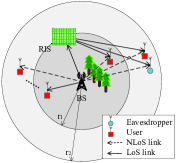
However, as shown in Fig. 2, a more general SINR expression with direct channels considered can be given as

SINRυ,RD=A2dυ,L2(𝐡^υ,σF2+𝐡^υ,RISF2).{\rm{SIN}}{{\rm{R}}_{\upsilon,{\rm{RD}}}}={A_{2}}d_{\upsilon,{\rm{L}}}^{-2}\left({\left\|{{{\widehat{\bf{h}}}_{\upsilon,\sigma}}}\right\|_{F}^{2}+\left\|{{{\widehat{\bf{h}}}_{\upsilon,{\rm{RIS}}}}}\right\|_{F}^{2}}\right). (59)

Note that deriving the exact statistical characteristics of SINRυ,RD{\rm{SIN}}{{\rm{R}}_{\upsilon,{\rm{RD}}}} are challenging, if not impossible, for calculating the performance metrics. Thus, with the help of (52) and (53), we can obtain the high-quality approximated CDF of SINRυ,RD{\rm{SIN}}{{\rm{R}}_{\upsilon,{\rm{RD}}}}.

Theorem 6.

For the second communication scenario with direct links, let Zυ,RD=SINRυ,RDZ_{\upsilon,RD}={\rm{SIN}}{{\rm{R}}_{\upsilon,RD}}, the CDF of Zυ,RDZ_{\upsilon,RD} can be expressed as

FZυ,RD(z)==12(A21zr2m(ms1)γ¯)mr2(r22r02)1GΓ(ms)Γ(m),F_{Z_{\upsilon,RD}}(z)\!=\!\prod\limits_{\ell=1}^{2}\!{{{\left(\!{\frac{{A_{2}^{-1}zr_{\hbar}^{2}{m_{{\mathcal{F}_{\ell}}}}}}{{\left({{m_{s{\mathcal{F}_{\ell}}}}-1}\right){{\bar{\gamma}}_{{\mathcal{F}_{\ell}}}}}}}\!\right)}^{{m_{{\mathcal{F}_{\ell}}}}}}\!\!\frac{{r_{\hbar}^{2}{{\left({r_{2}^{2}-r_{0}^{2}}\right)}^{-1}}G}}{{\Gamma\left({{m_{s{\mathcal{F}_{\ell}}}}}\right)\Gamma\left({{m_{{\mathcal{F}_{\ell}}}}}\right)}}}, (60)

where GG is derived as (69), shown at the top of the next page, and Gm1,n1;m2,n2;m3,n3p1,q1;p2,q2;p3,q3()G\,\!\begin{subarray}{c}m_{1},n_{1};m_{2},n_{2};m_{3},n_{3}\\ p_{1},q_{1};p_{2},q_{2};p_{3},q_{3}\end{subarray}\!(\cdot)\! denotes the Bivariate Meijer’s GG-function [55].

G=G0,2;3,2;3,20,1;1,3;1,3(=12m+1=12m,2+=12m|1m1,1ms1m1,1=12m0,=12m|1m2,1ms2m2,1=12m0,=12m|A21r2zm1(ms11)γ¯1A21r2zm2(ms21)γ¯2).\displaystyle G\!=\!G_{0,2;3,2;3,2}^{0,1;1,3;1,3}\!\!\left(\!\!\!\!{\left.{\begin{array}[]{*{20}{c}}{\sum\limits_{\ell=1}^{2}\!{{m_{{\mathcal{F}_{\ell}}}}}+1}\\ {\sum\limits_{\ell=1}^{2}\!{{m_{{\mathcal{F}_{\ell}}}}},2\!+\!\!\sum\limits_{\ell=1}^{2}\!{{m_{{\mathcal{F}_{\ell}}}}}}\end{array}}\!\!\!\right|\!\!\!\!\left.{\begin{array}[]{*{20}{c}}{1\!-\!{m_{{\mathcal{F}_{1}}}},1\!-\!{m_{s{\mathcal{F}_{1}}}}\!-\!{m_{{\mathcal{F}_{1}}}},1\!-\!\sum\limits_{\ell=1}^{2}\!{{m_{\ell}}}}\\ {0,-\sum\limits_{\ell=1}^{2}\!{{m_{{\mathcal{F}_{\ell}}}}}}\end{array}}\!\!\right|\!\!\!\!\left.{\begin{array}[]{*{20}{c}}{1\!-\!{m_{{\mathcal{F}_{2}}}},1\!-\!{m_{s{\mathcal{F}_{2}}}}\!-\!{m_{{\mathcal{F}_{2}}}},1\!-\!\sum\limits_{\ell=1}^{2}\!{{m_{{\mathcal{F}_{\ell}}}}}}\\ {0,-\sum\limits_{\ell=1}^{2}{{m_{{\mathcal{F}_{\ell}}}}}}\end{array}}\!\!\!\!\right|\!\!\!{\begin{array}[]{*{20}{c}}{\frac{{A_{2}^{-1}r_{\hbar}^{2}z{m_{{\mathcal{F}_{1}}}}}}{{\left({{m_{s{\mathcal{F}_{1}}}}-1}\right){{\bar{\gamma}}_{{\mathcal{F}_{1}}}}}}}\\ {\frac{{A_{2}^{-1}r_{\hbar}^{2}z{m_{{\mathcal{F}_{2}}}}}}{{\left({{m_{s{\mathcal{F}_{2}}}}-1}\right){{\bar{\gamma}}_{{\mathcal{F}_{2}}}}}}}\end{array}}}\!\right). (69)
Proof:

Please refer to Appendix H. ∎

Therefore, the OP of the second scenario with direct links can be expressed as OP=𝐏𝐀[FZυ,L(Zth),FZυ,RD(Zth)]T.OP={\bf{P_{A}}}{\left[{{F_{{Z_{\upsilon,L}}}}(Z_{\rm th}),{F_{{Z_{\upsilon,RD}}}}(Z_{\rm th})}\right]^{\rm T}}.

VI Numerical Results

In this section, analytical results are presented to illustrate the advantages of applying the RIS to enhance the security of the DL MIMO communication system. We assume that the noise variances σN\sigma_{N} at user nn and the eavesdropper are identical and σN=0\sigma_{N}=0 dB{\rm dB}. The transmit power pun{p_{u_{n}}} is defined in dB with respect to the noise variance. The array gains of main and sidelobes are set to Gυ=30{G_{\upsilon}}=30 dB{\rm dB} and gυ=10{g_{\upsilon}}=-10 dB{\rm dB}. For the small scale fading, we set mun=5m_{u_{n}}=5, mue=3m_{u_{e}}=3, msun=5m_{s_{u_{n}}}=5, msue=3m_{s_{u_{e}}}=3, γ¯un=γ¯ue=10{{\bar{\gamma}}_{u_{n}}}={{\bar{\gamma}}_{u_{e}}}=-10 dB{\rm dB}. The path loss exponent is set to α1=2\alpha_{1}=2. Moreover, in the considered simulation scenario, we assume that r2=400r_{2}=400, r1=300r_{1}=300, r0=1r_{0}=1, βmax=1\beta_{\rm max}=1, duR,L=30d_{u_{R},{\rm L}}=30 and B1=0.3B_{1}=0.3. The numerical results are verified via Monte-Carlo simulations by averaging the obtain performance over 10610^{6} realizations.

Refer to caption
Figure 3: Outage probability versus the transmit power for user nn.

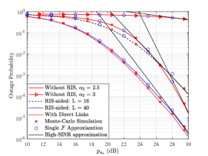
Figure 3 depicts the OP performance versus transmit power pun{p_{u_{n}}} with K=4K=4, M=2M=2, Zth=0Z_{\rm th}=0 dB{\rm dB}. As it can be observed, the OP decreases as transmit power and LL increase, which means that the introduction of a RIS can provide a higher quality of communication for the considered MIMO wireless communication system. Moreover, when α2=2.5\alpha_{2}=2.5, we can observe that RIS cannot improve the system performance when the number of reflecting elements is small. This is because the OP is dominated by the path loss. When the signal is propagates to the user via the direct links, the signal propagation distance is shorter. Furthermore, while considering the direct links exists between BS and RIS-aided users, we can observe the OP is slightly lower than while assuming no direct links exist. In addition, analytical results perfectly match the approximate ones and Monte-Carlo simulations well. In addition, the asymptotic expressions match well the exact ones at high-SINR values thus proving their validity and versatility.

Refer to caption
Figure 4: Outage probability versus the number of reflecting elements equipped in RIS.

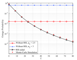
Figure 4 illustrates the OP performance versus the number of reflecting elements equipped in RIS, with K=4K=4, M=2M=2, Zth=0Z_{\rm th}=0 dB{\rm dB}, and pum=25p_{um}=25 dB{\rm dB}. In Fig. 4, we can observe that the OP decreases as LL increases. This is because the increases of RIS’s elements offer more degrees of freedom for efficient beamforming and interference management which can significantly improve the system performance. However, when the path loss of NLoS is small, applying a RIS equipped with a small number of elements, i.e., less than 25, cannot offer a lower OP than the traditional MIMO system. This is because the signal propagation distance in the direct link between the BS and user is shorter then the end-to-end link when RIS is used. In contrast, we can observe that when the path loss of NLoS is large, i.e., when α2=3\alpha_{2}=3, the performance gain brought by RIS is significant. Furthermore, when LL is sufficiently large such that the reflected signal power by the RIS dominates the total received power at user nn, we can observe that there is a diminishing return in the slope of OP due to channel hardening [56]. Thus, to achieve a low OP at the user, there exists an trade-off between the number of reflecting elements in RIS and the transmit power of the BS.

Refer to caption
Figure 5: Secrecy outage probability versus the transmit power for user nn.

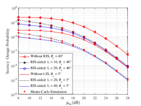
Figure 5 depicts the SOP performance versus transmit power pun{p_{u_{n}}} under different θc\theta_{c} with Rt=1R_{t}=1, K=4K=4, M=2M=2, and α2=3\alpha_{2}=3. For a certain setting of the parameters, the SOP decreases as the transmit power of the BS increases. Besides, it can be easily observed that the SOP increases as θc\theta_{c} decreases. This is because a large value of θc\theta_{c} offers the eavesdroppers a higher possibility in exploiting the larger array gains. Again, it is evident that the analytical results match the Monte-Carlo simulations well.

Refer to caption
Figure 6: Probability of non-zero secrecy capacity versus transmit power for user nn.

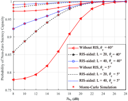
Figure 6 shows the analytical and simulated PNSC versus transmit power pun{p_{u_{n}}} under different θc\theta_{c} with Rt=1R_{t}=1, K=4K=4, M=2M=2, and α2=3\alpha_{2}=3. As it can be observed, the PNSC decreases as θc\theta_{c} increases because the eavesdropper is more likely to receive signals. Moreover, similar to the results in Fig. 5, the use of RIS can enhance the security of the system. Furthermore, if the transmit signal power is not high or the number of reflecting elements on the RIS is not large, the performance gain brought by RIS is rather then limited, as the signal propagation distance in the direct link between the BS and user is shorter then the end-to-end link when the RIS is used. However, with the increase of transmit power, the communication scenario with RIS enjoys a better security performance.

Refer to caption
Figure 7: Average security rate versus transmit power for user nn.

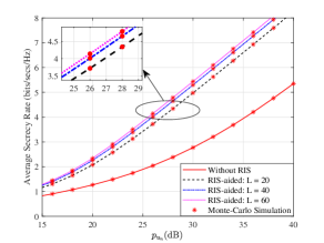
Figure 7 illustrates the ASR as a function of the transmit power pun{p_{u_{n}}} for different settings of LL with K=4K=4, M=2M=2, and α2=3\alpha_{2}=3. As expected, there is a perfect match between our analytical and simulated results. Like SOP and PNSC, when the transmit power is not large, there is only a small difference for the ASR between communication with RIS and without RIS. This is also because adopting RIS increases the signal propagation distance. In contrast, when the power is moderate to high, RIS is very useful for enhancing the security of the physical layer, and as analyzed in Remark 5, the larger the LL is, the more obvious the performance gain is. Furthermore, we can observe that there is a diminishing return in the ASR gain due to increasing LL. This is because when LL is large, the security performance of the system is mainly limited by other factors, such as the channel quality and the path loss.

VII Conclusion

We proposed a new RIS-aided secure communication system and presented the exact of expressions for CDF and PDF of the SINR for both cases of the RIS is used or not used. Our analytical framework showed the analytical performance expressions of RIS-aided communication subsume the counterpart case without exploiting RIS which can be obtained by some simple parameter transformation of the former case. Secrecy metrics, including the SOP, PNSC, and ASR, were all derived with closed-form expressions in terms of the multivariate Fox’s HH-function. Numerical results confirmed that RIS can bring significant performance gains and enhance the PLS of the considered system, especially when the number of reflecting elements is sufficiently large and the path loss of NLoS links is severe.

Appendix A Proof of Theorem 1

Based on the result derived in (18) and exploiting the fact that the elements of 𝐐υ,σ{{{\bf Q}}_{\upsilon,\sigma}} are i.n.i.d., the effective channel gain vector of user nn (eavesdropper) can be transformed into

𝐡^υ,σF2=q=1Qn=1M|qq,nυ,σ|2.\left\|{{{\widehat{\bf{h}}}_{\upsilon,\sigma}}}\right\|_{F}^{2}=\sum\limits_{q=1}^{Q}{\sum\limits_{n=1}^{M}{{{\left|{{q_{q,n}^{\upsilon,\sigma}}}\right|}^{2}}}}. (A-1)

Note that the elements of 𝐐υ,σ{{{\bf Q}}_{\upsilon,\sigma}} obey the Fisher-Snedecor \mathcal{F} distribution with fading parameters mυ,σm_{\ell}^{\upsilon,\sigma}, msυ,σm_{s_{\ell}}^{\upsilon,\sigma} and Ωυ,σ\Omega_{\ell}^{\upsilon,\sigma}. For the sake of presentation, we define {q}i=1QM={{qq,nυ,σ}n=1M}q=1Q\left\{{{q_{\ell}}}\right\}_{i=1}^{QM}=\left\{{\left\{{{q_{q,n}^{\upsilon,\sigma}}}\right\}_{n=1}^{M}}\right\}_{q=1}^{Q}.

Letting γ=γ¯|q|2/Ω\gamma_{\ell}={\bar{\gamma}_{\ell}}{{{\left|{{q_{\ell}}}\right|}^{2}}}/\Omega_{\ell}, where γ¯=𝔼[Ω]{\bar{\gamma}_{\ell}}=\mathbb{E}[\Omega_{\ell}], we have

fγ(γ)=mm((ms1)γ¯)msγm1B(m,ms)(mγ+(ms1)γ¯)m+ms.{f_{\gamma}}({\gamma_{\ell}})\!=\!\!\frac{{{m_{\ell}}^{{m_{\ell}}}\cdot{{\left({\left({{m_{{s_{\ell}}}}-1}\right){{\bar{\gamma}}_{\ell}}}\right)}^{{m_{{s_{\ell}}}}}}{\gamma_{\ell}}^{{m_{\ell}}-1}}}{{B\left({m_{\ell},{m_{s_{\ell}}}}\right){{\left({{m_{\ell}}{\gamma_{\ell}}+\left({{m_{s_{\ell}}}-1}\right){{\bar{\gamma}}_{\ell}}}\right)}^{{m_{\ell}}+{m_{{s_{\ell}}}}}}}}. (A-2)

Thus, let X==1QMγX=\sum\limits_{\ell=1}^{QM}{{\gamma_{\ell}}}, the CDF of XX is obtained with the help of [50, eq. (23)] and [49, eq (A.1)] as

FX(x)\displaystyle{F_{X}}\left(x\right) ==1QM1Γ(ms)Γ(m)12QM(12πj)QM\displaystyle=\prod\limits_{\ell=1}^{QM}{\frac{1}{{\Gamma\left({{m_{{s_{\ell}}}}}\right)\Gamma\left({{m_{\ell}}}\right)}}\int_{{{\cal L}_{1}}}{\int_{{{\cal L}_{2}}}{\cdots\int_{{{\cal L}_{{}_{QM}}}}{{{\left({\frac{1}{{2\pi j}}}\right)}^{QM}}}}}}
×1Γ(1+=1QMζ)=1QMΓ(mζ)Γ(ζ)\displaystyle\times\frac{1}{{\Gamma\left(1+{\sum\limits_{\ell=1}^{QM}{{\zeta_{\ell}}}}\right)}}\prod\limits_{\ell=1}^{QM}{\Gamma\left({{m_{\ell}}-{\zeta_{\ell}}}\right)\Gamma\left({{\zeta_{\ell}}}\right)}
×Γ(ms+ζ)(xmγ¯(ms1))ζdζ1dζQM.\displaystyle\times\Gamma\!\left({{m_{{s_{\ell}}}}\!+\!{\zeta_{\ell}}}\right)\!\!{\left(\!{\frac{{x{m_{\ell}}}}{{{{\bar{\gamma}}_{\ell}}\left({{m_{{s_{\ell}}}}-1}\right)}}}\!\right)^{{\zeta_{\ell}}}}{\rm d}{\zeta_{1}}\cdots{\rm d}{\zeta_{QM}}. (A-3)

Let D=(dum,σ)ασD=\left(d_{u_{m},\sigma}\right)^{\alpha_{\sigma}}, hence, using [32, eq. (30)], we derive the PDF of DD as

fD(d)=2(r22r02)ασd2ασ1,ifr0ασ<d<r2ασ.{f_{D}}(d)=\frac{2}{{\left({r_{2}^{2}-r_{0}^{2}}\right){\alpha_{\sigma}}}}{d^{\frac{{\rm{2}}}{{\alpha_{\sigma}}}-1}},\qquad{\rm if}\>\>\>\>{r_{0}^{\alpha_{\sigma}}<d<r_{2}^{\alpha_{\sigma}}}. (A-4)

Let us define Y=X/DY=X/D, because XX and DD are statistically independent, the CDF of YY can be formulated as

FY(y)=P{XyD}=r0ασr2ασFX(xy)fD(x)dx.{F_{Y}}\!\left(y\right)\!=\!P\left\{{X\!\leq yD}\right\}=\!\int_{r_{0}^{\alpha_{\sigma}}}^{r_{2}^{\alpha_{\sigma}}}\!\!\!\!{{F_{X}}}(xy){f_{D}}(x){\rm d}x. (A-5)

Then, by replacing (A) and (A-4) into (A-5) and exchanging the order of integration according to Fubini’s theorem, we get

FY(y)=\displaystyle{F_{Y}}\left(y\right)= 2(r22r02)ασ=1QM1Γ(mst)Γ(m)(12πj)QM\displaystyle\frac{2}{{\left({r_{2}^{2}-r_{0}^{2}}\right){\alpha_{\sigma}}}}\prod\limits_{\ell=1}^{QM}{\frac{1}{{\Gamma\left({{m_{st}}}\right)\Gamma\left({{m_{\ell}}}\right)}}{{\left({\frac{1}{{2\pi j}}}\right)}^{QM}}}
×\displaystyle\times\! 12QM1Γ(1+=1QMζ)\displaystyle\int_{{{\cal L}_{1}}}{\int_{{{\cal L}_{2}}}\cdots}\int_{{{\cal L}_{QM}}}{\frac{1}{{\Gamma\left({1+\sum\limits_{\ell=1}^{QM}{{\zeta_{\ell}}}}\right)}}}
×\displaystyle\times\! =1QMΓ(mζ)Γ(ζ)Γ(ms+ζ)(ymγ¯(ms1))ζ\displaystyle\prod\limits_{\ell=1}^{QM}\!\Gamma\!\left({{m_{\ell}}\!-{\zeta_{\ell}}}\right)\Gamma\!\left({{\zeta_{\ell}}}\right)\Gamma\left({{m_{{s_{\ell}}}}\!+\!{\zeta_{\ell}}}\right)\!{\left(\!{\frac{{y{m_{\ell}}}}{{{{\bar{\gamma}}_{\ell}}\left({{m_{{s_{\ell}}}}-1}\right)}}}\!\right)^{{\zeta_{\ell}}}}
×\displaystyle\times\! r0ασr2ασx=1QMζ+2ασ1dxIAdζ1dζ2dζQM.\displaystyle\underbrace{\int_{r_{0}^{\alpha_{\sigma}}}^{r_{2}^{\alpha_{\sigma}}}{{x^{\sum\limits_{\ell=1}^{QM}{{\zeta_{\ell}}}+\frac{2}{{\alpha_{\sigma}}}-1}}}{\rm d}x}_{{I_{A}}}{\rm d}{\zeta_{1}}{\rm d}{\zeta_{2}}\cdots{\rm d}{\zeta_{QM}}. (A-6)

IAI_{A} can easily be deduced. Letting Z=A1YZ=A_{1}Y, we obtain (22). The proof is now complete.

Appendix B Proof of Theorem 3

Based on the result derived in (20) and exploiting the fact that the elements of 𝐐3{{{\bf Q}}_{3}} and 𝐐υ,L{{{\bf Q}}_{\upsilon,{\rm L}}} are i.n.i.d., the effective channel gain vector of user nn (eavesdropper) can be transformed into

𝐡^υ,RISF2=q=1Qn=1L|(qq,nυ,L)(qn,muR,L)|2=q=1Qn=1L|qq,nυ,L|2|qn,muR,L|2.\left\|{{{\widehat{\bf{h}}}_{\upsilon,{\rm RIS}}}}\right\|_{F}^{2}\!=\!\!\!\sum\limits_{q=1}^{Q}\!{\sum\limits_{n=1}^{L}{{{\left|{\left({{q_{q,n}^{\upsilon,{\rm L}}}}\right)\left({{q_{n,m}^{u_{R},{\rm L}}}}\right)}\right|}^{2}}}}\!=\!\!\sum\limits_{q=1}^{Q}\!{\sum\limits_{n=1}^{L}{{{\left|{{q_{q,n}^{\upsilon,{\rm L}}}}\right|}^{2}}{{\left|{{q_{n,m}^{u_{R},{\rm L}}}}\right|}^{2}}}}. (B-1)

Note that qq,nυ,L(mq,nυ,L,msq,nυ,L,Ωq,nυ,L){q^{\upsilon,{\rm L}}_{q,n}}\sim{\cal F}\left({{m_{q,n}^{\upsilon,{\rm L}}}{,}{m_{{s_{q,n}}}^{\upsilon,{\rm L}}}{,}{\Omega_{q,n}^{\upsilon,{\rm L}}}}\right) and qn,muR,L(mn,muR,L,msn,muR,L,Ωn,muR,L){q_{n,m}^{u_{R},{\rm L}}}\sim{\cal F}\left({{m_{n,m}^{u_{R},{\rm L}}}{,}{m_{{s_{n,m}}}^{u_{R},{\rm L}}}{,}{\Omega_{n,m}^{u_{R},{\rm L}}}}\right) are i.n.i.d. Fisher-Snedecor \mathcal{F} RVs. Again, we define that {q}i=1QL={{(qq,nυ,L)(qn,muR,L)}n=1L}q=1Q\left\{{{q_{\ell}}}\right\}_{i=1}^{QL}=\left\{{\left\{{\left({{q_{q,n}^{\upsilon,{\rm L}}}}\right)\left({{q_{n,m}^{u_{R},{\rm L}}}}\right)}\right\}_{n=1}^{L}}\right\}_{q=1}^{Q} in order to make our proof process more concise. Thus, using [57, eq. (18)] and letting N=2N=2 and γ=γ¯|q|2Ω1,Ω2,{\gamma_{\ell}}={{\bar{\gamma}}_{\ell}}\frac{{{{\left|{{q_{\ell}}}\right|}^{2}}}}{{{\Omega_{1,\ell}}{\Omega_{2,\ell}}}}, the MGF of γ{\gamma_{\ell}} can be expressed as

Mγ(γ)=G3,22,3(m1,m2,(ms1,1)(ms2,1)γ¯γ|1,1ms1,,1ms2,m1,,m2,)Γ(m1,)Γ(ms1,)Γ(m2,)Γ(ms2,).\displaystyle{M_{\gamma}}\left({{\gamma_{\ell}}}\right)=\frac{{G_{3,2}^{2,3}\!\!\left(\!\!\!{\left.{\frac{{{m_{1,\ell}}{m_{2,\ell}}}}{{\left({{m_{{s_{1,\ell}}}}\!-\!1}\right)\!\left({{m_{{s_{2,\ell}}}}\!-\!1}\right){{\bar{\gamma}}_{\ell}}{\gamma_{\ell}}}}}\right|\!\!\!\!\begin{array}[]{*{20}{c}}{1,1\!-\!{m_{{s_{1,\ell}}}},1\!-\!{m_{{s_{2,\ell}}}}}\\ {{m_{1,\ell}},{m_{2,\ell}}}\end{array}}\!\!\!\!\right)}}{{\Gamma\left({{m_{1,\ell}}}\right)\Gamma\left({{m_{{s_{1,\ell}}}}}\right)\Gamma\left({{m_{2,\ell}}}\right)\Gamma\left({{m_{{s_{2,\ell}}}}}\right)}}. (B-4)

Letting X==1QL|γ|X=\sum\limits_{\ell=1}^{QL}{{{\left|{{\gamma_{\ell}}}\right|}}}, we can derive the PDF of XX as

fX(x)=1{X(s);x}=12πjX(s)exsds,f_{X}(x)=\mathcal{L}^{-1}\left\{\mathcal{M}_{X}(s);x\right\}=\frac{1}{2\pi j}\int_{\mathcal{L}}\mathcal{M}_{X}(s)e^{xs}{\rm d}s, (B-5)

where 1{}\mathcal{L}^{-1}\{\cdot\} denotes the inverse Laplace transform. The MGF of the XX can be expressed with the aid of (B-4) and [21, eq. (8.4.3.1)]

fX(x)\displaystyle f_{X}(x) =12πj=1QLγ(s)exsds\displaystyle=\frac{1}{{2\pi j}}\int_{\cal L}{\prod\limits_{\ell=1}^{QL}{{{\cal M}_{{\gamma_{\ell}}}}\left(s\right){e^{xs}}ds}}
=12πj=1QL(2πj)QLΓ(m1,)Γ(ms1,)Γ(m2,)Γ(ms2,)\displaystyle=\frac{1}{{2\pi j}}\int_{\cal L}{\prod\limits_{\ell=1}^{QL}{\frac{{{\left({{{2\pi j}}}\right)}^{-QL}}}{{\Gamma\left({{m_{1,\ell}}}\right)\Gamma\left({{m_{{s_{1,\ell}}}}}\right)\Gamma\left({{m_{2,\ell}}}\right)\Gamma\left({{m_{{s_{2,\ell}}}}}\right)}}}}
×QL1Υ(ζ)(m1,m2,(ms1,1)(ms2,1)γ¯s)ζ\displaystyle\times\!\!\int_{{{\cal L}_{QL}}}\!\!\!\!\!\!\!\cdots\!\!\int_{{{\cal L}_{1}}}\!\!\!\!{\Upsilon\left({{\zeta_{\ell}}}\right)}{\left({\frac{{{m_{1,\ell}}{m_{2,\ell}}}}{{\left({{m_{{s_{1,\ell}}}}\!-\!1}\right)\left({{m_{{s_{2,\ell}}}}\!-\!1}\right){{\bar{\gamma}}_{\ell}}s}}}\right)^{-{\zeta_{\ell}}}}
×exsdζ1dζQLds,\displaystyle\times{e^{xs}}{\rm d}{\zeta_{1}}\cdots{\rm d}{\zeta_{QL}}{\rm d}s, (B-6)

where

Υ(ζ)=\displaystyle\Upsilon\left({{\zeta_{\ell}}}\right)= Γ(ζ)Γ(ms1,ζ)Γ(ms2,ζ)\displaystyle\Gamma\left({-{\zeta_{\ell}}}\right)\Gamma\left({{m_{{s_{1,\ell}}}}-{\zeta_{\ell}}}\right)\Gamma\left({{m_{{s_{2,\ell}}}}-{\zeta_{\ell}}}\right)
×Γ(m1,+ζ)Γ(m2,+ζ)\displaystyle\times\Gamma\left({{m_{1,\ell}}+{\zeta_{\ell}}}\right)\Gamma\left({{m_{2,\ell}}+{\zeta_{\ell}}}\right) (B-7)

Note that the order of integration can be interchangeable according to Fubini’s theorem, we can re-write (B) as

fX(x)=\displaystyle f_{X}(x)= =1QL1Γ(m1,)Γ(ms1,)Γ(m2,)Γ(ms2,)(12πj)QL\displaystyle\prod\limits_{\ell=1}^{QL}{\frac{1}{{\Gamma\left({{m_{1,\ell}}}\right)\Gamma\left({{m_{{s_{1,\ell}}}}}\right)\Gamma\left({{m_{2,\ell}}}\right)\Gamma\left({{m_{{s_{2,\ell}}}}}\right)}}{{\left({\frac{1}{{2\pi j}}}\right)}^{QL}}}
×QL1Υ(ζ)(m1,m2,(ms1,1)(ms2,1)γ¯)ζ\displaystyle\times\!\int_{{{\cal L}_{QL}}}\!\!\!\!\!\!\cdots\!\int_{{{\cal L}_{1}}}{\Upsilon\left({{\zeta_{\ell}}}\right)}{\left(\!{\frac{{{m_{1,\ell}}{m_{2,\ell}}}}{{\left(\!{{m_{{s_{1,\ell}}}}\!-\!1}\right)\left({{m_{{s_{2,\ell}}}}-1}\right){{\bar{\gamma}}_{\ell}}}}}\!\right)^{-{\zeta_{\ell}}}}
×12πjs=1QLζexsdsIB1dζ1dζQL.\displaystyle\times\underbrace{\frac{1}{{2\pi j}}\int_{\cal L}{{s^{\sum\limits_{\ell=1}^{QL}{{\zeta_{\ell}}}}}}{e^{xs}}{\rm d}s}_{{I_{{\rm B}_{1}}}}{\rm d}{\zeta_{1}}\cdots{\rm d}{\zeta_{QL}}. (B-8)

Letting xs=txs=-t and using [21, eq. (8.315.1)], we can derive IB1I_{{{\rm B}}_{1}} as

IB1=x1=1QLζΓ1(=1QLζ).I_{{{\rm B}}_{1}}={{{x^{-1-\sum\limits_{\ell=1}^{QL}{{\zeta_{\ell}}}}}}{\Gamma^{-1}\left({-\sum\limits_{\ell=1}^{QL}{{\zeta_{\ell}}}}\right)}}. (B-9)

Substituting (B-9) into (B), we obtain the PDF of XX, which can be written as Fox’s HH function. The CDF of XX can be expressed as FX(x)=0xfr(r)𝑑r{F_{X}}\left(x\right)=\int_{0}^{x}{{f_{r}}\left(r\right)dr}. Thus, we can rewrite the CDF of XX as

FX(x)==1QL(2πj)QLΓ(m1,)Γ(ms1,)Γ(m2,)Γ(ms2,)\displaystyle{F_{X}}\left(x\right)=\prod\limits_{\ell=1}^{QL}{\frac{{{\left({{{2\pi j}}}\right)}^{-QL}}}{{\Gamma\left({{m_{1,\ell}}}\right)\Gamma\left({{m_{{s_{1,\ell}}}}}\right)\Gamma\left({{m_{2,\ell}}}\right)\Gamma\left({{m_{{s_{2,\ell}}}}}\right)}}}
×QL1Υ(ζ)Γ(=1Lζ)(m1,m2,(ms1,1)(ms2,1)γ¯)ζ\displaystyle\times\!\!\int_{{{\cal L}_{QL}}}\!\!\!\!\!\!\cdots\!\int_{{{\cal L}_{1}}}{\frac{{\Upsilon\left(\!{{\zeta_{\ell}}}\!\right)}}{{\Gamma\left({-\sum\limits_{\ell=1}^{L}{{\zeta_{\ell}}}}\right)}}}{\left({\frac{{{m_{1,\ell}}{m_{2,\ell}}}}{{\left(\!{{m_{{s_{1,\ell}}}}-1}\right)\left(\!{{m_{{s_{2,\ell}}}}-1}\!\right){{\bar{\gamma}}_{\ell}}}}}\right)^{-{\zeta_{\ell}}}}
×0xr1=1QLζdrIB2dζ1dζQL,\displaystyle\times\underbrace{\int_{0}^{x}{{r^{-1-\sum\limits_{\ell=1}^{QL}{{\zeta_{\ell}}}}}{\rm d}r}}_{{I_{{{\rm B}_{2}}}}}{\rm d}{\zeta_{1}}\cdots{\rm d}{\zeta_{QL}}, (B-10)

where IB2I_{{\rm B}_{2}} can be solved as

IB2=0xr1=1QLζdr=1=1QLζx=1QLζ.I_{{\rm B}_{2}}=\int_{0}^{x}{{r^{-1-\sum\limits_{\ell=1}^{QL}{{\zeta_{\ell}}}}}{\rm d}r}=\frac{{\rm{1}}}{{{}^{-\sum\limits_{\ell=1}^{QL}{{\zeta_{\ell}}}}}}{x^{-\sum\limits_{\ell=1}^{QL}{{\zeta_{\ell}}}}}. (B-11)

Substituting (B-11) into (B) and using [21, eq. (8.331.1)], equation (B) can be expressed as

FX(x)=\displaystyle{F_{X}}\left(x\right)= =1QL(2πj)QLΓ(m1,)Γ(ms1,)Γ(m2,)Γ(ms2,)\displaystyle\prod\limits_{\ell=1}^{QL}{\frac{{{\left({{{2\pi j}}}\right)}^{-QL}}}{{\Gamma\left({{m_{1,\ell}}}\right)\Gamma\left({{m_{{s_{1,\ell}}}}}\right)\Gamma\left({{m_{2,\ell}}}\right)\Gamma\left({{m_{{s_{2,\ell}}}}}\right)}}}
×QL1(xm1,m2,(ms1,1)(ms2,1)γ¯)ζ\displaystyle\times\int_{{{\cal L}_{QL}}}\!\!\!\!\!\!\cdots\!\!\int_{{{\cal L}_{1}}}{\left({\frac{{x{m_{1,\ell}}{m_{2,\ell}}}}{{\left({{m_{{s_{1,\ell}}}}-1}\right)\left({{m_{{s_{2,\ell}}}}-1}\right){{\bar{\gamma}}_{\ell}}}}}\right)^{-{\zeta_{\ell}}}}
×Υ(ζ)Γ(1=1Lζ)dζ1dζQL.\displaystyle\times\frac{{\Upsilon\left({{\zeta_{\ell}}}\right)}}{{\Gamma\left({1-\sum\limits_{\ell=1}^{L}{{\zeta_{\ell}}}}\right)}}{\rm d}{\zeta_{1}}\cdots{\rm d}{\zeta_{QL}}. (B-12)
Refer to caption
Figure 8: The difference between the expected distance from the user to the BS and the expected distance from the user to the RIS.

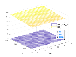
In order to avoid complex trigonometric operations, we assume that dυ,σd_{\upsilon,\sigma} and dυ,Ld_{\upsilon,{\rm L}} are i.n.i.d. RVs. To verify that this assumption will only cause small errors for our considered system, we perform Monte-Carlo simulation for the location of user nn with r0=1r_{0}=1. In the simulation, we generate the location of user nn for 10610^{6} times according to [32, eq. (30)]. Fig. 8 shows that when the distance from the RIS to the BS, defined as rRISr_{{\rm RIS}}, and the range of the system model, r2r_{2}, change, the difference between the mean distance from user nn to the BS and to the RIS is very small. For example, the maximum is less than 55 meters. Thus, let Y=X/DY=X/D, hence, we can derive the CDF of YY using (A-5)

FY(y)=2(r22r02)α=1QL(2πj)QLΓ(m1,)Γ(ms1,)Γ(m2,)Γ(ms2,)\displaystyle F_{Y}(y)\!=\!\frac{2}{{\left({r_{2}^{2}-r_{0}^{2}}\right)\alpha}}\prod\limits_{\ell=1}^{QL}{\frac{{{\left({{{2\pi j}}}\right)}^{-QL}}}{{\Gamma\left({{m_{1,\ell}}}\right)\!\Gamma\left({{m_{{s_{1,\ell}}}}}\right)\!\Gamma\left({{m_{2,\ell}}}\right)\!\Gamma\left({{m_{{s_{2,\ell}}}}}\right)}}}
×QL1Υ(ζ)Γ(1=1Lζ)(xm1,m2,(ms1,1)(ms2,1)γ¯)ζ\displaystyle\times\!\!\!\int_{{{\cal L}_{QL}}}\!\!\!\!\cdots\!\int_{{{\cal L}_{1}}}{\frac{{\Upsilon\left(\!{{\zeta_{\ell}}}\!\right)}}{{\Gamma\left({1-\sum\limits_{\ell=1}^{L}{{\zeta_{\ell}}}}\!\right)}}}{\left(\!{\frac{{x{m_{1,\ell}}{m_{2,\ell}}}}{{\left(\!{{m_{{s_{1,\ell}}}}-1}\right)\left(\!{{m_{{s_{2,\ell}}}}-1}\!\right){{\bar{\gamma}}_{\ell}}}}}\right)^{-{\zeta_{\ell}}}}
×r0αr2αy2α1=1LζdyIB3dζ1dζQL.\displaystyle\times\underbrace{\int_{{r_{0}}^{\alpha}}^{r_{2}^{\alpha}}{{y^{\frac{2}{\alpha}-1-\sum\limits_{\ell=1}^{L}{{\zeta_{\ell}}}}}}{\rm d}y}_{{I_{{{\rm B}_{3}}}}}{\rm d}{\zeta_{1}}\cdots{\rm d}{\zeta_{QL}}. (B-13)

IB3I_{{\rm B}_{3}} can be solved easily. Let α=2\alpha=2 and Z=A2YZ=A_{2}Y, we obtain (27) and complete the proof.

Appendix C Proof of Proposition 1

SOPσ,¯λSOP_{\sigma,{\mathchar 22\relax\mkern-10.0mu\lambda}} can be expressed as

SOPσ,¯λ=0FZun,σ(RsZ+Rs1)fZue,σ,¯λ(Z)dZ.SOP_{\sigma,{\mathchar 22\relax\mkern-10.0mu\lambda}}=\int_{0}^{\infty}{{F_{{Z_{{u_{n}},\sigma}}}}({R_{s}}Z+{R_{s}}-1){f_{{Z_{{u_{e}},\sigma,{\mathchar 22\relax\mkern-10.0mu\lambda}}}}}(Z)}{\rm d}Z. (C-1)

Substituting (22) and (24) into (C-1), we obtain

SOPσ,¯λ=1=1QM2=1QMΓ1(mue,s2)Γ1(mue,2)Γ(mun,s1)Γ(mun,1)\displaystyle SOP_{\sigma,{\mathchar 22\relax\mkern-10.0mu\lambda}}\!=\!\prod\limits_{{\ell_{1}}=1}^{QM}\prod\limits_{{\ell_{2}}=1}^{QM}\!\!{\frac{{{\Gamma^{-1}\left(\!{{m_{{u_{e}},{s_{{\ell_{2}}}}}}}\!\right)\!\Gamma^{-1}\left(\!{{m_{{u_{e}},{\ell_{2}}}}}\!\right)}}}{{\Gamma\left(\!{{m_{{u_{n}},{s_{{\ell_{1}}}}}}}\!\right)\!\Gamma\left(\!{{m_{{u_{n}},{\ell_{1}}}}}\!\right)}}}
×0(Hun,CDF1,2Hun,CDF1,0)(Hue,PDF1,2Hue,PDF1,0)dZ\displaystyle\!\times\!\!\!\!\int_{0}^{\infty}\!\!\!\!\!\!\!{\left(\!{{H_{{u_{n}},CD{F_{1}},2}}\!-\!{H_{{u_{n}},CD{F_{1}},0}}}\!\right)}\!\left(\!{{H_{{u_{e}},PD{F_{1}},2}}\!-\!{H_{{u_{e}},PD{F_{1}},0}}}\!\right)\!{\rm d}\!Z
𝒮2,2𝒮2,0𝒮0,2+𝒮0,0.\displaystyle\triangleq{{\cal S}_{2,2}}-{{\cal S}_{2,0}}-{{\cal S}_{0,2}}+{{\cal S}_{0,0}}. (C-2)

Substituting (28) and (30) into 𝒮p,q{{\cal S}_{p,q}} and changing the order of integration, the Integral part in 𝒮p,q{{\cal S}_{p,q}} can be expressed as

I1=0(RsZ+Rs1)1=1QMζun,1Z2=1QMζue,2dZ.I_{1}=\int_{0}^{\infty}{{{\left({{R_{s}}Z+{R_{s}}-1}\right)}^{\sum\limits_{{\ell_{1}}=1}^{QM}{{\zeta_{{u_{n}},{\ell_{1}}}}}}}{Z^{\sum\limits_{{\ell_{2}}=1}^{QM}{{\zeta_{{u_{e}},{\ell_{2}}}}}}}{\rm d}Z}. (C-3)

Let t=RsRs1Zt=\frac{{{R_{s}}}}{{{R_{s}}-1}}Z, I1I_{1} can be written as

I1=\displaystyle I_{1}= (Rs1)1=1QMζun,1(Rs1Rs)1+2=1QMζue,2\displaystyle{\left({{R_{s}}-1}\right)^{\sum\limits_{{\ell_{1}}=1}^{QM}{{\zeta_{{u_{n}},{\ell_{1}}}}}}}{\left({\frac{{{R_{s}}-1}}{{{R_{s}}}}}\right)^{{1+}\sum\limits_{{\ell_{2}}=1}^{QM}{{\zeta_{{u_{e}},{\ell_{2}}}}}}}
×0(t+1)1=1QMζun,1(t)2=1QMζue,2dtI2,\displaystyle\times\underbrace{\int_{0}^{\infty}{{{\left({t+1}\right)}^{\sum\limits_{{\ell_{1}}=1}^{QM}{{\zeta_{{u_{n}},{\ell_{1}}}}}}}{{\left(t\right)}^{\sum\limits_{{\ell_{2}}=1}^{QM}{{\zeta_{{u_{e}},{\ell_{2}}}}}}}{\rm d}t}}_{{I_{2}}}, (C-4)

let {p(t)}=P(x)\mathcal{L}\{p(t)\}=P(x). Using the property of Laplace transform, we have {0tp(z)𝑑z}=P(x)x\mathcal{L}\left\{\int_{0}^{t}p(z)dz\right\}=\frac{P(x)}{x}. According to the final value theorem, it follows that

limt(0tp(z)𝑑z)=eP(e)e=P(e).\lim_{t\rightarrow\infty}\left(\int_{0}^{t}p(z)dz\right)=e\frac{P(e)}{e}=P(e). (C-5)

Using (C-5) and [49, eq. (2.9.6)], we can solve I2I_{2} as

I2\displaystyle{I_{2}} ={(t+1)1=1QMζun,1t2=1QMζue,2}=Γ(1+2=1QMζue,2)\displaystyle\!=\!{\cal L}\left\{\!{{{\left({t+1}\right)}^{\sum\limits_{{\ell_{1}}=1}^{QM}{{\zeta_{{u_{n}},{\ell_{1}}}}}}}{{t}^{\sum\limits_{{\ell_{2}}=1}^{QM}{{\zeta_{{u_{e}},{\ell_{2}}}}}}}}\!\right\}\!=\!\Gamma\left(\!{1\!+\!\!\sum\limits_{{\ell_{2}}=1}^{QM}{{\zeta_{{u_{e}},{\ell_{2}}}}}}\!\right)
×Ψ(1+2=1QMζue,2,2+1=1QMζun,1+2=1QMζue,2,s),\displaystyle\times\Psi\left(\!{1\!+\!\!\sum\limits_{{\ell_{2}}=1}^{QM}{{\zeta_{{u_{e}},{\ell_{2}}}}},2+\!\!\!\sum\limits_{{\ell_{1}}=1}^{QM}{{\zeta_{{u_{n}},{\ell_{1}}}}}\!+\!\sum\limits_{{\ell_{2}}=1}^{QM}{{\zeta_{{u_{e}},{\ell_{2}}}}},s}\!\right), (C-6)

where Ψ()\Psi(\cdot) is the tricomi confluent hypergeometric function [21, eq. (9.210.2)]. Using [58, eq. (07.33.07.0003.01)], (C) and (C) and letting {t}=12QM+1={{ζun,1}1=1QM,{ζue,2}2=1QM,s}\left\{{{t_{\ell}}}\right\}_{\ell=1}^{2QM+1}=\left\{{\left\{{{\zeta_{{u_{n}},{\ell_{1}}}}}\right\}_{{\ell_{1}}=1}^{QM},\left\{{{\zeta_{{u_{e}},{\ell_{2}}}}}\right\}_{{\ell_{2}}=1}^{QM},s}\right\}, we can derive S2,2S_{2,2} as (46) to complete the proof.

Appendix D Proof of Proposition 2

PNSCσ,¯λPNSC_{\sigma,{\mathchar 22\relax\mkern-10.0mu\lambda}} is defined as

PNSCσ,¯λ=0FZue,σ(Z)fZun,σ(Z)dZ.PNSC_{\sigma,{\mathchar 22\relax\mkern-10.0mu\lambda}}=\int_{0}^{\infty}{{F_{{Z_{{u_{e}},\sigma}}}}}\left(Z\right){f_{{Z_{{u_{n}},\sigma}}}}\left(Z\right){\rm d}Z. (D-1)

Substituting (22) and (24) into (D-1), we obtain that

PNSCσ,¯λ=\displaystyle PNSC_{\sigma,{\mathchar 22\relax\mkern-10.0mu\lambda}}=\!\! 1=1QM1Γ(mun,s1)Γ(mun,1)2=1QM1Γ(mue,s2)Γ(mue,2)\displaystyle\prod\limits_{{\ell_{1}}=1}^{QM}\!\!{\frac{1}{{\Gamma\!\left(\!{{m_{{u_{n}},{s_{{\ell_{1}}}}}}}\!\right)\!\Gamma\left(\!{{m_{{u_{n}},{\ell_{1}}}}}\!\right)}}}\!\!\prod\limits_{{\ell_{2}}=1}^{QM}\!\!{\frac{1}{{\Gamma\!\left(\!{{m_{{u_{e}},{s_{{\ell_{2}}}}}}}\!\right)\!\Gamma\!\left(\!{{m_{{u_{e}},{\ell_{2}}}}}\!\right)}}}
×0(Hun,CDF1,2Hun,CDF1,0)\displaystyle\times\int_{0}^{\infty}{\left({{H_{{u_{n}},CD{F_{1}},2}}-{H_{{u_{n}},CD{F_{1}},0}}}\right)}
×(Hue,PDF1,2Hue,PDF1,0)dZ\displaystyle\times\left({{H_{{u_{e}},PD{F_{1}},2}}-{H_{{u_{e}},PD{F_{1}},0}}}\right){\rm d}Z
\displaystyle\triangleq 𝒫2,2𝒫2,0𝒫0,2+𝒫0,0.\displaystyle{{\cal P}_{2,2}}-{{\cal P}_{2,0}}-{{\cal P}_{0,2}}+{{\cal P}_{0,0}}. (D-2)

By changing the order of integration, we can express the integral part of 𝒫p,q{{\cal P}_{p,q}} as

I3=0Z1=1QMζun,1+2=1QMζue,2+1dZ,{I_{3}}=\int_{0}^{\infty}{{Z^{\sum\limits_{{\ell_{1}}=1}^{QM}{{\zeta_{{u_{n}},{\ell_{1}}}}}+\sum\limits_{{\ell_{2}}=1}^{QM}{{\zeta_{{u_{e}},{\ell_{2}}}}}+1}}{\rm d}Z}, (D-3)

which can be solved using the final value theorem as [53, eq. (34)]. Thus, (46) is obtained, which completes the proof.

Appendix E Proof of Proposition 3

ASCσ,λAS{C_{\sigma,\lambda}} can be expressed as

ASCσ,λ=\displaystyle AS{C_{\sigma,\lambda}}\!=\!\! i=12σ,λ,iσ,λ,3=i=12(𝒜2,2,i𝒜2,0,i𝒜0,2,i+𝒜0,0,i)\displaystyle\sum\limits_{i=1}^{2}{{{\cal I}_{\sigma,\lambda,i}}}\!-\!{{\cal I}_{\sigma,\lambda,3}}\!\!=\!\!\sum\limits_{i=1}^{2}\!{\left(\!{{{\cal A}_{2,2,i}}\!\!-\!\!{{\cal A}_{2,0,i}}\!\!-\!\!{{\cal A}_{0,2,i}}\!\!+\!\!{{\cal A}_{0,0,i}}}\!\right)}
(𝒜2,2,3𝒜2,0,3𝒜0,2,3+𝒜0,0,3),\displaystyle-\left({{{\cal A}_{2,2,3}}-{{\cal A}_{2,0,3}}-{{\cal A}_{0,2,3}}+{{\cal A}_{0,0,3}}}\right), (E-1)

where

{σ,¯λ,1=0log2(1+Z)fZun,σ(Z)FZue,σ(Z)dZ,σ,¯λ,2=0log2(1+Z)fZue,σ(Z)FZun,σ(Z)dZ,σ,¯λ,3=0log2(1+Z)fZue,σ(Z)dZ\left\{\begin{array}[]{l}\!\!\!{{\cal I}_{\sigma,\mathchar 22\relax\mkern-10.0mu\lambda,1}}\!=\!\int_{0}^{\infty}{{{\log}_{2}}}\left({1+Z}\right)\!{f_{{Z_{{u_{n}},\sigma}}}}\left(Z\right){F_{{Z_{{u_{e}},\sigma}}}}\left(Z\right){\rm d}Z,\\ \!\!\!{{\cal I}_{\sigma,\mathchar 22\relax\mkern-10.0mu\lambda,2}}\!=\!\int_{0}^{\infty}{{{\log}_{2}}}\left({1+Z}\right)\!{f_{{Z_{{u_{e}},\sigma}}}}\left(Z\right){F_{{Z_{{u_{n}},\sigma}}}}\left(Z\right){\rm d}Z,\\ \!\!\!{{\cal I}_{\sigma,\mathchar 22\relax\mkern-10.0mu\lambda,3}}\!=\!\int_{0}^{\infty}{{{\log}_{2}}}\left({1+Z}\right)\!{f_{{Z_{{u_{e}},\sigma}}}}\left(Z\right){\rm d}Z\end{array}\right. (E-2)

and

ASRσ,¯λ,i=\displaystyle ASR_{\sigma,{\mathchar 22\relax\mkern-10.0mu\lambda},i}\!=\! 1=1QM1Γ(mun,s1)Γ(mun,1)2=1QM1Γ(mue,s2)Γ(mue,2)\displaystyle\prod\limits_{{\ell_{1}}=1}^{QM}\!\!{\frac{1}{{\Gamma\!\left(\!{{m_{{u_{n}},{s_{{\ell_{1}}}}}}}\!\right)\!\Gamma\!\left(\!{{m_{{u_{n}},{\ell_{1}}}}}\!\right)}}}\!\prod\limits_{{\ell_{2}}=1}^{QM}{\frac{1}{{\!\Gamma\left(\!{{m_{{u_{e}},{s_{{\ell_{2}}}}}}}\!\right)\!\Gamma\!\left(\!{{m_{{u_{e}},{\ell_{2}}}}}\!\right)}}}
×0log2(1+Z)(Hun,CDF1,2Hun,CDF1,0)\displaystyle\times\int_{0}^{\infty}{\log_{2}}\left({1+Z}\right){\left({{H_{{u_{n}},CD{F_{1}},2}}-{H_{{u_{n}},CD{F_{1}},0}}}\right)}
×(Hue,PDF1,2Hue,PDF1,0)dZ\displaystyle\times\left({{H_{{u_{e}},PD{F_{1}},2}}-{H_{{u_{e}},PD{F_{1}},0}}}\right){\rm d}Z
\displaystyle\triangleq 𝒜2,2,i𝒜2,0,i𝒜0,2,i+𝒜0,0,i.\displaystyle{{\cal A}_{2,2,i}}-{{\cal A}_{2,0,i}}-{{\cal A}_{0,2,i}}+{{\cal A}_{0,0,i}}. (E-3)

Substituting (22) and (24) into (E-2), we can express the integral part of σ,¯λ,i{{\cal I}_{\sigma,\mathchar 22\relax\mkern-10.0mu\lambda,i}} (i=1,2)(i=1,2) as

I4=0log2(Z+1)Z1=1QMζun,1+2=1QMζue,2dZ,{I_{4}}=\int_{0}^{\infty}{{\log}_{2}\left({Z+1}\right){Z^{\sum\limits_{{\ell_{1}}=1}^{QM}{{\zeta_{{u_{n}},{\ell_{1}}}}}+\sum\limits_{{\ell_{2}}=1}^{QM}{{\zeta_{{u_{e}},{\ell_{2}}}}}}}{\rm d}Z}, (E-4)

which has been solved using the final value theorem as [53, eq. (49)]. Thus, I3{I_{3}} can be written as

I4=\displaystyle I_{4}= 1eln2SΓ(1s)Γ2(1=1QMζun,1+2=1QMζue,2)Γ(11=1QMζun,12=1QMζue,2)\displaystyle\frac{1}{{{e}\ln 2}}\int_{S}{\frac{{\Gamma\left({1-s}\right){\Gamma^{2}}\left({-\sum\limits_{{\ell_{1}}=1}^{QM}{{\zeta_{{u_{n}},{\ell_{1}}}}}+\sum\limits_{{\ell_{2}}=1}^{QM}{{\zeta_{{u_{e}},{\ell_{2}}}}}}\right)}}{{\Gamma\left({1-\sum\limits_{{\ell_{1}}=1}^{QM}{{\zeta_{{u_{n}},{\ell_{1}}}}}-\sum\limits_{{\ell_{2}}=1}^{QM}{{\zeta_{{u_{e}},{\ell_{2}}}}}}\right)}}}
×Γ(1+1=1QMζun,1+2=1QMζue,2)esds.\displaystyle\times\Gamma\left({1+\sum\limits_{{\ell_{1}}=1}^{QM}{{\zeta_{{u_{n}},{\ell_{1}}}}}+\sum\limits_{{\ell_{2}}=1}^{QM}{{\zeta_{{u_{e}},{\ell_{2}}}}}}\right){e^{s}}{\rm d}s. (E-5)

With the help of (E-2), we obtain σ,¯λ,i{{\cal I}_{\sigma,\mathchar 22\relax\mkern-10.0mu\lambda,i}} (i=1,2)(i=1,2). Similarly, following the same methodology, one can easily derive σ,¯λ,3{{\cal I}_{\sigma,\mathchar 22\relax\mkern-10.0mu\lambda,3}}. The proof is now completed.

Appendix F Proof of Theorem 5

The CDF of 1\mathcal{F}_{1} is given as [59, eq. 12]

F1(1)=m1m111m1B(m1,ms1)(ms11)m1γ¯1m1\displaystyle F_{{{\cal F}_{1}}}\left({{{\cal F}_{1}}}\right)=\frac{{{m_{{{\cal F}_{1}}}}^{{m_{{{\cal F}_{1}}}}-1}{{\cal F}_{1}}^{{m_{{{\cal F}_{1}}}}}}}{{B\left({{m_{{{\cal F}_{1}}}},{m_{s{{\cal F}_{1}}}}}\right){{\left({{m_{s{{\cal F}_{1}}}}-1}\right)}^{{m_{{{\cal F}_{1}}}}}}{{\bar{\gamma}}_{{{\cal F}_{1}}}}^{{m_{{{\cal F}_{1}}}}}}}
×F12(m1,m1+ms1,m1+1;m11(ms11)γ¯1m1).\displaystyle\times{}_{2}{F_{1}}\!\left({{m_{{{\cal F}_{1}}}},{m_{{{\cal F}_{1}}}}+{m_{s{{\cal F}_{1}}}},{m_{{{\cal F}_{1}}}}\!+1;\frac{{-{m_{{{\cal F}_{1}}}}{{\cal F}_{1}}}}{{\left({{m_{s{{\cal F}_{1}}}}-1}\right){{\bar{\gamma}}_{{{\cal F}_{1}}}}^{{m_{{{\cal F}_{1}}}}}}}}\right). (F-1)

Let us define Y=1/DY={\mathcal{F}_{1}}/D, the CDF of YY can be formulated as

FY(y)=P{1yD}=r0ασr2ασF1(1y)fD(1)d1.{F_{Y}}\left(y\right)=P\left\{{{{\cal F}_{1}}\leq yD}\right\}=\int_{r_{0}^{{\alpha_{\sigma}}}}^{r_{2}^{{\alpha_{\sigma}}}}{F_{{{\cal F}_{1}}}}({{\cal F}_{1}}y){f_{D}}({{\cal F}_{1}}){\rm{d}}{{\cal F}_{1}}. (F-2)

Substituting (F) and (A-4) into (F-2) and using [21, eq. (9.113)], we obtain

FY(y)=m1m11ym1γ¯1m1ασ(r22r02)B(m1,ms1)(ms11)m1\displaystyle{F_{Y}}\left(y\right)=\frac{{{m_{{{\cal F}_{1}}}}^{{m_{{{\cal F}_{1}}}}-1}{y^{{m_{{{\cal F}_{1}}}}}}{{\bar{\gamma}}_{{{\cal F}_{1}}}}^{-{m_{{{\cal F}_{1}}}}}}}{{{\alpha_{\sigma}}\left({r_{2}^{2}-r_{0}^{2}}\right)B\left({{m_{{{\cal F}_{1}}}},{m_{s{{\cal F}_{1}}}}}\right){{\left({{m_{s{{\cal F}_{1}}}}-1}\right)}^{{m_{{{\cal F}_{1}}}}}}}}
×Γ(m1+1)Γ(m1)Γ(m1+ms1)1πj\displaystyle\times\frac{{\Gamma\left({{m_{{{\cal F}_{1}}}}+1}\right)}}{{\Gamma\left({{m_{{{\cal F}_{1}}}}}\right)\Gamma\left({{m_{{{\cal F}_{1}}}}+{m_{s{{\cal F}_{1}}}}}\right)}}\frac{1}{{\pi j}}
×Γ(m1+t)Γ(m1+ms1+t)Γ(m1+1+t)(m1yγ¯1m1(ms11))t\displaystyle\times\int_{\cal L}{\frac{{\Gamma\left({{m_{{{\cal F}_{1}}}}+t}\right)\Gamma\left({{m_{{{\cal F}_{1}}}}+{m_{s{{\cal F}_{1}}}}+t}\right)}}{{\Gamma\left({{m_{{{\cal F}_{1}}}}+1+t}\right)}}}{\left({\frac{{{m_{{{\cal F}_{1}}}}y{{\bar{\gamma}}_{{{\cal F}_{1}}}}^{-{m_{{{\cal F}_{1}}}}}}}{{\left({{m_{s{{\cal F}_{1}}}}-1}\right)}}}\right)^{t}}
×r0ασr2ασ1t+m1+2ασ1d1IF1dt,\displaystyle\times\underbrace{\int_{r_{0}^{{\alpha_{\sigma}}}}^{r_{2}^{{\alpha_{\sigma}}}}{{\cal F}_{1}}^{t+{m_{{{\cal F}_{1}}}}+\frac{{\rm{2}}}{{{\alpha_{\sigma}}}}-1}{\rm{d}}{{\cal F}_{1}}}_{{I_{{F_{1}}}}}{\rm{d}}t, (F-3)

where the integration path of \mathcal{L} goes from tinfjt-\inf j to t+infjt+\inf j and tt\in\mathbb{R}. IF1I_{F_{1}} can be solved easily. With the help of [21, eq. (9.301)], [21, eq. (9.31.5)], [21, eq. (9.113)], [21, eq. (8.384.1)] and [21, eq. (8.331.1)], FY(y){F_{Y}}\left(y\right) can be expressed by the Meijer’s GG-function. Let Zυ,σ=A1Y{Z_{\upsilon,\sigma^{\prime}}}={A_{1}}Y, we obtain (54) that complete the proof.

Appendix G Proof of Proposition 4

With the help of [21, eq. (9.301)], eq. (55) can be expressed as (G-1), shown at the top of the next page.

G2,03,0(A1(ms11)rασm1zγ¯1m1|1,1+2ασ0,ms1,2ασ)=12πj(A1(ms11)rασm1zγ¯1m1)sΓ(s)Γ(ms1s)Γ(2ασs)Γ(1s)Γ(1+2ασs)𝑑s.G_{2,0}^{3,0}\left({\left.{\frac{A_{1}{\left({{m_{s{{\cal F}_{1}}}}-1}\right)}}{{r_{\hbar}^{{\alpha_{\sigma}}}{m_{{{\cal F}_{1}}}}z{{\bar{\gamma}}_{{{\cal F}_{1}}}}^{-{m_{{{\cal F}_{1}}}}}}}}\right|\begin{array}[]{*{20}{c}}{1,1+\frac{{\rm{2}}}{{{\alpha_{\sigma}}}}}\\ {0,{m_{s{{\cal F}_{1}}}},\frac{{\rm{2}}}{{{\alpha_{\sigma}}}}}\end{array}}\right)=\frac{1}{{2\pi j}}\int_{\cal L}{{{\left({\frac{A_{1}{\left({{m_{s{{\cal F}_{1}}}}-1}\right)}}{{r_{\hbar}^{{\alpha_{\sigma}}}{m_{{{\cal F}_{1}}}}z{{\bar{\gamma}}_{{{\cal F}_{1}}}}^{-{m_{{{\cal F}_{1}}}}}}}}\right)}^{s}}}\frac{{\Gamma\left({-s}\right)\Gamma\left({{m_{s{{\cal F}_{1}}}}-s}\right)\Gamma\left({\frac{{\rm{2}}}{{{\alpha_{\sigma}}}}-s}\right)}}{{\Gamma\left({1-s}\right)\Gamma\left({1+\frac{{\rm{2}}}{{{\alpha_{\sigma}}}}-s}\right)}}ds. (G-1)

When γ1\gamma_{\mathcal{F}_{1}}\to\infty, we have (ms11)r2ασm1zγ¯1m1{\frac{{\left({{m_{s{{\cal F}_{1}}}}-1}\right)}}{{r_{2}^{{\alpha_{\sigma}}}{m_{{{\cal F}_{1}}}}z{{\bar{\gamma}}_{{{\cal F}_{1}}}}^{-{m_{{{\cal F}_{1}}}}}}}}\to\infty. The Mellin-Barnes integral over \mathcal{L} can be calculated approximately by evaluating the residue at m-m_{\cal{F}} according to [49, Theorem 1.7]. Thus, we obtain

G2,03,0(A1(ms11)rασm1zγ¯1m1|1,1+2ασ0,ms1,2ασ)\displaystyle G_{2,0}^{3,0}\left({\left.{\frac{A_{1}{\left({{m_{s{{\cal F}_{1}}}}-1}\right)}}{{r_{\hbar}^{{\alpha_{\sigma}}}{m_{{{\cal F}_{1}}}}z{{\bar{\gamma}}_{{{\cal F}_{1}}}}^{-{m_{{{\cal F}_{1}}}}}}}}\right|\begin{array}[]{*{20}{c}}{1,1+\frac{{\rm{2}}}{{{\alpha_{\sigma}}}}}\\ {0,{m_{s{{\cal F}_{1}}}},\frac{{\rm{2}}}{{{\alpha_{\sigma}}}}}\end{array}}\right) (G-4)
γ¯1Γ(ms1+m1)m1(2ασ+m1)(r2ασm1yγ¯1m1(ms11))m1.\displaystyle\underrightarrow{{{\bar{\gamma}}_{{\mathcal{F}_{1}}}}\to\infty}\frac{{\Gamma\left({{m_{s{\mathcal{F}_{1}}}}+{m_{{\mathcal{F}_{1}}}}}\right)}}{{{m_{{\mathcal{F}_{1}}}}\left({\frac{{\text{2}}}{{{\alpha_{\sigma}}}}+{m_{{\mathcal{F}_{1}}}}}\right)}}{\left({\frac{{r_{2}^{{\alpha_{\sigma}}}{m_{{\mathcal{F}_{1}}}}y}}{{{{\bar{\gamma}}_{{\mathcal{F}_{1}}}}^{{m_{{\mathcal{F}_{1}}}}}\left({{m_{s{\mathcal{F}_{1}}}}-1}\right)}}}\right)^{{m_{{\mathcal{F}_{1}}}}}}. (G-5)

Substituting (G-4) into (54), after some algebraic manipulations, we obtain (57) and complete the proof.

Appendix H Proof of Theorem 6

With the help of (52) and (53) , the CDF of Zυ,RDZ_{\upsilon,RD} can be regarded as the CDF of sum of two Fisher \mathcal{F} RVs. Letting X=1+2X=\mathcal{F}_{1}+\mathcal{F}_{2}, using [53, eq. (12)] and [49], we can derive the CDF of XX as (H), shown at the top of the next page.

FX(x)=\displaystyle{F_{X}}\left(x\right)= =12(xm(ms1)γ¯)m(12πj)2211Γ(=12(m+s))\displaystyle{\prod\limits_{\ell=1}^{2}{\left({\frac{{x{m_{{\mathcal{F}_{\ell}}}}}}{{\left({{m_{s{\mathcal{F}_{\ell}}}}-1}\right){{\bar{\gamma}}_{{\mathcal{F}_{\ell}}}}}}}\right)}^{{m_{{\mathcal{F}_{\ell}}}}}}{\left({\frac{1}{{2\pi j}}}\right)^{2}}\int_{{\mathcal{L}_{2}}}{\int_{{\mathcal{L}_{1}}}{\frac{1}{{\Gamma\left({\sum\limits_{\ell=1}^{2}{\left({{m_{{\mathcal{F}_{\ell}}}}+{s_{\ell}}}\right)}}\right)}}}}
×=12Γ(m+s)Γ(ms+m+s)Γ(s)Γ(s+=12m)Γ(ms)Γ(m)Γ(s+=12m+1)(xm(ms1)γ¯)sds1ds2.\displaystyle\times\prod\limits_{\ell=1}^{2}{\frac{{\Gamma\left({{m_{{\mathcal{F}_{\ell}}}}+{s_{\ell}}}\right)\Gamma\left({{m_{s{\mathcal{F}_{\ell}}}}+{m_{{\mathcal{F}_{\ell}}}}+{s_{\ell}}}\right)\Gamma\left({-{s_{\ell}}}\right)\Gamma\left({{s_{\ell}}+\sum\limits_{\ell=1}^{2}{{m_{{\mathcal{F}_{\ell}}}}}}\right)}}{{\Gamma\left({{m_{s{\mathcal{F}_{\ell}}}}}\right)\Gamma\left({{m_{{\mathcal{F}_{\ell}}}}}\right)\Gamma\left({{s_{\ell}}+\sum\limits_{\ell=1}^{2}{{m_{{\mathcal{F}_{\ell}}}}}+1}\right)}}}{\left({\frac{{x{m_{{\mathcal{F}_{\ell}}}}}}{{\left({{m_{s{\mathcal{F}_{\ell}}}}-1}\right){{\bar{\gamma}}_{{\mathcal{F}_{\ell}}}}}}}\right)^{{s_{\ell}}}}d{s_{1}}d{s_{2}}. (H-1)

Let Y=X/DY=X/D, hence, we can derive the CDF of YY with the help of (A-5). Using Z=A2YZ=A_{2}Y, we can obtain the CDF of ZZ in terms of Bivariate Meijer’s GG-function as (60) to complete the proof.

References

  • [1] J. Zhang, E. Björnson, M. Matthaiou, D. W. K. Ng, H. Yang, and D. J. Love, “Prospective multiple antenna technologies for beyond 5G,” IEEE J. Sel. Areas Commun., vol. 38, no. 8, pp. 1637–1660, Aug. 2020.
  • [2] X. Yu, V. Jamali, D. Xu, D. W. K. Ng, and R. Schober, “Smart and reconfigurable wireless communications: From IRS modeling to algorithm design.” arXiv:2103.07046, 2021.
  • [3] Q. Wu and R. Zhang, “Intelligent reflecting surface enhanced wireless network via joint active and passive beamforming,” IEEE Trans. Wireless Commun., vol. 18, no. 11, pp. 5394–5409, Aug. 2019.
  • [4] C. Huang, A. Zappone, G. C. Alexandropoulos, M. Debbah, and C. Yuen, “Reconfigurable intelligent surfaces for energy efficiency in wireless communication,” IEEE Trans. Wireless Commun., vol. 18, no. 8, pp. 4157–4170, Aug. 2019.
  • [5] Q.-U.-A. Nadeem, A. Kammoun, A. Chaaban, M. Debbah, and M.-S. Alouini, “Large intelligent surface assisted MIMO communications,” arXiv:1903.08127, 2019.
  • [6] X. Chen, D. W. K. Ng, W. H. Gerstacker, and H.-H. Chen, “A survey on multiple-antenna techniques for physical layer security,” IEEE Commun. Surveys Tuts., vol. 19, no. 2, pp. 1027–1053, Feb. 2016.
  • [7] A. D. Wyner, “The wire-tap channel,” Bell Syst. Tech. J., vol. 54, no. 8, pp. 1355–1387, 1975.
  • [8] H. Du, J. Zhang, K. P. Peppas, H. Zhao, B. Ai, and X. Zhang, “On the distribution of the ratio of products of Fisher-Snedecor \mathcal{F} random variables and its applications,” IEEE Trans. Veh. Technol., vol. 69, no. 2, pp. 1855–1866, Feb. 2020.
  • [9] H.-M. Wang, T.-X. Zheng, J. Yuan, D. Towsley, and M. H. Lee, “Physical layer security in heterogeneous cellular networks,” IEEE Trans. Commun., vol. 64, no. 3, pp. 1204–1219, Mar. 2016.
  • [10] Y.-W. P. Hong, P.-C. Lan, and C.-C. J. Kuo, “Enhancing physical-layer secrecy in multiantenna wireless systems: An overview of signal processing approaches,” IEEE Signal Processing Mag., vol. 30, no. 5, pp. 29–40, May 2013.
  • [11] S. Goel and R. Negi, “Guaranteeing secrecy using artificial noise,” IEEE Trans. Wireless Commun., vol. 7, no. 6, pp. 2180–2189, Jun. 2008.
  • [12] T.-X. Zheng, H.-M. Wang, and Q. Yin, “On transmission secrecy outage of a multi-antenna system with randomly located eavesdroppers,” IEEE Commun. Lett., vol. 18, no. 8, pp. 1299–1302, Aug. 2014.
  • [13] G. Geraci, H. S. Dhillon, J. G. Andrews, J. Yuan, and I. B. Collings, “Physical layer security in downlink multi-antenna cellular networks,” IEEE Trans. Commun., vol. 62, no. 6, pp. 2006–2021, Jun. 2014.
  • [14] H.-M. Wang, C. Wang, D. W. K. Ng, M. H. Lee, and J. Xiao, “Artificial noise assisted secure transmission for distributed antenna systems,” IEEE Trans. on Signal Processing, vol. 64, no. 15, pp. 4050–4064, Apr. 2016.
  • [15] X. Zhou, R. K. Ganti, and J. G. Andrews, “Secure wireless network connectivity with multi-antenna transmission,” IEEE Trans. Wireless Commun., vol. 10, no. 2, pp. 425–430, Feb. 2010.
  • [16] X. Yu, D. Xu, and R. Schober, “Enabling secure wireless communications via intelligent reflecting surfaces,” in Proc. IEEE Global Commun. Conf., Dec. 2019, pp. 1–6.
  • [17] M. Cui, G. Zhang, and R. Zhang, “Secure wireless communication via intelligent reflecting surface,” IEEE Wireless Commun. Lett., vol. 8, no. 5, pp. 1410–1414, May 2019.
  • [18] J. Chen, Y.-C. Liang, Y. Pei, and H. Guo, “Intelligent reflecting surface: A programmable wireless environment for physical layer security,” IEEE Access, vol. 7, pp. 82 599–82 612, Jun. 2019.
  • [19] S. N. Chiu, D. Stoyan, W. S. Kendall, and J. Mecke, Stochastic geometry and its applications.   John Wiley & Sons, 2013.
  • [20] M. Haenggi, Stochastic geometry for wireless networks.   Cambridge University Press, 2012.
  • [21] I. S. Gradshteyn and I. M. Ryzhik, Table of integrals, Series, and Products, 7th ed.   Academic Press, 2007.
  • [22] X. Yu, D. Xu, Y. Sun, D. W. K. Ng, and R. Schober, “Robust and secure wireless communications via intelligent reflecting surfaces,” IEEE J. Sel. Areas Commun., vol. 38, no. 11, pp. 2637–2652, Nov. 2020.
  • [23] Z. Wang, L. Liu, and S. Cui, “Channel estimation for intelligent reflecting surface assisted multiuser communications: Framework, algorithms, and analysis,” IEEE Trans. Wireless Commun., vol. 19, no. 10, pp. 6607–6620, Oct. 2020.
  • [24] G. T. D. Araujo, A. L. F. D. Almeida, and R. Boyer, “Channel estimation for intelligent reflecting surface assisted MIMO systems: A tensor modeling approach,” IEEE J. Sel. Top. in Signal Process., pp. 1–1, 2021.
  • [25] C. Liu, X. Liu, D. W. K. Ng, and J. Yuan, “Deep residual learning for channel estimation in intelligent reflecting surface-assisted multi-user communications,” arXiv:2009.01423, 2021.
  • [26] A. Mukherjee, S. A. A. Fakoorian, J. Huang, and A. L. Swindlehurst, “Principles of physical layer security in multiuser wireless networks: A survey,” IEEE Commun. Surveys Tuts., vol. 16, no. 3, pp. 1550–1573, Mar. 2014.
  • [27] L. Yang, J. Yang, W. Xie, M. O. Hasna, T. Tsiftsis, and M. Di Renzo, “Secrecy performance analysis of RIS-aided wireless communication systems,” IEEE Trans. Veh. Technol., vol. 69, no. 10, pp. 12 296–12 300, Oct. 2020.
  • [28] M. Haenggi, J. G. Andrews, F. Baccelli, O. Dousse, and M. Franceschetti, “Stochastic geometry and random graphs for the analysis and design of wireless networks,” IEEE J. Sel. Areas Commun., vol. 27, no. 7, pp. 1029–1046, Jul. 2009.
  • [29] S. Singh, M. N. Kulkarni, A. Ghosh, and J. G. Andrews, “Tractable model for rate in self-backhauled millimeter wave cellular networks,” IEEE J. Sel. Areas Commun., vol. 33, no. 10, pp. 2196–2211, Oct. 2015.
  • [30] M. Di Renzo, “Stochastic geometry modeling and analysis of multi-tier millimeter wave cellular networks,” IEEE Trans. Wireless Commun., vol. 14, no. 9, pp. 5038–5057, Sep. 2015.
  • [31] T. Bai and R. W. Heath, “Coverage and rate analysis for millimeter-wave cellular networks,” IEEE Trans. Wireless Commun., vol. 14, no. 2, pp. 1100–1114, Feb. 2014.
  • [32] T. Hou, Y. Liu, Z. Song, X. Sun, Y. Chen, and L. Hanzo, “MIMO assisted networks relying on large intelligent surfaces: A stochastic geometry model,” arXiv:1910.00959, Feb. 2021.
  • [33] Z. Ding, F. Adachi, and H. V. Poor, “The application of MIMO to non-orthogonal multiple access,” IEEE Trans. Wireless Commun., vol. 15, no. 1, pp. 537–552, Jun. 2015.
  • [34] M. R. Akdeniz, Y. Liu, M. K. Samimi, S. Sun, S. Rangan, T. S. Rappaport, and E. Erkip, “Millimeter wave channel modeling and cellular capacity evaluation,” IEEE J. Sel. Areas Commun., vol. 32, no. 6, pp. 1164–1179, Jun. 2014.
  • [35] W. Tang, M. Z. Chen, X. Chen, J. Y. Dai, Y. Han, M. D. Renzo, Y. Zeng, S. Jin, Q. Cheng, and T. J. Cui, “Wireless communications with reconfigurable intelligent surface: Path loss modeling and experimental measurement,” IEEE Trans. Wireless Commun., vol. 20, no. 1, pp. 421–439, Jan. 2021.
  • [36] G. Nauryzbayev, K. M. Rabie, M. Abdallah, and B. Adebisi, “On the performance analysis of WPT-based dual-hop AF relaying networks in α\alpha - μ\mu fading,” IEEE Access, vol. 6, pp. 37 138–37 149, Jun. 2018.
  • [37] K. Rabie, B. Adebisi, G. Nauryzbayev, O. S. Badarneh, X. Li, and M.-S. Alouini, “Full-Duplex energy-harvesting enabled relay networks in generalized fading channels,” IEEE Wireless Commun. Lett., vol. 8, no. 2, pp. 384–387, Apr. 2019.
  • [38] S. K. Yoo, S. L. Cotton, P. C. Sofotasios, M. Matthaiou, M. Valkama, and G. K. Karagiannidis, “The Fishe-Snedecor \mathcal{F} distribution: A simple and accurate composite fading model,” IEEE Commun. Lett., vol. 21, no. 7, pp. 1661–1664, Jul. 2017.
  • [39] A. U. Makarfi, K. M. Rabie, O. Kaiwartya, O. S. Badarneh, X. Li, and R. Kharel, “Reconfigurable intelligent surface enabled IoT networks in generalized fading channels,” in Proc. IEEE ICC, 2020, pp. 1–6.
  • [40] T. J. Cui, S. Liu, and L. Zhang, “Information metamaterials and metasurfaces,” J. Mater. Chem. C, vol. 5, no. 15, pp. 3644–3668, 2017.
  • [41] D. Dardari, “Communicating with large intelligent surfaces: Fundamental limits and models,” IEEE J. Sel. Areas Commun., vol. 38, no. 11, pp. 2526–2537, Nov. 2020.
  • [42] E. Björnson and L. Sanguinetti, “Power scaling laws and Near-Field behaviors of massive MIMO and intelligent reflecting surfaces,” IEEE Open J. Commun. Soc., vol. 1, pp. 1306–1324, 2020.
  • [43] S. K. Yoo, P. C. Sofotasios, S. L. Cotton, S. Muhaidat, F. J. Lopez-Martinez, J. M. Romero-Jerez, and G. K. Karagiannidis, “A comprehensive analysis of the achievable channel capacity in \mathcal{F} composite fading channels,” IEEE Access, vol. 7, pp. 34 078 –34 094, Mar 2019.
  • [44] J. Wang, L. Kong, and M.-Y. Wu, “Capacity of wireless ad hoc networks using practical directional antennas,” in Proc. IEEE WCNC, Apr. 2010, pp. 1–6.
  • [45] Q. Wu and R. Zhang, “Beamforming optimization for wireless network aided by intelligent reflecting surface with discrete phase shifts,” IEEE Trans. Commun., vol. 68, no. 3, pp. 1838–1851, Mar. 2020.
  • [46] X. Yu, D. Xu, and R. Schober, “Optimal beamforming for MISO communications via intelligent reflecting surfaces,” in Proc. IEEE SPAWC, May 2020, pp. 1–5.
  • [47] A. M. Elbir, A. Papazafeiropoulos, P. Kourtessis, and S. Chatzinotas, “Deep channel learning for large intelligent surfaces aided mmWave massive MIMO systems,” IEEE Wireless Commun. Lett., vol. 9, no. 9, pp. 1447–1451, Sep. 2020.
  • [48] H. Du, J. Zhang, J. Cheng, Z. Lu, and B. Ai, “Millimeter wave communications with reconfigurable intelligent surfaces: Performance analysis and optimization,” IEEE Trans. Commun., to appear, 2021.
  • [49] A. M. Mathai, R. K. Saxena, and H. J. Haubold, The HH-function: Theory and Applications.   Springer Science & Business Media, 2009.
  • [50] Y. A. Rahama, M. H. Ismail, and M. S. Hassan, “On the sum of independent Fox’s HH -function variates with applications,” IEEE Trans. Veh. Technol., vol. 67, no. 8, pp. 6752–6760, Aug. 2018.
  • [51] M. Bloch, J. Barros, M. R. Rodrigues, and S. W. McLaughlin, “Wireless information-theoretic security,” IEEE Trans. Inf. Theory, vol. 54, no. 6, pp. 2515–2534, Jun. 2008.
  • [52] L. Kong and G. Kaddoum, “On physical layer security over the Fisher-Snedecor \mathcal{F} wiretap fading channels,” IEEE Access, vol. 6, pp. 39 466–39 472, Jun. 2018.
  • [53] H. Du, J. Zhang, K. P. Peppas, H. Zhao, B. Ai, and X. Zhang, “Sum of Fisher-Snedecor \mathcal{F} random variables and its applications,” IEEE Open J. Commun. Soc., vol. 1, pp. 342–356, Mar. 2020.
  • [54] Z. Zhang, C. Zhang, C. Jiang, F. Jia, J. Ge, and F. Gong, “Improving physical layer security for reconfigurable intelligent surface aided NOMA 6G networks.” arXiv:2101.06948, 2021.
  • [55] M. Shah, “On generalizations of some results and their applications,” Collectanea Mathematica, vol. 24, no. 3, pp. 249–266, 1973.
  • [56] M. Jung, W. Saad, Y. Jang, G. Kong, and S. Choi, “Performance analysis of large intelligent surfaces (LISs): Asymptotic data rate and channel hardening effects,” IEEE Trans. Wireless Commun., vol. 19, no. 3, pp. 2052–2065, Mar. 2020.
  • [57] O. S. Badarneh, S. Muhaidat, P. C. Sofotasios, S. L. Cotton, K. Rabie, and D. B. da Costa, “The N*Fisher-Snedecor \mathcal{F} cascaded fading model,” in Proc. IEEE WiMbo, Oct. 2018, pp. 1–7.
  • [58] Wolfram, “The wolfram functions site,” http://functions.wolfram.com.
  • [59] S. K. Yoo, P. C. Sofotasios, S. L. Cotton, S. Muhaidat, F. J. Lopez-Martinez, J. M. Romero-Jerez, and G. K. Karagiannidis, “A comprehensive analysis of the achievable channel capacity in \mathcal{F} composite fading channels,” IEEE Access, vol. 7, pp. 34 078–34 094, 2019.